VSLAM and Navigation System of
Unmanned Ground Vehicle
B
ased on RGB-D camera
Master of Science in Technology Thesis University of Turku
Faculty of Science and Engineering Department of Future Technologies 2018
Feng Duzhen Supervisors: Dr. Tomi Westerlund Dr. Hu Bo
The originality of this thesis has been checked in accordance with the University of Turku quality assurance system using the Turnitin Originality Check service.
FENG DUZHEN: VSLAM and Navigation System of Unmanned Ground Vehicle Based on RGB-D Camera
Master of Science in Technology Thesis, 71 p.
Digital Signal Processing and Transmission Laboratory Dec 2018
In this thesis, ROS (Robot Operating System) is used as the software platform and a simple unmanned ground vehicle that is designed and constructed by myself is used as the hardware platform. The most critical issues in the navigation technology of unmanned ground vehicles in unknown environments -SLAM (Simultaneous Localization and Mapping) and autonomous navigation technology are studied. Through the analysis of the principle and structure of visual SLAM, a visual simultaneous localization and mapping algorithm is build. Moreover, accelerate the visual SLAM algorithm through hardware replacement and software algorithm optimization. RealSense D435 is used as the camera of the VSLAM sensor. The algorithm extracts the features from the data of depth camera and calculates the odometry information of the unmanned vehicle through the features matching of the adjacent image. Then update the vehicle’s location and map data using the odometry information.
Under the condition that the visual SLAM algorithm works normally, this thesis also uses the 3D map generated to derive the real-time 2D projection map. So as to apply it to the navigation algorithm. Then this thesis realize autonomous navigation and avoids the obstacle function of unmanned vehicle by controlling the driving speed and direction of the vehicle through the navigation algorithm using the 2D projection map. Unmanned ground vehicle path planning is mainly two parts: local path planning and global path planning. Global path planning is mainly used to plan the optimal path to the destination. Local path planning is mainly used to control the speed and direction of the UGV. This thesis analyzes and compares Dijkstra’s algorithm and A* algorithm. Considering the compatible to ROS, Dijkstra’s algorithm is finally used as the global path-planning algorithm. DWA (Dynamic Window Approach) algorithm is used as Local path planning. Under the control of the Dijkstra’s algorithm and the DWA algorithm, unmanned ground vehicles can automatically plan the optimal path to the target point and avoid obstacles. This thesis also designed and constructed a simple unmanned ground vehicle as an experimental platform and design a simple control method basing on differential wheeled unmanned ground vehicle and finally realized the autonomous navigation of unmanned ground vehicles and the function of avoiding obstacles through visual SLAM algorithm and autonomous navigation algorithm.
Finally, the main work and deficiencies of this thesis are summarized. And the prospects and difficulties of the research field of unmanned ground vehicles are presented.
Keywords: Unmanned Ground Vehicle, Simultaneous Localization and Mapping, Visual SLAM, Depth camera, Navigation
Contents ... iii
Chapter One Introduction ... 1
1.1 Background ... 1
1.2 SLAM Introduction ... 2
1.3 Visual SLAM Introduction ... 4
1.4 Related Works ... 6
1.5 Outline of Thesis ... 8
Chapter Two Visual SLAM Algorithm ... 11
2.1 Depth Camera... 11
2.1.1 Time-of-Flight ... 12
2.1.2 Structured Light ... 14
2.2 RealSense Depth Camera ... 16
2.2.1 Install Librealsense... 17
2.2.2 Using RealSense Camera on ROS ... 18
2.2.3 Troubleshooting ... 19
2.3 Visual SLAM Algorithm ... 20
2.3.1 Visual Odometry ... 22
2.3.2 Loop Closure Detection ... 26
2.3.3 Back End Optimization ... 27
2.3.4 Mapping ... 28
2.4 Algorithm Optimization ... 28
2.4.1 Using RealSense D435 ... 29
2.4.2 Using Motion Graph and G2O Optimization ... 30
2.4.3 Accelerate VSLAM algorithm ... 31
Chapter Three Navigation of UGV ... 35
3.1 Configuring and Using the Navigation Stack ... 35
...
3.2.1 Global Planner ... 41
3.2.2 Local Planner ... 45
3.3 Setting Goal and Navigation ... 46
Chapter Four System Design and Implementation... 48
4.1 Vehicle Structure ... 48
4.1.1 Preparation ... 48
4.1.2 Raspberry System Installation and Car Chassis Assembly ... 49
4.1.3 Module Connection ... 49
4.1.4 Control the Car Using Raspberry PI. ... 49
4.2 Photoelectric Encoder ... 51
4.2.1 Get the Output Signal ... 51
4.2.2 Output Testing ... 52
4.3 PID Adjusting ... 52
4.3.1 Parameter Adjusting ... 55
4.3.2 Exponential Smoothing ... 57
4.3.3 Troubleshooting ... 59
4.4 System Connection and Running Unmanned Ground Vehicle ... 59
Chapter Five Conclusion and Prospect ... 65
5.1 Conclusion ... 65
5.2 Prospect ... 66
References ... 68
1
Chapter One
Introduction
1.1 Background
Since the 21st century, with the rapid economic and social development and the ever-changing science and technology, some problems in military transport, traffic safety, industrial production and cruise protection need to be solved and optimized urgently. The research of Unmanned Ground Vehicle (UGV) originated in the late 1960s [1]. With the
rapid development of artificial intelligence, machine vision, automatic control and other disciplines, Unmanned Ground Vehicle (UGV) system was born. All countries in the world are closely following the trend of science and technology. The enthusiasm for researching and developing unmanned ground vehicles is rapidly increasing, making unmanned ground vehicles technology one of the most popular research directions [2] [3].
For unmanned ground vehicles, autonomous localization and navigation in a variety of complex environments is a prerequisite for accomplishing tasks. In the process of completing the task, UGV need to realize the perception of their own location and external environment information, i.e. localization and mapping rely on various types of sensors. Only by accurately knowing the information of itself and the environment can robots accomplish tasks effectively and safely. The SLAM technology of unmanned ground vehicles has very important theoretical significance and application value. The SLAM method can improve the autonomous capabilities and environmental adaptability of unmanned ground vehicles to achieve autonomous localization and navigation in an unknown environment. It can
For unmanned ground vehicles, navigation method on SLAM does not require any trajectory to be laid in advance, which facilitates the change of navigation routes and the transformation of production lines. It can realize obstacle avoidance in real time and has strong adaptability to the environment. In the navigation control theory and research methods of ground unmanned vehicles, the navigation control methods in deterministic environments have achieved a great deal of research and application results. Some researches on the navigation control of unmanned ground vehicles in an unknown environment have also been carried out, and several methods have been proposed. However, in the visual SLAM navigation system based on the actual environment, there are still many key theoretical and technical issues that need to be solved and improved. These issues
2
include dynamic environment modeling, localization, obstacle avoidance, and path planning. Therefore, the visual SLAM and navigation technology of UGV have attracted widespread attention from scholars both in domestic and abroad.
1.2 SLAM Introduction
Assume we have made an unmanned ground vehicle; we hope it to be autonomous. We hope it can move freely in the room. It can go to the destination wherever it is. In order to make it can explore unknown environment autonomously, it need to know at least three things:
1. Where I am? --Localization.
2. What is the surrounding environment? --Mapping
3. How can I go to the destination? --Navigation
The first two things are the main mission of Simultaneously Localization and Mapping (SLAM). As an unmanned ground vehicle, on the one hand, it need to know its own status, i.e. location, on the other hand, it need to know its external environment, i.e. map. SLAM algorithms build an environment map based on the location and posture of the unmanned vehicle and determines the location and posture of the unmanned vehicle in turn from known maps. It can be described as a problem of using the sensor information to solve the problem of establishing an environmental map and determining its own position and orientation. In an unknown environment, UGV uses its own sensors to get environmental information and uses it to create and continuously update the environmental map. Based on
3
the sensor information and the created environment map, UGV can determine its own position and posture. The output of SLAM algorithm is the location of the UGV in a generated map. The map could be metrical, topological, hybrid or semantic [4]. After getting
the environment map, the UGV can driving to the destination by itself by path planning and sport controlling and then carry out its task. Fig.1.1 shows the relationship between the three things.
Of course, there are many methods to solve these two problems. For example, we can lay a guide line on the room floor, put a two-dimensional code on the wall, put radio localization equipment on the table. In the outdoors, we can also install localization devices in unmanned vehicles (like cell phones or cars). With these sensors, localization problem can be solved. We can divide these sensors into two categories. Fig.1.2 shows the different type of sensors that are used in SLAM.
One kind of sensor is installed in the environment, such as the lead rails and two-dimensional code that are already mentioned before. The sensor installed in the environment can usually directly measure the location information of the unmanned vehicle and solve the localization problem simply and effectively. However, since they must be installed in the environment, the use of unmanned vehicle is limited to some extent. For example, some places do not have GPS signals, and some places can’t lay lead rails. How to do localization?
We can see that these sensors have certain requirements on the external environment. Only when these requirements are satisfied, the localization scheme based on them can works. Or, when these requirement can’t be satisfied, we can’t localization with them.
(a) Two-dimension
(b) GPS Localization (c) Lead rails
(d) LIDAR (e) IMU
(f) Stereo camera Fig.1.2 Sensors Used in SLAM
4
Which means, although these sensors are simple and reliable, they can’t provide a universal solution of localization.
Another kind of sensor is installed on the unmanned vehicle, such as wheeled encoders, cameras, laser sensors, Inertial Measurement Unit (IMU) and so on. They measure usually indirect physical quantities rather than direct location data. For example, wheeled encoders measure the angle at which the wheel rotates, the IMU measures the angular velocity and acceleration of the motion, and the laser sensor and the camera obtain some observational data of the external environment. We can only infer our position from these data through some indirect methods. The obvious benefits are that it doesn’t place any requirement on the external environment, making this localization solution suitable for unknown environments.
In retrospect of the SLAM definition discussed earlier, we place great emphasis on the unknown environment in SLAM. In theory, we can’t limit the environment of UGV, which means we can’t assume that external sensors like GPS work well.
Therefore, the use of portable sensors to complete the SLAM is our main concern. In particular, when discussing visual SLAM (VSLAM), we mainly refer to how to solve the localization and mapping problems with camera.
1.3 Visual SLAM Introduction
According to the sensor, SLAM is mainly divided into two major categories: laser SLAM and visual SLAM. With the rapid development of computer vision, visual SLAM
has received wide attention because of its large amount of information and wide application range.
Fig.1.3 Different Type of Camera (a) Monocular camera
(b) Stereo camera
5
We will mainly talk about VSLAM in this thesis, so we are particularly concerned about what the camera can do on UGV. VSLAM camera is different with the SLR camera. Instead of carrying expensive lenses, it tends to take a picture of the surrounding environment at a rate, which will create a continuous stream of video. Ordinary camera can capture images at a rate of 30 images per second, high-speed camera is faster. According to the different working methods, the camera can be divided into monocular camera, stereo camera and depth camera that called RGB-D camera. Intuitively, the monocular camera has only one camera and stereo cameras have two or more. The principle of the RGB-D camera is more complicated. In addition to being able to get color images, it also reads out the distance between each pixel and the camera itself. Fig.1.3 shows the appearance of Cameras.
In addition, there are special or emerging type cameras such as panorama cameras, Event Cameras in VSLAM. Although they can occasionally be seen in VSLAM application, but so far have not become mainstream. The photo is essentially a projection of the scene on the imaging plane of the camera at the time the photo was taken. It reflects the three-dimensional world in two dimensions. Obviously, this process lost a dimension of the scene, which is called depth (or distance). In monocular cameras, we can’t calculate the direct distance between objects in the scene and us through a single picture. This distance is a very crucial piece of information in SLAM. Since we human beings have seen a large number of images, we have formed a natural intuition that gives us an intuitive sense of distance (space) for most scenes and helps us to determine the distances of objects in the image. For
example, we can recognize objects in an image and know the approximate size; objects in the immediate vicinity block objects in the distance; celestial objects such as the sun and the moon are generally farther away; object will be shadowed by light, and so on. This information can help us determine the object's distance, but there are also some situations
6
that may invalidate sense of distance. Fig.1.4 is an example of this situation. In this image, we can’t judge whether those small people on the palm are real people or small models only through it. Unless we change the perspective and observe the three-dimensional structure of the scene, we can get the answer. In other words, you can’t determine the true size of an object in a single image. It can be a large but distant object or it can be a close but small object. They may become the same size in the image due to their different distance.
1.4 Related Works
In China, unmanned ground vehicle is a research hotspot in universities and enterprises. The National 863 Intelligent Robot Group regards the research of intelligent mobile vehicle as the main direction for future development. The CASIA-I, a smart mobile robot developed by the Institute of Automation of the Chinese Academy of Sciences in 2003, can be widely used in hospitals, libraries, exhibition halls and other public places for services, display, homework, and personal home services. On July 14, 2011, the Hongqi HQ unmanned vehicle independently developed by the National University of Defense Technology completed the high-speed unmanned driving experiment from Changsha to Wuhan kilometers for the first time and achieved a complete success. It has created a new record of autonomous driving of autonomous ground vehicles developed by our country under complex traffic conditions, which indicates that China has made new breakthroughs in the identification of groundless environments, behavioral decision-making and control technologies. In October 2012, it was learned from the conference held by the National Natural Science Foundation of China that the self-developed unmanned ground vehicle in China will conduct a test from Beijing to Tianjin in 2014 and will test it from Beijing to Shenzhen in 2015.
The national college students' smart vehicles competition free scale cup started in 2006 and has pushed the research of unmanned vehicles to a climax. More and more colleges have invested in the research of unmanned vehicles, such as laser vehicles, infrared vehicles, and electromagnetic vehicles, camera vehicles and two-wheeled self-balancing vehicles. The number of unmanned ground vehicles that can truly achieve autonomous localization and navigation is still relatively small. In the navigation of UGV, the industry mainly focuses on autonomous patrol lines. There are UGV based on electromagnetic or laser, this navigation method is simple and stable.
7
In the past ten years after the SLAM theory was proposed, the research was mainly based on the Kalman filter algorithm framework. There are researches based on vision-based simultaneous localization and mapping algorithm of unmanned vehicles. There are also researches on vehicle localization and mapping algorithm based on laser radar ranging sensors. However, most of them are based on theoretical research. Practical applications are also limited to indoor or small-scale outdoor environments. When the vehicle is in a large-scale, irregular environment, the general SLAM algorithm is difficult to meet the requirements, which puts higher requirements on the performance and practicality of the SLAM algorithm.
Research abroad has been on mobile unmanned vehicles for many years. Their application has been infiltrated into all fields from the initial aerospace industry. In 1969, Nilsson and his colleagues at SRI (Stanford Robotics Institute) developed the first intelligent mobile robot, Shakey, equipped with rangefinders, contact sensors, and cameras, through wireless connected to the DEC.PDP 10 computer and its task is to achieve autonomous obstacle avoidance and tracking of moving targets. In the late 1970s, Hans Moravec developed the CART mobile robot at SRI. It can use cameras to avoid obstacles, and can use continuous images to construct a 2D environment model and achieve path planning.
Industrial mobile robots abroad have been used in many industries. In 2003 Kiva developed a mobile robot for logistics warehousing or large-scale automated production lines. It can move racks filled with goods back and forth between arbitrary points, put the best-selling goods to the forefront through centralized control of warehouses, and plan out the optimal path for mobile robots. Kiva's technology helps retailers speed up the execution of orders and can reduce the handling time of goods, thus greatly improving the efficiency of logistics warehousing. On July 25, 2013, KUKA Robots (Shanghai) unveiled its comprehensive and efficient automation solution at the 2013 China International Robot Exhibition (CIROS 2013). Its mobile robot platform you Bot has an omnidirectional mobile platform and a five-degrees-of-freedom arm. It also has a two-finger mechanical jaw at the end of the arm. In addition, its robotic arm and mobile platform can be used independently and can be assembled into a modern flexible production line.
Google’s autonomously-developed unmanned vehicles use sensors such as laser radar, cameras, and position estimators to observe the surrounding traffic conditions. Computers can use Lidar sensors to obtain 3-dimensional environmental maps within a 230-foot (about
8
70-meter) radius of the vehicle body. Computers can use Lidar sensors to obtain 3-dimensional environmental maps within a 230-foot (about 70-meter) radius of the vehicle body. It uses SLAM technology to provide maps for cars, allowing it to travel anywhere in the world and even find destinations for cars.
Dyson has published its 360 Heurist™ Intelligent vacuum cleaner in 2017. It use panoramic camera to run visual SLAM algorithm to get the map of the room and then plan the route of the cleaner as shown in Fig.1.5.
1.5
Outline of Thesis
This thesis mainly designed and made a VSLAM and navigation system of unmanned ground vehicle based on RGB-D camera. Firstly, the principle and framework of VSLAM algorithm and the difference between different SLAM methods are introduced. RealSense D435 is used as a sensor to implement VSLAM algorithm. Then the location and map information obtained by the VSLAM algorithm is used to achieve autonomous navigation, path planning, and obstacle avoiding of UGV. Finally, a simple UGV system is built to run the VSLAM algorithm and navigation algorithm in real environment. During the project, the NVIDIA Jetson TX2 is used as the main processor of the whole system. ROS (Robot Operating System) building on TX2 is used as a software platform to implement VSLAM and navigation algorithms. For the vehicle, Raspberry Pi and L298N dual H-bridge are used to control the wheels. The communication between TX2 and Raspberry Pi is using TCP protocol. The data from camera is sent to VSLAM algorithm to get the position and map, which will be used by the navigation algorithm. Then, the navigation algorithm will plan
9
the path of the UGV to get to the goal. It will generated the control command of UGV and send it to the raspberry pi using TCP protocol. Raspberry pi will use these commands to control L298N dual H-bridge to control the wheels.
The main structure of the system is shown as Fig.1.6. The content of the thesis is arranged as follows:
Chapter one is the introduction. It mainly describes the background, purpose and significance of the thesis and analyzes the oversea and domestic research status. Then briefly introduced the content of whole thesis.
Chapter two is visual SLAM algorithm. This chapter first introduced and analyzed the different types of visual SLAM and then briefly introduced how to use RealSense RGB-D camera and connect it to ROS. Then analyzed the general framework of visual SLAM and achieved VSLAM algorithm using RealSense RGB-D camera. Finally optimized VSLAM algorithm in both hardware and software.
Chapter three is navigation of UGV. The UGV navigation problem is modeled. Analyze and configure the conditions and data needed for navigation. Introduced several algorithms for path planning and obstacle avoiding. In addition, based on the second chapter, we achieved the navigation algorithm using Dijkstra’s and DWA algorithm.
Chapter four is system design and implementation. The whole system of this project is implemented. Introduced the construction of the car and the wheel PID adjustment control method. And add the VSLAM and navigation algorithm to the system, and use the results obtained by the navigation algorithm to control the direction and speed of the UGV. Finally show the result of running our UGV in real environment.
Chapter five is conclusion. Summarized the work and results of the entire project.
10
Pointed out the inadequacies of this project. Moreover, the prospects and difficulties of the research field of unmanned ground vehicles are presented.
11
Chapter Two
Visual SLAM Algorithm
2.1 Depth Camera
Depth cameras, also called RGB-D cameras are a kind of camera that was boom at around 2010. It is a new type of optical sensor, equipped with an optical RGB camera and depth camera. Therefore, the RGB-D camera can simultaneously obtain the optical texture information in the scene as well as the depth information of each pixel. Depth cameras generally use active imaging methods, consisting of an infrared projector and an infrared receiver. The basic structure is shown in Fig.2.1 (Kinect Generation 1 as example) [5].
Compared to monocular cameras and stereo cameras, which use the algorithm to calculate the three-dimensional coordinates of the spatial point, RGB-D cameras are more direct and convenient for acquiring 3D information of spatial points. The depth information is obtained through Structured Light or Time-of-flight(TOF) principle. It is similar to the principle of laser. Therefore, sometimes RGB-D cameras are also called Fake Lasers.
IR Projector RGB camera IR Camera
12
2.1.1 Time-of-Flight
Time-of-flight (ToF) is a relatively popular depth information acquisition method that has emerged in recent years. The time-of-flight method usually transmits a signal, and uses the time difference between signal transmission and reception to complete depth information acquisition. The time difference is different, the distance that the pulse signal walks is different, i.e. the depth information is different, it is relatively simple to operate, only need to record two times, i.e. launch time and receiving time. Fig.2.2 shows the fundamental principle of Time-of-flight [6].
The internal module of the TOF depth camera is mainly composed of a TOF area array sensor module, lighting module, control and data processing module. The lighting module is composed of infrared diode or laser diode, driving circuit, and filter circuit. It emits modulated infrared signal with infrared diode and uses a TOF area array sensor to capture the modulated signal reflected from the object. Then, the signal is converted into a digital signal by the analog-to-digital converter ADC module inside the TOF area array sensor. The converted phase data is transmitted to the control and data processing module, and the distance between the surface of the measured object and the TOF area array sensor is calculated[6][7].
According to the different modulation methods, the TOF method can generally be divided into two types: Pulsed Modulation and Continuous Wave Modulation.
13
The principle of the pulse modulation method is relatively simple, as shown in the Fig.2.3. It measures distance directly based on the time difference between pulse transmission and reception.
The measurement principle of continuous wave modulation is more complex than pulsed modulation. In practice, sine wave modulation is usually used. Since the phase shift of the sine wave at the receiving end and the transmitting end is proportional to the distance of the object from the camera, the distance can be measured by using the phase offset.
As shown in Fig.2.4, the controller in the TOF depth camera uses an infrared emitting diode to emit the modulated light signal. Blue represents the emitted light signal and red represents the reflected light signal. The area array PD sensor array receives the reflected light signal. Each pixel on the sensor array is sampled to obtain the phase difference between the emitted light and the reflected light signal to calculate the distance information. For each sampling of the TOF depth camera, four modulated light images with different receiving phases (0°, 90°, 180°, and 270°) are obtained to calculate the phase difference between the incident light and the reflected light, thereby obtaining the distance between the object and the camera [6][7][8].
Fig.2.3 Pulse Modulation Working Principle [7]
14
2.1.2 Structured Light
Structured light method is the most popular method among the active depth acquisition methods. Structured light method firstly projects the coding template actively, and at the same time use the camera to capture the deformed image after the coding template is projected into the scene [9].The unevenness of the scene is different; the deformation of the
deformed image is different from that of the coding template. The deformation variable contains the depth information we need, which is similar to the modulation and demodulation in the communication principle. When designing a coding template, a two-dimensional coding template designed usually has a certain relationship between pixels in a certain row or a certain column. Here is the pixel value information of the pixel, of course, you can also use the shape information of the pixel block, such as some encoding is a shape encoding, and some use the color information of the pixel, but the scene of the light method which using color information is usually limited in color. Otherwise, the original color in the natural scene will interfere with the color of the template itself, resulting in errors in decoding [10] [11]. Due to the fact that structured light uses specific coding information, that
is, prior information available at the time of depth calculation increases. Therefore, compared to the passive method, the structured light reduces the complexity in pixel matching [10] [11] [12].
For the structured light method, first we need a device to project an encoding template. This device is usually a digital projector. Furthermore, we need to record the deformed image that occurs after the template is projected into the scene. This device is usually a camera. With the coded template image and deformed image, we also need to deal with the correspondence between a point in the coded template image and a point in the natural scene
15
and a point in the deformed image. That is, we often say that the match, which requires the use of computers. In summary, the structural light system consisting of a camera and a projector is shown in Fig.2.5.
In recent years, the structured light method has attracted people's attention and has also had some practical applications. In the daily life of people, we can see the related products of structured light method, such as Microsoft's somatosensory game Kinect Xbox. The appearance of Microsoft's Kinect has brought profound changes to human-computer interaction. In a word, the structured light method is a promising depth information acquisition method. According to the development of the structured light method, the structured light first starts with the point structure light method, and then gradually develops into the line structure light method. Until now, the development of surface structure light method has made great progress in efficiency [12] [13].
Since depth camera is an active sensor, the quality of its three-dimensional data is almost independent of the external environment, and even in a dim environment, better quality data can be obtained due to the weakening of external light interference. Such features of RGB-D cameras make it possible to locate, map and reconstruct 3D data even in the absence of two-dimensional gray-scale features under the limited environment such as underground or in space[4][5].
16
Up to now, there are many kinds of RGB-D sensor devices on the market. More commonly used are Kinect Generation 1 and Generation 2 from Microsoft, RealSense SR300, R200, D415, D435 from Intel, Prime Sense Sensor from Prime Sense, Leap Motion from Leap and so on. Fig.2.6 shows these products.
2.2 RealSense Depth Camera
RealSense Depth camera is a RGB-D camera that composed of one color camera, two infrared receivers and one infrared emitter. Real Sense technology is Intel’s technology introduced at CES 2014 and dedicated to natural human-computer interaction. In addition to color images, it can also produce depth and infrared images information. The value of each pixel in the depth image is the distance from the camera. The depth information is derived from the binocular vision technology based on two infrared receivers and one infrared emitter. The RealSense RGB-D camera’s color camera can provides color information that can be used for reconstruction of 3D model and creating 3D color point clouds by superimposing on the depth image. In short, RealSense technology is equivalent to configuring a pair of eyes for computer equipment. The Intel Real Sense3D camera is the world's first device that integrates a 3D depth and 2D lens module and will give the device a visual depth similar to the human eye [14].
The two infrared receivers on the RealSense camera are same components and have the same settings. As shown in Fig.2.7, the imagers are marked “right” and “left” from the view of the RealSense camera module [14].
17
The depth information of RealSense RGB-D camera is get by binocular visual technology which is composed of an infrared emitter and two infrared receivers. The ASIC get the depth data from two sensors and then calculates each pixel’s depth information. Fig.2.8 shown how to reconstruct the 3D model. The following steps shows how to use RealSense RGB-D camera on Ubuntu (use RealSense R200 as example).
2.2.1 Install Librealsense
First, we should install librealsense on Ubuntu. Librealsense is a cross-platform library published by Intel. We can use it to get the raw data form RealSense RGB-D camera. This effort was initiated to better support researchers, creative coders, and app developers in domains such as robotics, virtual reality, and the internet of things.
We can download the librealsense package from GitHub. The address is
https://github.com/IntelRealSense/librealsense.
The project requires two external dependencies, glfw and libusb-1.0. The Cmake build environment additionally requires pkg-config.
To build librealsense, we should update Ubuntu distribution first. We should promote both kernel and front end. Make sure the kernel version is later than 4.4.0. Then we should install the required packages including libusb and pkg-config. After all these, we can then build the librealsense with cmake. The demos, tutorials and tests will locate in /usr/local/bin. The headers are in /usr/local/include. Moreover, the libraries are in /usr/local/lib.
Running RealSense Depth Cameras on Linux requires applying patches to kernel
18
modules. Ensure no Intel RealSense cameras are presently plugged into the system. Then install Udev rules located in librealsense source directory. Then, build the patched module for the desired machine configuration.
We can Check installation by examining the latest entries in kernel log. The log should indicate that a new uvcvideo driver has been registered. If any errors have been noted, first attempt the patching process again, and then file an issue if not successful on the second attempt (and make sure to copy the specific error in dmesg).
After installing librealsense, we can run the demos provided located in /usr/local/bin. With the demos (RealSense R200 as example), we can see the four signals images (the left image in Fig.2.8). As you can see from the picture, the position of the mouse is different. We can run another tutorial to get alignment images (the right image in Fig. 2.9).
2.2.2 Using RealSense Camera on ROS
Since ROS is the software system in this project, so we should connect RealSense RGB-D to ROS. The following steps shows how to use RealSense RGB-D camera on ROS. After we installed librealsense, we can install realsense-camera package to connect RealSense camera to ROS. We can build it from source for easy changing.
First, we can cloning sources into catkin space form https://github.com/intel-ros/realsense.git. Then build it with catkin_make. After building the realsense_camera we can run the launch file to run the RealSense file on ROS, for example: roslaunch realsense_camera r200_nodelet_default.launch
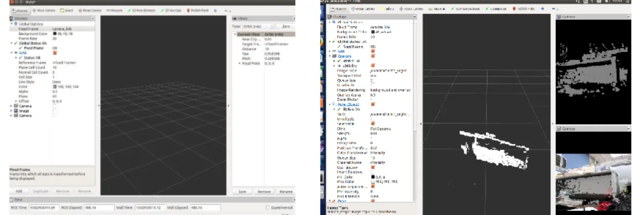
After runing the launch file, we can see the topics published by realsense_camera and the data of these topics with some command lines. Actually, there is a 3D visualization tool for ROS-rviz. We can use rviz to see the image of the camera as shown in Fig.2.10.
19
As you see from the left image, there is nothing in the rviz. If you want to see the camera image you should change the Fixed Frame to “camera_link” first. Then you can add the topic you want to show by click the “add” button on the lower-leftcornerof the window.
Also, you can just use the rviz file given in the rviz folder of realsense_camera.
2.2.3 Troubleshooting
During the installation of the librealsense, at the last step, when I run: $ make && sudo make install
There are two errors, see in Fig. 2.11:
Form the error information, we can find that it is because of the problem of the libusb. Use apt-get to re-install it.
It shows it is already the newest version. See as Fig.2.12.
Then we use Google to search this error, it shows this error is because we have install libusb before, and when we install a new version of libusb, the head file didn’t update. But
Fig. 2.10 Using Rviz
Fig.2.11 Two Errors While Installing Librealsense
20
when I try to change the head files to the newest head files, then run $ make && sudo make install. It still reports the same error. Replace doesn’t work, so I just delete the old head files. Predictably, Fig. 2.13 shows errors:
According to this information, use vim to open the file /home/zp/librealsense-master/src/uvc-v4l2.cpp
Replace the head file libusb.h with libusb-1.0/libusb.h. The Fig.2.14 shows the replaced file.
Do the same replaced on the file /home/zp/librealsense-master/src/libuvc/libuvc.h. Then run $ make && sudo make install again. Complied successfully.
2.3 Visual SLAM Algorithm
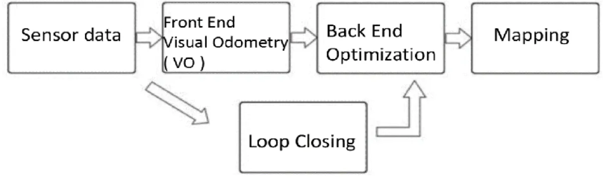
Different teams and individuals propose different VSLAM algorithms. These algorithms can be mainly divided into two parts: front-end and back-end. The front-end algorithm performs feature detection and descriptor extraction on RGB-D images, performs feature matching on the extracted descriptors, according to the matching results, the motion transformation is estimated and optimized. The back-end algorithm constructs a pose map according to the results of the front-end algorithm, then performs closed-loop detection and optimization of the pose map. Finally, the camera orientation and 3D map environment reconstruction.
Fig.2.15 VSLAM Frame
Fig. 2.13 Error after replace the head file
21
Fig.2.15 shows a classic visual SLAM frame.
The entire visual SLAM process includes the following steps:
a) Sensor data processing. It mainly is RGB-D camera image information reading and preprocessing. The sensors here include a camera, an inertial measurement unit (IMU) and so on, involving sensor selection, calibration, multi-sensor data synchronization and other technologies. It mainly is RGB-D camera image information reading and preprocessing in VSLAM.
b) Visual odometry (VO). The mission of visual odometry is to estimate the camera's motion between adjacent images, as well as the appearance of a partial map. VO is also called Front End.
c) Optimization. The back end accepts information of the camera position and attitude measured by the visual odometry at different times and the loop closure detection to optimize them, and finally get a globally consistent trajectory and map.
d) Loop closing. Loop closing detection will determine whether the robot has reached the previous position. And the information will be provided to the back end for processing and optimization.
e) Mapping. It builds a map that corresponds to the mission requirements based on the estimated trajectory.
The classic visual slam framework is the result of more than a decade of research. The framework itself and the algorithms it contains have been basically formalized and are already available in many visual and robotic program libraries. With these algorithms, we were able to build a visual slam system that allowed it to locate and map in real time under normal conditions.
22
2.3.1 Visual Odometry
The visual odometry is concerned with camera motion between adjacent images. The simplest case is of course the motion relationship between the two images. For example, when we see Fig.2.16, we will naturally reflect that the right figure should be the result of left image that rotated to left by a certain angle.
But, our intuition is not sensitive to these specific value. However, in the computer, this movement information must be accurately measured. So, how does the computer determine the motion of the camera through the image? The answer is visual odometry.
VO can estimate camera motion through the image between adjacent frames and restore the spatial structure of the scene. It is called an odometry because it is the same as the actual odometer. It only calculates the movements of the neighboring moments and is not related to the past information. At this point, VO is like a species that has only a short memory. 2.3.1.1 Feature Point
The main problem with VO is how to estimate camera motion based on the image. However, the image itself is a matrix of brightness and color, and it would be very difficult to consider the motion estimation directly from the matrix level. Therefore, we are accustomed to adopt such an approach: First, select some representative points from the image. These points will remain unchanged after a small change of camera’s perspective, so we will find same feature point in each image. Then, based on these points, the problem of camera’s posture estimation and the localization of these points can be solved. In classical SLAM frame, they are called landmarks. In the visual SLAM, the landmarks are image features. According to Wikipedia's definition, image features are a set of information related to computing tasks, and the task of computing depends on the specific application. In short, features are another digital representation of image information. A good set of features is critical to the final performance of a given task, so researchers have spent a lot
Fig.2.16 Pictures Taken by Camera and Direction of Motion [15]
23
of time investigating features. Digital images are stored in the computer as grayscale matrices, so the simplest, single image pixels are always features. However, in the visual odometer, we hope that the feature point will remain stable after the camera moves, and the gray value will be affected by the light and object material seriously. In different images, the change will be very large and unstable. Ideally, when there are small changes in the scene and the camera's perspective, we can also determine from the image which places are the same point, so the gray value alone is not enough, we need to advance the feature points on the image.
Feature points are some special places in the image. As shown in Fig.2.17, we can use the corners, edges and blocks in the image as representative areas in the image.
It is easier to point out precisely that the same corner appears in two images; the same edge is slightly more difficult, as the image is partially similar along the edge; the same block is the most difficult. We found that the corners and edges in the image are more special than those in the pixel block and their recognition between different images is stronger. Therefore, an intuitive way to extract feature points is to identify corner points between different images and confirm their correspondence. In this practice, corner points are features.
However, in most applications, the simple corners still cannot meet our needs. For this reason, researchers in the field of computer vision have designed many more stable local image features such as SIFT, ORB, etc. during their long years of research.
To extract features in an image, the first step is to calculate the "features", and then calculate the "descriptor" for the pixels surrounding those features. In OpenCV, they are calculated by cv::FeatureDetector and cv::DescriptorExtractor, respectively as shown in the
24
following program statement.
1 cv::Ptr<cv::FeatureDetector> _detector = cv::FeatureDetector::create( "ORB" );
2 cv::Ptr<cv::DescriptorExtractor> _descriptor = cv::DescriptorExtractor::create( "ORB" );
Then, use the _detector->detect() function to extract the features. It is worth
mentioning that the string can specify the type of _detector and _descriptor. If you want to build features such as FAST, SURF, just change the following string. The key point is a type of cv::KeyPoint. KeyPoint structure with Point2f pt this member variable, refers to the pixel coordinates of this feature. In addition, some features have parameters such as radius and angle, which will be drawn like a circle in the Fig.2.18.
2.3.1.2 Feature Matching
Next, we need to match the features we get from above method in adjacent images. In OpenCV, we need to choose a matching algorithm, such as bruteforce, Fast Library for Approximate Nearest Neighbour(FLANN), and so on. Here we build a FLANN matching algorithm with the following states:
1 vector< cv::DMatch > matches;
2 cv::FlannBasedMatcher matcher;
3 matcher.match( desp1, desp2, matches );
After the match is complete, the algorithm returns some DMatch structures. The structure contains the following members:
i. QueryIdx: the index of the source feature descriptor
ii. TrainIdx: the index of the target feature descriptor
25
iii. Distance: matching distance。
We can use the drawMatch function to draw the matching resulta after matching as shown in Fig.2.19:
The matching of features alone seems to be too much, it match many dissimilar features. Due to the two images only have horizontal rotation, the horizontal matching line is correct, and the others are mismatching. Therefore, you need to filter these matches, for example, to remove too large distances.
The selected goodmatch is probably like Fig.2.20.
After filtering, matching is much less, and the image looks cleaner.
After getting the match, we need to determine whether the match is successful and discard the failed data. In the previous algorithm, one result can be get for any two images. For unrelated images, it is obviously wrong. Therefore, we need to remove the matching failure. We used three methods in this project.
i. Remove frames with too few good match.
Fig.2.19 Matching of All Features [15]
26
ii. Remove frames with too few inliers in solve PnP RASNAC.
iii. Remove the case where the derived transform matrix is too large. Because the movement is coherent, the interval between two adjacent frames will not be too large.
The visual odometry is indeed the key to SLAM. However, the estimation of the trajectory through the visual odometry alone will inevitably lead to accumulating drift. This is because the visual odometer (in the simplest case) only estimates the motion between two images.
2.3.2 Loop Closure Detection
Loop closure detection mainly solves the problem of position estimation drift over time. Assume that the UGV actually returns to its origin after a period of actual movement. However, due to drift, its position estimate does not return to the original point as shown in Fig.2.21. If there is a way to let the vehicle know that it has returned to the origin, or to identify the origin, we can eliminate the drift by changing the position estimate back. This is the so-called loop closure detection.
There is a close relationship between loop closure detection and positioning and construction. In fact, we believe that the main significance of the existence of the map is to let the car know where they have been. In order to implement loop closure detection, we need to let unmanned ground vehicles have the ability to recognize the scene. There are
many ways to achieve it. In the visual SLAM, we hope that the unmanned ground vehicles can use images to accomplish this task. For example, loop closure detection can be performed by judging the similarity between images. This is similar to humans. When we
27
see two similar pictures, it is easy to recognize that they are from the same place. Therefore, visual loop closure detection is essentially an algorithm for calculating the similarity of image data. Since the information of the image is very abundant, the difficulty of correctly detecting is reduced as shown in Fig.2.22. After the loop closure is detected, we will tell the back-end optimization algorithm the information that "A and B are the same point." Then, based on this new information, the back end adjusts the trajectory and map to match the loopback detection results. In this way, if we have sufficient and correct loop closure detection, we can reduce the cumulative error and get globally consistent trajectories and maps as shown in Fig.2.23.
2.3.3 Back End Optimization
We see that the visual odometry can give a short time trajectory and map, but due to the inevitable accumulation of errors, this map is inaccurate for a long time. Therefore, based on the visual odometry, we also hope to build a larger optimization problem to consider the optimal trajectory and map over a long period of time. However, considering the balance between accuracy and performance, there are many different practices in practice.
The back end accepts information of the camera position and attitude measured by the visual odometry at different times and the loop closure detection to optimize them, and finally get a globally consistent trajectory and map. The backend accepts loopback detection information and optimizes the trajectory using graph optimization. The back end is also responsible for the noise during the SLAM process. Although we all hope that all the data are accurate, in reality, the accurate sensors also have some noise. Cheaper sensors have larger measurement errors and expensive sensors may have less error. Some sensors are
28
also affected by magnetic fields and temperature. So in addition to solving "how to estimate the camera motion from the image," we also have to care about how much noise the estimate carries, how the noise is passed from the last moment to the next moment. The problem to be considered in back-end optimization is how to estimate the state of the entire system from these noisy data, and how large the uncertainty of this state estimation is, which is called the maximum posterior probability. The state here includes both the trajectory of the vehicle itself and the map.
2.3.4 Mapping
In visual odometry, we use the feature points in the image to estimate the camera's motion. Finally, we get a rotation vector and a translation vector. Then, we can use these two vectors to stitch together the two image point clouds to form a larger point cloud.
The stitching of point clouds is essentially the process of transforming point clouds. This transformation is often described using a transform matrix:
𝑻 = [𝑹3x3 𝒕3x1 𝑶1x3 1 ] [ 𝑦1 𝑦2 𝑦3 1 ] = 𝑻 ∗ [ 𝑥1 𝑥2 𝑥3 1 ] (2-1)
The upper left portion of the matrix is a 3x3-rotation matrix, which is a quadrature array. The upper right part is a 3×1 displacement vector. The lower left is a 1×3 zoom vector, which is usually taken as 0 in SLAM because things in the environment are unlikely to suddenly become larger or smaller. The lower right corner is 1. This matrix can be transformed homogeneously on points or other things:
The process of stitch point cloud is mapping a process of building a map. The map is a description of the environment, but this description is not fixed and needs to be based on the application of SLAM.
For the unmanned ground vehicle, it mainly moves in the ground plane. Only a two-dimensional map is needed, which told UGV where it could pass, and where obstacles exist, it is enough to navigate within a certain range.
2.4 Algorithm Optimization
After all the above process, we can get a complete visual slam algorithm, but while real running the algorithm, we find it still have many problem.
29
2.4.1 Using RealSense D435
The camera that we first used is the RealSense R200, which can only get depth information within three meter due to limited power of infrared emitter. Effective depth information is not available in an environment that is too empty. When the front of the camera is relatively empty, the number of feature points extracted is insufficient only using the image and depth information on the both sides. When the car rotating, the image changes too fast, it may not be possible to get enough matched feature point pairs. Therefore, we use RealSense D435 instead. RealSense D435 camera is a new depth camera published by Intel in early 2018. It has a compact shape and is suitable for close-range depth image acquisition. It has high image resolution and sampling frame rate, and is suitable for application development of various depth information. It can get effective depth information within 10 meters, which is enough for indoor environment.
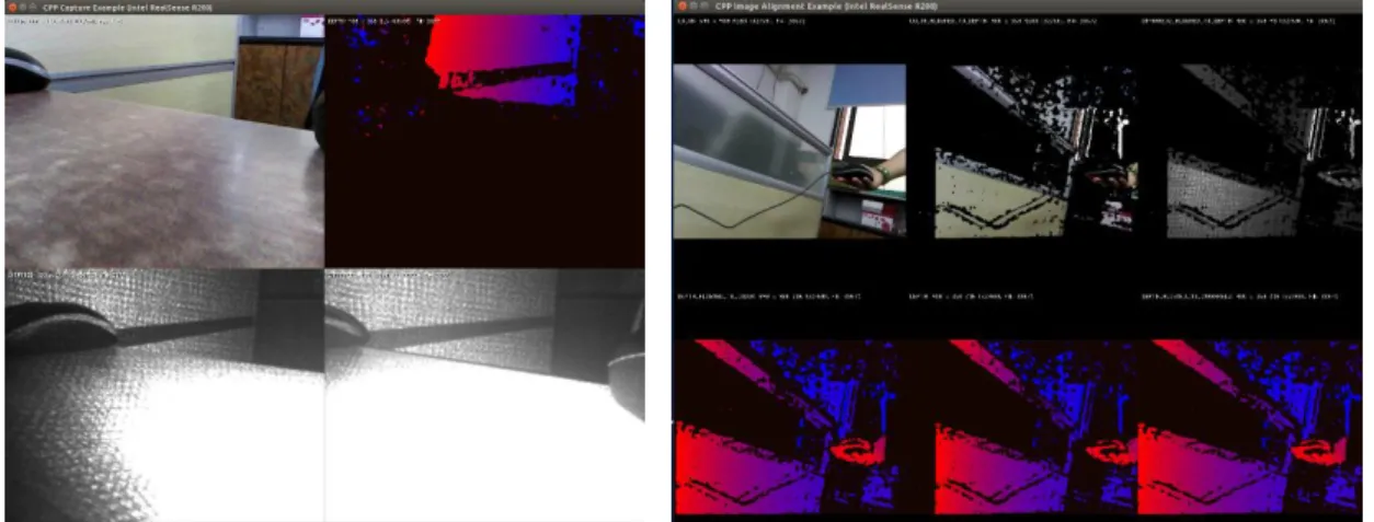
Fig.2.24 shows the data of RealSense D435, the upper left picture is the color data ,the right two pictures is the infrared data, and the lower left picture is the depth data,
30
2.4.2 Using Motion Graph and G2O Optimization
In addition, another problem is that once there is a wrong match, the entire program will crash. The deviation will always accumulate. Especially when the UGV are rotating, the sight of the camera changing very fast, it may can’t get enough feature point pairs to get accuracy motion of camera.
The cumulative deviation is unavoidable in the visual odometry. The subsequent camera’s motion is dependent on the previous motion. To ensure the accuracy of the map, we must ensure that each match is accurate which is hardly to achieve. One way is using motion graph.
The motion graph is a graph composed of camera motions. The graph here is in the sense of graph theory. A graph consists of nodes and edges G = {V, E}. In the simplest case, the nodes represent the camera's various poses, which is expressed in quaternion or matrix form:
𝒗𝑖 = [𝑥, 𝑦, 𝑧, 𝑞𝑥, 𝑞𝑦, 𝑞𝑧, 𝑞𝑤] = 𝑻𝑖 = [𝑹3x3 𝒕3x1
𝑶1x3 1 ]𝑖 (2-2) The edge refers to the transformation between the two nodes:
𝑬𝑖𝑗 = 𝑻𝑖𝑗 = [𝑹3x3 𝒕3x1
𝑶1x3 1 ]𝑖𝑗 (2-3) Then, we can put every result we previously got into a map like Fig.2.25.
Therefore, we can do VSLAM in a better way. Not only consider the information of two adjacent frames, but also consider all the information and then become a full slam problem.
Since we only compare the images of adjacent frames, it is easy to miss the match, especially when the car are turning.
Therefore, I have made an optimization. We can compare the motion changes of
31
previous multi-frame images to fix this problem. Then we will get an oriented graph as shown in Fig.2.26. The camera’s motion C3 is not only depend on motion C2 and motion
change T23 but also depend on the previous multi motion and motion changes. Then the
motion estimate become a graph optimization problem. Then we can use g2o (General Graph Optimization) to get the motion of the camera.
G2o (General Graph Optimization) is an open-source project written in C++, built with cmake. It is using for optimizing nonlinear error functions based on graph. g2o has been designed to be easily extensible to a wide range of problems and a new problem typically can be specified in a few lines of code.
The g2o core has a variety of solvers, and its vertices and edges are of various types. By customizing vertices and edges, in fact, as long as an optimization problem can be expressed as a graph, you can use g2o to solve it. Bundle adjustment, ICP, data fitting all can be done with g2o. Its GitHub address is https://github.com/RainerKuemmerle/g2o.
2.4.3 Accelerate VSLAM algorithm
Since we are comparing multi precious image for every coming image, so it need more time and computer sources. Since at the first time, we are using Intel NUC i3 as our main processor, which is may not powerful enough. Therefore, the efficiency is not satisfactory enough. Online point cloud matching is more time-consuming. So we finally use NVIDIA Jetson TX2 instead of Intel NUC I3 as VSLAM processor, using GPU to accelerate visual odometry process.
NVIDIA Jetson TX2 is an embedded system-on-module (SoM) with dual-core NVIDIA Denver2 + quad-core ARM Cortex-A57, 8GB 128-bit LPDDR4 and integrated 256-core Pascal GPU. Useful for deploying computer vision and deep learning, Jetson TX2 runs Linux and provides greater than 1TFLOPS of FP16 compute performance in less than 7.5 watts of power. NVIDIA Jetson TX2 is available as the module, developer kit, and in compatible ecosystem products.
Since NVIDIA Jetson TX2 is based on arm kernel, so it may be incompatible with librealsense the driver of RealSense camera. In order for librealsense to work properly, the kernel image must be rebuilt and patches applied to the UVC module and some other support modules. The Jetsons have the v4l2 module built into the kernel image. The module should not be built as an external module, due to needed support for the carrier board camera.
32
Because of this, a separate kernel Image should be generated, as well as any needed modules (such as the patched UVC module).
In order to support Intel RealSense cameras with built in accelerometers and gyroscopes, modules need to be enabled. These modules are in the Industrial I/O (IIO) device tree. The Jetson already has IIO support enabled in the kernel image to support the INA3321x power monitors. To support these other HID IIO devices, IIO_BUFFER must be enabled; it must be built into the kernel Image as well. Therefore, we need to do the following steps. Downloads the kernel sources for L4T from the NVIDIA website, decompresses them and opens a graphical editor on the .config file. Compiles the kernel and modules using make. The script commands make the kernel Image file, makes the module files, and installs the module files. Installing the Image file on to the system is a separate step. Note that the make is limited to the Image and modules; the rest of the kernel build (such as compiling the dts files) must be done separately.
Doing "sudo make" in the kernel source directory will build the entirety. Copies the Image file created by compiling the kernel to the /boot directory. Note that while developing you will want to be more conservative than this: You will probably want to copy the new kernel Image to a different name in the boot directory, and modify /boot/extlinux/extlinux.conf to have entry points at the old image, or the new image. This way, if things go sideways you can still boot the machine using the serial console. Removes all of the kernel sources and compressed source files. You may want to make a backup of the files before deletion.
Then after reboot TX2, we need to build librealsense 2.0 library on the TX2 to use RealSense D435. It can be described to the following steps.
Install dependencies
Applies Jetson specific patches
Sets up udev rules so the camera may be used in user space Builds librealsense, tools and demos
Installs libraries and executables
After building librealsense 2.0 library, what we need to do is to install librealsense and realsense as ROS packages, which is similar to RealSense R200. We can Cloning Intel ROS realsense package from GitHub. The address is https://github.com/intel-ros/realsense.git. Then build it under the tutorial.
33
Since we want to use the GPU on TX2 to accelerate visual odometry process, we need to rebuild OpenCV with CUDA. The version of CUDA on our TX2 is CUDA9.0, and OpenCV 3.3 incompatible with Cuda9.0. Therefore, we need to build OpenCV 3.4. After rebuilding OpenCV, we need to add OpenCV_DIR parameter to catkinConfig.cmake in our VSLAM algorithm or it will show the error: Can’t find OpencvConfig.cmake.
However, only feature point extraction supports GPU acceleration, feature point matching does not support GPU acceleration. Therefore, we still need some solution to accelerate the feature point matching algorithm.
Since TX2 is a 6-core CPU, and because of the graph optimization of the g2o, the dependency of adjacent frames is solved. Therefore, the multi-thread method can be used to simultaneously calculate the motion relationship of multiple frames and previous key frames to accelerate feature point matching as shown in Fig.2.27. For example, we can calculate the motion of C2 and C3 at the same time. We don’t need to wait until the motion
of C2 is calculated.
Moreover, there still some methods to accelerate the VSLAM algorithm. For example, since our UGV is always running in a two-dimensional ground, so we can only calculate the motion change in two dimension which only include x, y and rotation angle in this plane instead of normal SLAM motion change in three dimension.
In addition, we can use the visual odometry result of the last frame as the initial value of visual odometry of the frame. This will be useful is the speed of the UGV doesn’t change quickly.
34
Fig.2.28 shows the performance after hardware and software optimizations. As we can see from the form, while we are using Intel NUC I3, each frame need more than 300 milliseconds, we can only calculate only three frames per second. After we use NVIDIA Jetson TX2, the time consuming drop to 150ms. After we implement the software optimization, the time consuming drop to 40ms to 60ms, so we can handle 15-20 frames per second.
Fig.2.29 shows how the visual SLAM algorithm works. The upper left is the image that the camera produced. The 3D map generated by VSLAM algorithm is shown in the right. We can just move and rotate the camera by hand and we will get the 3D point cloud map. We can clearly see the wall, bookcase and books in it.
Fig.2.29 Running VSLAM Algorithm Fig.2.28 Performance Comparing
35
Chapter Three Navigation of UGV
However, since the 3D map generated by VSLAM is too big and bulky for navigation on the ground. Moreover, it is not necessary for us to use 3D map to navigate our UGV. 2D map is enough for navigation of UGV on the ground. For the point cloud getting from RGB-D camera, a simple way to get a 2RGB-D map is to convert the point cloud data into laser data, and then using some laser SLAM algorithm like gmapping to generate 2D map. But this way has waste many information provided by RGB-D camera, and it will has worse effect than a real laser. Another method is to use 3D map generated by VSLAM algorithm. We can project the 3D map onto a 2D plane, then we can use this projected map to do the navigation on the ground. In this way, not only are obstacles in one plane detected, but obstacles in a range of heights can be detected. The most problem of this method is the ground. There will be many problem if we just consider the height less than zero to be the ground since the ground may be not flat. One solution of this problem is to set a maximum angle between point's normal to ground's normal to label it as ground. Points with higher angle difference are considered as obstacles.
After fix up the 2D map, we can now run our navigation algorithm.
3.1 Configuring and Using the Navigation Stack
ROS provided a move_base package with which users can specify the position and orientation of UGV in a map that has already been established. Based on the sensor information, move_base package sends controls commands to controls the UGV to get to the target position we set. Its main features include: path planning based on odometry
36
information, outputting forward velocity and steering velocity. And you can set the maximum velocity and minimum velocity in the configuration files which will be used to make acceleration or deceleration decisions automatically. Fig.3.1 shown the content of move_base package:
The move_base package assumes that the UGV can run in a specific way. The white units are essential parts that have been done, the gray ones are optional parts, and we should implement the blue units for different UGV module. As we can see from Fig.3.1, the move_base package need a map server to provide the whole map of the environment. And it need two cost maps to preserve obstacle information in the world, which are global cost map and local cost map. Global cost map is used for path planning, creating long-term path planning throughout the environment, and local cost map is used for local path planning and obstacle avoidance.
Since we are using the map that generated by the Rtabmap algorithm in real-time, so we should change the move_base package system to the followings:
The visual odometry information is generated by Rtabmap algorithm. The map that generated by Rtabmap algorithm will be using as global map and local map. And the Rtabmap algorithm will provide a TF transform form map to odom coordinate fram which will be used to get the camera_link coordinate frame. Then we can set the goal for the UGV. And then the global planner with find a reasonablepath using global map, the local planner will get the speed of the UGV. For Differential wheel car, it including forward speed and rotation speed.
3.1.1 Transform Configuration
The move_base package need to know the real-time relationship of different coordinate
37
frames. Therefore, the UGV should publish coordinate frames information using TF.
Before configuring transform, we should firstly clear the coordinate system of the UGV. As shown in Fig.3.3. Note that the two coordinate systems are established in the right-hand coordinate system, the right hand in the left figure is the car itself, the x-axis is the forward direction, and perpendicular to the axis connection between the two wheels, the y-axis is the axis between the two wheels Connection. The figure on the right shows the car's rotational coordinate system, with the thumb pointing at the z-axis and the anticlockwise direction being positive.
Many ROS stacks need UGV platform publish a UGV transform tree based on theTFsoftware library. A TF tree set offsets between coordinate frames according to the different translation and rotation at the level of abstraction. To make it more specific, give an example of a simple UGV with a moving base on which a simple camera is installed. When referring to UGV we can set two frames: one related to moving base center and the other corresponds to the camera. We can call the frame that related to the moving base’s center "base_link". This coordinate frame is very important for navigation which will be rotational center of the UGV. And the coordinate frame corresponding to the camera can be named "camera_link".
Assuming that we get some distance data from the center point of camera. Which means, we get some distance information based on "camera_link" frame. Then we need to make the UGV platform to avoid obstacles while running use this kind of data. We should to change the distance data we’ve gotten from the "camera_link" coordinate frame to "base_link" to achieve this. Essentially, we can set a hypotaxis of the "base_link" and "camera_link" frames.
38
While setting the transform, assuming camera is installed 0.1m front and 0.2m up the moving base center. We can get a transform offset between the two frame from this information. More concretely, we can set a transform of (x: 10cm, y: 0cm, z: 20cm) to transform depth information from the "base_link" frame to the "camera_link" frame, and set the contrary transform (x: -10cm, y: 0cm, z: -20cm) to transform distance information from the "camera_link" to the "base_link".
It will be very complicated if we want to manage this relationship by ourselves when the coordinate frames increase. Fortunately, transform tree can do this work for us. We can us transform tree to define the relationship between different coordinate frames. And then, transform tree will manage the transformation between different coordinate frames automatically. If we want to use transform tree to manage the relationship between "camera_link" coordinate frame and "base_link" coordinate frames, we should add the relationship to the transform tree first, see in Fig.3.5.
In order to make sure that there is only one route between different two frames, transform tree uses a tree structure. Moreover, all slides in the tree are from parent coordinate frame to its children frames. In general, each coordinate frame should have a corresponding node in the TF tree and each transform between different frames should have a corresponding edge that is from the current coordinate frame to its child frame.
Fig.3.4 an Example of a Simple UGV
39
We can set two nodes to create a TF tree for the example we made. Each coordinate frame corresponds for one node. The relationship of the two node should be decided first to create the edge. Since all transform are from parent to child, so make sure who is parent is important. We can set "camera_link" frame to be parent node since we can get the relationship between “camera_link” coordinate frame and “map” coordinate frame from VSLAM algorithm. So the relationship of the edge between the two frames is (x: 10cm, y: 0cm, z: 20cm). We can convert the distance data that based on "camera_link" frame to "base_link", by calling the transform library after the tf setting the tf tree.
We can run “$rosrun tf view_frames” to see the TF tree in ROS.
In our UGV platform, after setting all the coordinate frame, the TF tree is shown in Fig.3.6.
40
3.1.2 Odometry Information
Since the VSLAM algorithm can get the odometry information of the UGV with VO, so we can just use it. The resulting format of VO is like the following:
1512631925.023707 0.003939 -0.006699 0.021376 0.009454 0.015106 0.001148 0.999841
The respective data are time, location (x, y, z), attitude quaternion (qx, qy, qz, qw).
Compared to Euler angles, Quaternion is a compact, easy-to-iterate method that does not exhibit singular values. Quaternion is an extended complex number that Hamilton finds. It has three imaginary parts and one real part:
𝒒 = 𝑞𝑤+ 𝑞𝑥𝑖 + 𝑞𝑦𝑗 + 𝑞𝑧𝑘 (3-1)
In which i, j, k are the three imaginary parts of the quaternion. Fig.3.7 shows the relationship of them.
Q