Durham E-Theses
An Informed Long-term Forecasting Method for
Electrical Distribution Network Operators
AKPERI, BRIAN,TEMISAN
How to cite:
AKPERI, BRIAN,TEMISAN (2017) An Informed Long-term Forecasting Method for Electrical Distribution Network Operators, Durham theses, Durham University. Available at Durham E-Theses Online:
http://etheses.dur.ac.uk/12342/
Use policy
The full-text may be used and/or reproduced, and given to third parties in any format or medium, without prior permission or charge, for personal research or study, educational, or not-for-prot purposes provided that:
• a full bibliographic reference is made to the original source
• alinkis made to the metadata record in Durham E-Theses
• the full-text is not changed in any way
The full-text must not be sold in any format or medium without the formal permission of the copyright holders.
Academic Support Oce, Durham University, University Oce, Old Elvet, Durham DH1 3HP e-mail: [email protected] Tel: +44 0191 334 6107
http://etheses.dur.ac.uk
An Informed Long-term
Forecasting Method for Electrical
Distribution Network Operators
Brian Temisan Akperi
A Thesis presented for the degree of
Doctor of Philosophy
School of Engineering and Computing Sciences
University of Durham
England
March 2017
Dedicated to
Alero Akperi and Toritse AkperiAn Informed Long-term Forecasting Method for
Electrical Distribution Network Operators
Brian Akperi
Submitted for the degree of Doctor of Philosophy
March 2017
Abstract
Northern Powergrid (NPG) is an electrical distribution network operator in the UK servicing Yorkshire and the Northeast of England. Currently they produce long-term eight year forecasts for each substation on the network with an emphasis on an annual maximum demand (MD) figure. The current method used by NPG is thought to oversimplify the problem and does not give enough insight into changes in substation demand. In order to inform their current forecast, the novel CL-ANFIS method uses a combination of machine learning techniques for both forecasting and general insight to the drivers of demand. Also introduced here are novel techniques for determination of MD at NPG and methods for handling load transfer periods.
In order to address a problem of this size, a twofold approach is taken. One is to address the drivers of demand such as weather, economic or demographic data sets through the use of statistics and machine learning techniques. The other is to address the long-term forecasting problem with a transparent technique that can aid in explaining the drivers of demand on any given substation. Techniques used include cluster analysis on demographic data sets in addition to ANFIS as a forecasting method. The results of the novel CL-ANFIS method are compared against the current NPG forecast and show how more insight into substation demand profiles can drive the decision-making process. This is done through a combination of using a tailored customer database for NPG and leveraging the information provided by the membership functions of ANFIS.
Publications
Conference Papers
1. B. Akperi and P. Matthews. Analysis of Clustering Techniques on Load
Profiles for Electrical Distribution. 2014 IEEE International Conference on Power System Technology (POWERCON), 2014a.
2. B. Akperi and P. Matthews. Analysis of Customer Profiles on an Electrical
Distribution Network. 2014 49th International Universities Power Engineering Conference (UPEC), 2014b.
Declaration
The work in this thesis is based on research carried out at Durham University, the School of Engineering and Computing Sciences, England. No part of this thesis has been submitted elsewhere for any other degree or qualification and it is all my own work unless referenced to the contrary in the text.
Copyright c 2017 by Brian Temisan Akperi.
“The copyright of this thesis rests with the author. No quotations from it should be published without the author’s prior written consent and information derived from it should be acknowledged”.
Acknowledgements
I would like to thank the following people who have helped me achieve the results presented in this thesis:
• My supervisor Dr. Peter Matthews for allowing me to work on an interesting project and providing his support and guidance.
• The sponsor Northern Powergrid for putting forth this interesting research project and in particular Alan Creighton and Suninder Deagon for their help.
• Dr. Douglas Halliday and all the members of the multidisciplinary CDT in energy.
• My good friend Guanmei (Mona) Wang who gave me the crazy idea of doing a PhD in the first place.
• Riccardo Iacopetta Shirres for doing some good work in implementing methods presented here for NPG use.
• The support of my mother Eveline Pellenkoft and father Mejuya Akperi whom I love dearly.
• Alero and Toritse for giving me the motivation to carry on.
Acronyms
ACF Auto Correlation Function
ACS Average Cold Spell Correction
ANFIS Adaptive Neuro-based approach to Fuzzy Inference Systems
ANN Artificial Neural Network
ARIMA Autoregressive Integrated Moving Average
ARMA Autoregressive Moving Average
BEIS Department for Business, Energy and Industrial Strategy
BIS Department for Business, Innovation and Skills
CHP Combined Heat and Power
CL-ANFIS Customer-Led ANFIS
CLNR Customer-Led Network Revolution
CRI Composite Risk Index
DECC Department of Energy and Climate Change
DLE Distribution Load Estimate
DNO Distribution Network Operator
DT Decision Tree
EHV Extra High Voltage
EMU European Monetary Union
FIS Fuzzy Inference System
GA Genetic Algorithm
Acronyms viii
GENEFER Genetic Neural Fuzzy Explorer
GSP Grid Supply Point
HW Holt Winters exponential smoothing
KNN K Nearest Neighbour
LSE Least Squares Estimate
LV Low Voltage
MAE Mean Absolute Error
MAP Maximum a Posteriori estimation
MAPE Mean Absolute Percentage Error
MD Maximum Demand
MIDAS Met Office Integrated Data Archive System
MSE Mean Squared Error
NB Na¨ıve Bayes
NEM National Electricity Market (of Australia)
NG National Grid
NPG Northern Powergrid
OAC Output Area Classification
Ofgem Office of Gas and Electricity Markets
ONS Office of National Statistics
PCA Principal Component Analysis
PDF Probability Density Function
RBFNN Radial Basis Function Neural Network
RIPPER Repated Incremental Pruning to Produce Error Reduction
RMS Root Mean Square
RMSE Root Mean Squared Error
RQ Research Question
Acronyms ix SVM Support Vector Machine
TAIEX Taiwan Capitalization Weighted Stock Index
TPC Taiwan Power Company
Nomenclature
ACC Accuracy
AR(p) Autoregressive model of orderp
C Matrix of cluster centres for fuzzy C-means (Section 3.2.7)
CVk K-fold cross validation error
F N False Negative
F P False Positive
F P R False Positive Rate
Ft Holt Winters time series (Section 6.2.3)
H0 Null hypothesis
I Current
I(·) Indicator function
K Number of K closest neighbours (Section 3.2.2)
K Number of K clusters (Section 3.2.6)
M Non-adjusted MD (Section 2.3.2)
M A(q) Moving average model of order q M CC Matthew’s Correlation Coefficient
Macs ACS MD (Section 2.3.2)
O1
A,i Membership function for a fuzzy setAi
P Real Power
P(·) Probability of event
Q Reactive Power
RSS(·,·) Residual sum of squares
R2 Coefficient of determination x
Nomenclature xi
S Apparent Power
S Xie-Beni index (Section 6.2.1)
S(A, B) Similarity measure between fuzzy sets A and B (Section 6.2.2)
T Output layer terms (Section 3.2.7)
T Dunn index (Section 6.2.1)
T N True Negative
T P True Positive
T P R True Positive Rate
T−1 Noon temperature on day before MD day (Section 2.3.2)
T−2 Noon temperature two days before MD day (Section 2.3.2)
T0 Noon temperature on day of MD (Section 2.3.2)
Tc Effective Temperature (Section 2.3.2)
V Voltage
Vj) Function space
X Input layer terms (Section 3.2.7)
Z Hidden layer terms (Section 3.2.7) ¯
R Davies-Bouldin index (Section 4.3.1)
χ2 Chi-squared test of independence
γ(·,·) Covariance of two time series (Section 3.2.7)
µ Mean of distribution
µAi(x) Membership function for a fuzzy setAi
φ Haar father wavelet
ψ Haar mother wavelet
ρ(·,·) Autocorrelation function
σ Standard deviation
σ(x) Sigmoid function
errtrain Training error
var(·) Variance
a Width of generalised bell membership function (Section 6.6)
Nomenclature xii
bt Holt Winters linear trend component
c Centre of generalised bell membership function (Section 6.6)
ct Holt Winters seasonal correction factor
d(·,·) Distance metric
fi Forecasted MD values
k Kurtosis value (Section 5.1.1)
n Sample size
p p value (Section 4.1)
pi Probability for event i
s(i) Silhouette value (Section 7.1)
s.e. Standard error
st Holt Winters base signal (Section 6.2.3)
t t score (Section 4.1)
Contents
Abstract iii Declaration v Acknowledgements vi Acronyms vii Nomenclature x 1 Introduction 11.1 Challenges Facing Northern Powergrid . . . 1
1.1.1 Uncertainties With the Raw SCADA Data . . . 2
1.1.2 Uncertainty in Interpreting the Raw Data . . . 2
1.1.3 Future Uncertainties . . . 3
1.2 Current Challenges in Long-Term Demand Forecasting . . . 4
1.3 Research Questions . . . 8
1.4 Research Contributions . . . 9
1.5 Structure of Thesis . . . 10
2 The Current Northern Powergrid Method 12 2.1 The Role of Northern Powergrid in Electricity Distribution . . . 12
2.1.1 Definitions and Basic Overview of Northern Powergrid Method 14 2.2 Load Related Drivers . . . 15
2.3 Northern Powergrid Methodology . . . 16
2.3.1 Determination of Maximum Demand . . . 17 xiii
Contents xiv
2.3.2 Average Cold Spell Correction . . . 19
2.3.3 Load Forecasting for Underlying Growth . . . 21
2.3.4 Forecasting Large Load Changes . . . 24
2.3.5 Distribution Load Estimate and Firm Capacity . . . 25
2.3.6 Overall Load Estimate Process Problems . . . 26
2.4 Conclusion . . . 27
3 Techniques for Load Analysis 28 3.1 General Techniques in Machine Learning . . . 28
3.1.1 Supervised Learning . . . 28
3.1.2 Unsupervised Learning . . . 33
3.1.3 Methods for Time Series and Forecasting . . . 38
3.1.4 Conclusion on General Techniques in Machine Learning . . . . 44
3.2 Industry Case Studies . . . 44
3.2.1 Finance . . . 44
3.2.2 Weather . . . 47
3.2.3 Electrical Distribution . . . 49
3.3 Conclusion . . . 54
3.3.1 Supporting the Need for New Research . . . 55
4 Data Mining for Informed Substation Trends 57 4.1 Temperature and Weather Considerations . . . 57
4.1.1 Experiment . . . 59
4.1.2 Potter House - North East . . . 59
4.1.3 Scarborough 11kV - North East . . . 60
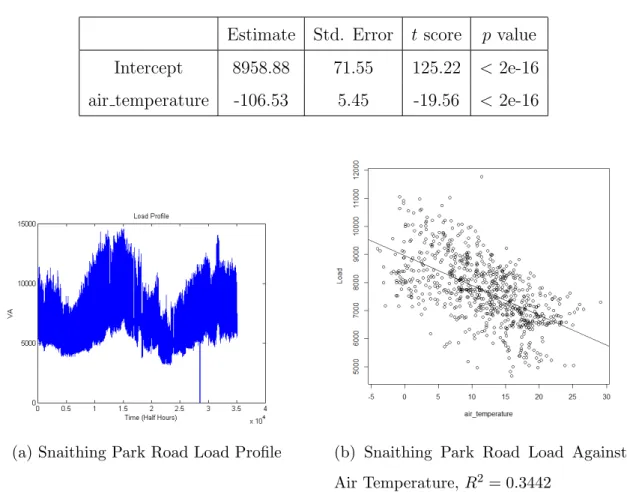
4.1.4 Snaithing Park Road - Yorkshire . . . 62
4.1.5 Durkar Low Lane - Yorkshire . . . 63
4.1.6 Comments on Data Quality . . . 64
4.1.7 Conclusions on Air Temperature Data . . . 64
4.2 Output Area Classification . . . 65
4.2.1 Experiment with OAC . . . 67
Contents xv
4.2.3 Na¨ıve Bayes Classification . . . 70
4.2.4 Conclusions on OAC Classification . . . 71
4.3 Customer Information by NPG . . . 71
4.3.1 Introduction and Related Work for Customer Information . . 72
4.3.2 Data Set Description . . . 73
4.3.3 PCA Overview . . . 75
4.3.4 K-Means Clustering Overview . . . 76
4.3.5 Comparing Monthly Growths . . . 77
4.3.6 Usage of Principal Component Analysis . . . 77
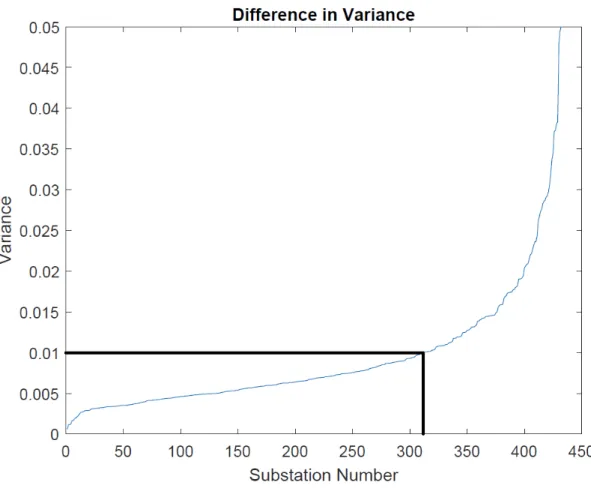
4.3.7 Adjustment of threshold value and error metrics . . . 82
4.3.8 Conclusions on NPG Customer Information . . . 85
4.4 Conclusion . . . 86
5 Methods for Analysing Substation Demand Data 87 5.1 Consideration of Maximum Demand and Outlier Detection . . . 88
5.1.1 Automated Maximum Demand Selection . . . 88
5.1.2 Wavelet based outlier detection . . . 92
5.1.3 Usefulness of Kurtosis Flag . . . 95
5.1.4 Comparison of Methods . . . 95
5.1.5 Initial Look at Load Transfers . . . 97
5.2 Base Load Profile Determination . . . 101
5.2.1 Median Replacement . . . 101
5.2.2 Updated Load Transfer Algorithm and Shift Technique . . . . 104
5.3 Conclusion . . . 114
6 CL-ANFIS Forecasting Algorithm 115 6.1 Motivations for CL-ANFIS . . . 116
6.2 Theory and Methods Used . . . 117
6.2.1 Creation of Representative Load Profiles . . . 118
6.2.2 ANFIS . . . 132
6.2.3 Benchmark - Holt-Winters Exponential Smoothing . . . 135
Contents xvi
6.4 Results of Clustering Method . . . 138
6.4.1 Clusters 2 and 4 - The “Traditional” Load Profiles . . . 139
6.4.2 Cluster 5 - The Non-Peaked Load Profile . . . 141
6.4.3 Clusters 6 and 7 - The Flat Load Profiles . . . 141
6.4.4 Comments on the Remaining Clusters . . . 142
6.4.5 Comparison of the CL-ANFIS Model against Holt-Winters . . 142
6.4.6 Summary of Results . . . 143
6.5 Analysis of Forecast Errors Using Demographic Information . . . 143
6.6 The Qualitative Importance of CL-ANFIS . . . 147
6.7 The Impact of the Customer Classifications on Load Profiles . . . 151
6.7.1 Data Description . . . 151
6.7.2 Methodology and Experiment . . . 153
6.7.3 Overall Algorithm Results . . . 155
6.7.4 K-Nearest Neighbours . . . 156
6.7.5 Na¨ıve Bayes Results . . . 159
6.7.6 Decision Tree Results . . . 162
6.7.7 Comparing Methods . . . 163
6.8 Conclusion . . . 164
7 Evaluation and Testing 166 7.1 Examination of Daily Load Profile Clusters . . . 166
7.2 Evaluating CL-ANFIS with Subset Input Data . . . 170
7.2.1 Method for CL-ANFIS Evaluation with Subset Input Data . . 170
7.2.2 Results and Discussion of CL-ANFIS Evaluation with Subset Input Data . . . 171
7.3 Comparison against NPG DLEs . . . 174
7.3.1 Method for Comparsion against NPG DLEs . . . 174
7.3.2 Results and Discussion of NPG Comparison . . . 175
7.4 Conclusion . . . 178
8 Conclusions 179 8.1 Addressing Research Questions . . . 179
Contents xvii
8.1.1 RQ1: Internal Factors . . . 180
8.1.2 RQ2: External Factors . . . 180
8.1.3 RQ3: Transparency of Information . . . 181
8.1.4 RQ4: Enhancing Business as Usual for NPG . . . 182
8.1.5 RQ5: Evaluation of CL-ANFIS Method . . . 183
8.2 Recommendations for Future Works . . . 183
8.2.1 Adjustment of the Current Method . . . 184
8.2.2 Consideration of Future Data . . . 184
8.2.3 Alternative methodologies . . . 185
Bibliography 185
Appendix 197
List of Figures
1.1 Projected Energy Demand and Supply in 2050 by DECC
(Depart-ment of Energy and Climate Change, 2010) . . . 5
1.2 Map of the DNO Areas in the UK with NPG operating in Area 5 (Energy Networks Association, 2014) . . . 7
2.1 UK Electrical Distribution Network Diagram (EDW Technology, 2017) 13 2.2 Sample Load Duration Curve . . . 18
2.3 Choice of MD in Various Scenarios (CE Electric UK, 2009) . . . 19
2.4 Acceptable Forecast Tolerance Opinions . . . 24
3.1 ANFIS Architecture . . . 42
4.1 Potter House Substation Investigation, April 2011 - March 2013 . . . 60
4.2 Scarborough 11kV Substation Investigation, April 2011 - March 2013 61 4.3 Snaithing Park Road Substation Investigation, April 2011 - March 2013 62 4.4 Durkar Low Lane Substation Investigation, April 2011 - March 2013 . 63 4.5 OAC Methodology (Office for National Statistics, 2015) . . . 66
4.6 Difference in Error Variance between Substation Trend and National Trend . . . 78
4.7 Scree Plot of Variance Explained by Principal Components . . . 79
4.8 K-Means Clustering of PC Space . . . 80
4.9 Substations which Deviate from National Trend . . . 81
4.10 Difference between Load Profiles in Principal Component 1 . . . 82
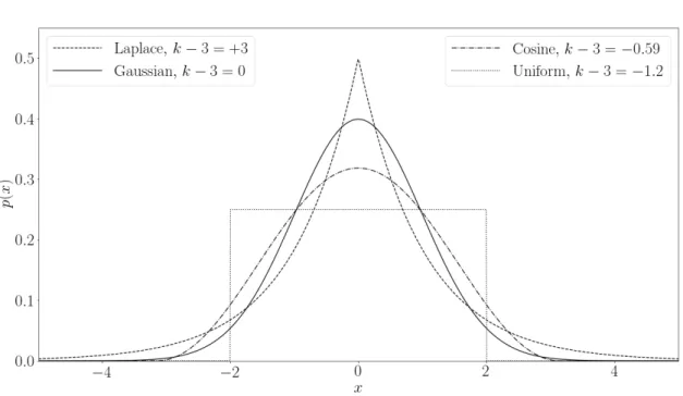
5.1 Example of Distributions with Positive and Negative Kurtosis Values (Ivezi´c et al., 2014) . . . 90
List of Figures xix
5.2 Abbey Road Annual Load Profile with Maximum Demand in Green . 91
5.3 Abbey Road Daily Load Profile with Outliers Indicated . . . 91
5.4 Yorkshire Load Profile Kurtosis Values . . . 95
5.5 Yorkshire MD Error Distribution Between NPG DLE MD and Auto-mated Method . . . 97
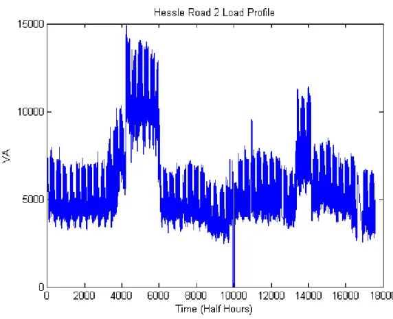
5.6 Hessle Road 2 Load Profile . . . 98
5.7 2011 Arundel Street Load Profile after Outlier Detection . . . 104
5.8 Network Diagram Around Arundel Street . . . 107
5.9 Percentage Change in Kurtosis for 2 years . . . 108
5.10 Percentage Change in Kurtosis for 2011/12 . . . 109
5.11 Percentage Change in Kurtosis for 2012/13 . . . 109
5.12 Percentage Change in Kurtosis for 2 years Using Raw Data . . . 110
5.13 Percentage Change in Kurtosis for 2011/12 Using Raw Data . . . 111
5.14 Percentage Change in Kurtosis for 2012/13 Using Raw Data . . . 111
5.15 Percentage Change in Kurtosis for 2 years Using Combined Approach 112 5.16 Percentage Change in Kurtosis for 2011/12 Using Combined Approach113 5.17 Percentage Change in Kurtosis for 2012/13 Using Combined Approach113 6.1 Dunn’s Index for Crisp Clustering Algorithms . . . 121
6.2 DB Index for Crisp Clustering Algorithms . . . 122
6.3 Xie-Beni Index for Fuzzy C-Means . . . 123
6.4 Clusters Gained By K-means With K=9 . . . 124
6.5 Clusters Gained By Hierarchical Clustering . . . 126
6.6 Clusters Gained By Fuzzy C-means Clustering . . . 128
6.7 Membership Function Example . . . 134
6.8 Flowchart for CL-ANFIS Model . . . 136
6.9 Difference between Load Profiles in Principal Component 1 . . . 140
6.10 Subclusters of Clusters 6 and 7 . . . 146
6.11 Summer Clusters Gained By K-means With K=9 . . . 152
6.12 Winter Clusters Gained By K-means With K=9 . . . 153
6.13 Scatter Plot of Number of Domestic 1 Customers against Number of Office & Admin Customers with Class1S labels . . . 157
List of Figures xx
6.14 PDFs of Office & Admin Customers . . . 160 7.1 Silhouette Plot for Daily Load Profile Clusters . . . 167 7.2 Median MAE values of Robustness Evaluation for CL-ANFIS . . . . 172 7.3 Median RMSE values of Robustness Evaluation for CL-ANFIS . . . . 173 A.1 Cluster 1 Substation Daily Load Profiles with Postive and Negative
Silhouette Values Highlighted . . . 198 A.2 Cluster 2 Substation Daily Load Profiles with Postive and Negative
Silhouette Values Highlighted . . . 198 A.3 Cluster 3 Substation Daily Load Profiles with Postive and Negative
Silhouette Values Highlighted . . . 199 A.4 Cluster 4 Substation Daily Load Profiles with Postive and Negative
Silhouette Values Highlighted . . . 199 A.5 Cluster 5 Substation Daily Load Profiles with Postive and Negative
Silhouette Values Highlighted . . . 200 A.6 Cluster 6 Substation Daily Load Profiles with Postive and Negative
Silhouette Values Highlighted . . . 200 A.7 Cluster 7 Substation Daily Load Profiles with Postive and Negative
Silhouette Values Highlighted . . . 201 A.8 Cluster 8 Substation Daily Load Profiles with Postive and Negative
Silhouette Values Highlighted . . . 201 A.9 Cluster 9 Substation Daily Load Profiles with Postive and Negative
List of Tables
2.1 DLE Growth Rates for Substation Categories . . . 22 2.2 MAPE for One Year Ahead Forecasts (CE Electric UK, 2009) . . . . 23 2.3 MAPE for Two Year Ahead Forecasts (CE Electric UK, 2009) . . . . 23 4.1 Summary Information of Potter House Temperature Regression . . . 59 4.2 Summary Information of Scarborough Temperature Regression . . . . 61 4.3 Summary Information of Snaithing Park Road Temperature Regression 62 4.4 Summary Information of Durkar Low Lane Temperature Regression . 63 4.5 Overall Decision Tree Errors . . . 69 4.6 Decision Tree Training Misclassifications . . . 69 4.7 Overall Na¨ıve Bayes . . . 70 4.8 Na¨ıve Bayes Training Misclassifcations . . . 71 4.9 Domestic Housing Definitions . . . 74 4.10 Substations that Matched Trend by Cluster . . . 80 4.11 Confusion Matrix . . . 83 4.12 Error Metrics for 30% Proportion [NaN is undefined] . . . 84 4.13 Error Metrics 50% Proportion [NaN is undefined] . . . 84 4.14 Error Metrics 70% Proportion [NaN is undefined] . . . 85 5.1 Confusion Matrix Values for Sigma Threshold Parameters . . . 100 6.1 K-Means Clustering Populations and Principal Component Values . . 123 6.2 Hierarchical Clustering Populations and Principal Component Values 126 6.3 Clusters Gained By Fuzzy C-means Clustering . . . 129 6.4 Median Errors of Three Forecasting Models . . . 139
List of Tables xxii
6.5 Weighted Similarity Measure . . . 139 6.6 Variance of Principal Components per Cluster . . . 144 6.7 Low Customer Substations and their Forecasting Error . . . 145 6.8 Maximum Demand Values across Clusters . . . 147 6.9 Qualitative Descriptors . . . 148 6.10 Frequency of a and c parameters . . . 149 6.11 Average Distribution of Load forc Parameter . . . 150 6.12 Summer Classification Labels . . . 152 6.13 Winter Classification Labels . . . 153 6.14 Classification Method Errors for Summer . . . 155 6.15 Classification Method Errors for Winter . . . 155 6.16 KNN Errors for Summer . . . 156 6.17 KNN Errors for Winter . . . 156 6.18 Na¨ıve Bayes Errors for Summer . . . 159 6.19 Na¨ıve Bayes Errors for Winter . . . 159 6.20 Decision Tree Errors for Summer . . . 161 6.21 Decision Tree Errors for Winter . . . 162 7.1 Average Variance of Daily Load Profile Cluster Values . . . 168 7.2 Average Variance of Daily Load Profile Cluster Values After Negative
Silhouette Values are Removed . . . 169 7.3 Median MAE values of Robustness Evaluation for CL-ANFIS
[Aver-ages based on 10 different random initialisations] . . . 171 7.4 Median RMSE values of Robustness Evaluation for CL-ANFIS
[Av-erages based on 10 different random initialisations] . . . 171 7.5 Median Percentage Errors for MD Forecast . . . 176 A.1 Reordering of K-Means Clusters . . . 197
Chapter 1
Introduction
Northern Powergrid (NPG) is an electrical distribution network operator (DNO) which services many types of customers throughout Yorkshire and the North East of England. Electrical demand data is collected using SCADA (Supervisory Control and Data Acquisition) facilities at frequent intervals of every 30 minutes. This in-formation is summarised in the DLEs (Distribution Load Estimates) documentation created by NPG but there remains underlying uncertainties which are not captured. Some of the uncertainties involved are included in the automated judgment of de-termining the annual maximum demand (MD). Even once the data is collected, its interpretation also raises uncertainties. For example, the impact of new demand or generation connections and when they would have an impact on the system. In the future, it will be important to not only have an accurate forecast of demand but also an informed forecast.
This thesis will create an informed forecast methodology using a combination of statistical and machine learning techniques to enhance the forecasting methodology by NPG.
1.1
Challenges Facing Northern Powergrid
NPG has provided the challenges and uncertainties they have with the SCADA data. Their primary difficulties are in establishing the MD figure which is used as the basis for demand forecasts in their current method.
1.1. Challenges Facing Northern Powergrid 2
1.1.1
Uncertainties With the Raw SCADA Data
Firstly, there are uncertainties regarding issues with the raw SCADA data including the following:
• The selection of MD for input on the DLEs is a key uncertainty. This assess-ment is done through an automated method but involves a lot of engineering judgment as well. This is examined in greater detail in Chapter 2.
• These are also temporary demand transfers where load is shifted from one substation to another in order to manage faults and network development. This is also examined in greater detail in Chapter 5.
• In the demand profile there are natural erratic demand peaks and generation troughs. Sometimes these peaks are ignored in the selection of MD but it is a subjective area where engineering judgment needs to be applied.
• There is natural variation in the demand itself with a variable accuracy of
±3%.
• SCADA equipment can produce erroneous data which can cause spikes or missing data for various time durations. If there are faults with the SCADA equipment, this can also lead to erroneous data.
1.1.2
Uncertainty in Interpreting the Raw Data
Regarding the interpretation of the data, new information can play a large role in modifying the forecast.
• New demand connections could of course lead to increased network demand. Although the capacity and date of energisation are known for a new customer, the rate at which they draw additional demand is unknown. This could po-tentially take years before they cause effect on the forecast.
• New generation connections could cause a decrease in net demand. Similarly to new demand connections, it can be unknown at times when the reduction would materialise in the demand profile.
1.1. Challenges Facing Northern Powergrid 3
• There may be reduced demand or disconnections from existing customers. This would lead to a decrease in demand but it is not identifiable whether such demand reduction or disconnection is temporary or permanent.
• In the past Average Cold Spell Correction (ACS) was used to normalise net-work demand for temperature. The aim of ACS is to account for variations in demand caused by temperatures in the winter period. However, NPG does not currently use ACS as there were concerns that it introduced errors. Further details are given in Chapter 2.
• The diversity factor is the ratio of the MDs of the supply point substation against the aggregated MDs of the primary substations. It is possible for the MDs at the satellite substations to increase while the demand at the source substation decreases due to the reduced co-incidence of the demand profile peaks at the satellite substations.
• The power factor varies throughout the year but the one recorded in the DLEs is taken to be the power factor at the time the MD occurred.
1.1.3
Future Uncertainties
This thesis is aimed at understanding the historical demand. However, NPG has outlined some areas in which some uncertainties will need to be understood in order to be able to incorporate them into the forecasting process.
• Energy prices will drive energy usage. For example, consumers may take greater advantage of energy reduction initiatives and use equipment which is more efficient.
• The DNO may introduce time of use tariffs to reduce peak demands. There will be a need to understand how effective these tariffs are at reducing demand.
• The introduction of smart metering is also expected to have an impact on de-mand measurement and forecasting methodologies. More data should be avail-able from customers which will move the methodologies away from a planning
1.2. Current Challenges in Long-Term Demand Forecasting 4
based approach towards a real time operational approach. Although there will still need to be a governance structure in place for reinforcement on the network.
Some of these uncertainties will be addressed in the proposed forecasting method such as when dealing with missing data from SCADA equipment. Other issues such as uptake of demand from a new customer or the impact of smart grids will not be considered as they are outside the scope of this work.
1.2
Current Challenges in Long-Term Demand
Forecasting
The need to understand the historic demand data for NPG and other DNOs is in-fluenced by the quickly changing landscape in energy usage and how energy demand data will be collected.
In particular, the Department of Energy and Climate Change (DECC) has de-tailed future energy pathways in the 2050 Pathways Analysis (Department of Energy and Climate Change, 2010). At the time of this writing, note that DECC was dis-solved in July 2016 and was merged with the Department for Business, Innovation and Skills (BIS) to form the Department for Business, Energy and Industrial Strat-egy (BEIS). This analysis was done as a result of climate change and an initiative to reduce greenhouse gas emissions by at least 80% by 2050 in comparison to 1990 levels. In Fig. 1.1, the breakdown of pathways is detailed in terms of the supply and demand from each sector.
On the left of the bar chart is the reference pathway labelled “R”. This represents a scenario where there is no attempt to decarbonise and no new energy technolo-gies are deployed. It is clear to see that the diversity of energy supply sources is non-existent in comparison to the pathways A-F. These all represent scenarios with various attitudes and uptake of certain energy technologies. For example, pathways “A” represents a substantial cross-sector effort to decarbonise while pathway “D” represents a scenario where there is very little uptake of renewable energy. For the
1.2. Current Challenges in Long-Term Demand Forecasting 5
Figure 1.1: Projected Energy Demand and Supply in 2050 by DECC (Department of Energy and Climate Change, 2010)
base case of 2010 when this study was conducted, supply was comparable to refer-ence pathway except with some proportion of nuclear energy. The demand in 2010 was also similar to the reference pathway but with a reduced demand for heating
1.2. Current Challenges in Long-Term Demand Forecasting 6
and cooling ( 200 TWh/year) (Department of Energy and Climate Change, 2010). The losses given in the supply bar chart are relative to the scenarios they are in. For example, pathway “D” is the low renewables scenario resulting in an increased up-take of nuclear energy which also leads to higher energy losses. Conversely, pathway “C” represents a scenario with little nuclear uptake resulting in much lower energy losses.
As there are many uncertainties about the type of technologies that will be used in the future, a scenario based approach like this is suitable for such a forward thinking analysis. There are many financial, political and socio-economical factors that contribute towards these pathways and considering each of them is complex.
So in general, understanding the drivers of national demand is extremely impor-tant because of the implications it will have on generation and emissions. NPG is one of the DNOs in the UK which covers the Yorkshire and Northeast regions of England as seen in Fig. 1.2.
For the DNOs, there are a variety of reasons for understanding historic demand and future forecasts. They have the requirement of meeting the contractual firm capacity at substations but they also are exploring other avenues of innovation. In order to address future energy problems, NPG had the Customer-Led Network Revolution (CLNR) project (completed in 2014) (Northern Powergrid, 2016) which sought to find better alternatives to dealing with new demands on the network rather than the traditional approach of reinforcing the network. They did this through a smart grid technology trial for each of their customer sectors (domestic, small and medium-sized enterprises, industrial & commercial and distributed generation). They concluded that domestic customers can be flexible with their network usage and that they contribute less to network peak demand than originally assumed. For industrial and commercial customers, they concluded that demand side response is a reliable option in order to address network constraints.
Through this project, NPG have been able to develop tools that benefit other DNOs such as (Northern Powergrid, 2016):
• Network Planning Design and Decision Support tool
1.2. Current Challenges in Long-Term Demand Forecasting 7
Figure 1.2: Map of the DNO Areas in the UK with NPG operating in Area 5 (Energy Networks Association, 2014)
• Lessons learned reports
• “How to” guidelines for equipment and training
The changing landscape in energy supply and demand is driving the research done in this thesis and in other related projects (National Grid, 2013; Northern
1.3. Research Questions 8
Powergrid, 2016; Western Power Distribution, 2013). In order to better meet the energy demands of the future, it is clear that a substantial amount of research must be undertaken to meet those needs.
1.3
Research Questions
Some key research questions can be developed based on the challenges NPG are facing and the current state of research in the electrical distribution forecasting area. The following key research questions (RQ) are laid out here which will be addressed in future areas of the thesis with a final discussion in the concluding Chapter 8.
RQ1: How can statistical and machine learning methods be used to analyse internal factors such as demand variation?
Justification: This is directly related to the challenges facing NPG currently
including the uncertainties within the raw SCADA data in Section 1.1.1. RQ2: How can statistical and machine learning methods be used to analyse external
factors such as temperature and customer type?
Justification: This is one of the key drivers for NPG in terms of gaining a
better understanding of their network. This has already influenced projects such as the CLNR and external factors are a natural extension for this work as well.
RQ3: How can more transparency be gained about current and future trends after analysing internal and external factors?
Justification: In particular, NPG requires methods where a qualitative
expla-nation can be derived from the results rather than a pure black box technique. RQ4: How can the forecast and insights gained from statistical analysis be used to
enhance the business as usual for NPG?
Justification: In particular, NPG needs to be able to practically use the
method in such a way that it can be implemented into their current architec-ture.
1.4. Research Contributions 9
RQ5: How can an evaluation of a new method be conducted, given the multiple influencing factors which affect the load?
Justification: There needs to be a level of evaluation to justify the use of the
new method by NPG and it must be conducted on every main component of the method.
1.4
Research Contributions
The purpose of the project is to not only develop a method which is capable of forecasting demand but also to develop a greater understanding of the underlying substation demand trends from data that is routinely collected from SCADA and other data systems. This is done with a desire to form a more informed and robust view of the required load related investment. Currently, NPG has a system which handles data directly from SCADA systems without any supplementary analysis input into the forecast. If there is a fault or unexpected load on the system, it is dealt with on a case-by-case basis. New connections and generation are considered but underlying drivers of electrical demand such as weather, economic conditions, and demographic information are not considered. Therefore, the goal is to have a more robust understanding of the most influencing factors on demand and using this information to supplement and enhance a forecasting tool.
This has been addressed in the original contribution CL-ANFIS (Customer-Led ANFIS). With this method, NPG have a more robust method where the generated forecast is supported by customer segmentation using machine learning techniques. This allows for a greater understanding of demand on substation-by-substation basis. They can implement these methods through a combination of the code produced in MATLAB and Excel spreadsheets such that it can run in a Windows environment. As of this writing, the methodology will be delivered to NPG for trial use.
In addition, a novel approach to NPG’s MD selection method is presented in Chapter 5. This presents an automated method which removes the necessity for NPG engineers judgement in choosing a MD for the current year. In addition to the potential time saving and reduction in bias, this method also forms the basis for
1.5. Structure of Thesis 10
testing in Chapter 7. Chapter 5 also explores an approach to handling load transfers which can have an unwanted effect on the determination of maximum demand and forecasting in general.
1.5
Structure of Thesis
In this chapter, the motivation for the current research has been introduced and the contributions of the thesis have been outlined. The structure of the following chapters are as follows.
Chapter 2 (RQ1, RQ2) will explicitly describe the current NPG practice in their determination of MD, forecasting and historic research they have performed. In particular it will examine their documentation which describes their methods and preliminary research NPG has conducted. This will give further motivations for this research and background for the problem.
Chapter 3 (RQ1, RQ2, RQ3) is a more general literature review discussing the current techniques used in data mining and time series analysis with applications in multiple industries. The approach here is to present both the most commonly used methods in time series and machine learning analytics as well as direct applications of those tools. In this way, a wide variety of areas are covered for use in this thesis and future work.
Chapter 4 (RQ2) explores additional data sets that could be used in conjunction with the informed demand forecasting method. This includes temperature data from the Met Office, demographic information from publicly available sources and in-house demographics from NPG.
Chapter 5 (RQ1) details some of the methods used in cleaning the original SCADA data set and the automated MD selection method. This process is cen-tral prior to the use of ANFIS as any missing data or erratic spikes can have an unwanted effect on the forecast. It is also important to have an automated method of choosing MD such that a comparison against current NPG methods can be made. Chapter 6 (RQ3, RQ4, RQ5) details the CL-ANFIS methodology with initial results following forecasting on available data. The bulk of the proposed method is
1.5. Structure of Thesis 11
reported here and in addition, there is an analysis of the customer types by their proposed quantitative labels.
Chapter 7 (RQ5) deploys further evaluation techniques to check the algorithm for robustness and compares the method to current NPG practices. The comparison to the NPG forecast is done in a similar way using MDs so that a direct comparison of forecasting aspect of CL-ANFIS can be made.
Chapter 8 concludes the thesis by discussing the findings and proposes further work and other avenues that could be explored.
Chapter 2
The Current Northern Powergrid
Method
In order to address the forecasting problem, this chapter will explore the current methods used by NPG as well as older research they have conducted on their current procedures. The forecasting problem is a result of both underlying uncertainties such as the collection of raw load data and data interpretations. For example, new load and generation connections can cause changes in demand and thus a change in the forecast. In Section 2.1, a brief overview of NPG and its role as a distribution company is given. Section 2.2 explains some of the motivations for the creation of a Load Related Investment Plan by NPG. Section 2.3 explains the NPG method in greater detail including some of their own research on the effectiveness of their method. Section 2.4 concludes with the findings of the NPG method.
2.1
The Role of Northern Powergrid in Electricity
Distribution
Energy distribution in Great Britain is conducted by one of the 14 DNOs which are owned by six companies. One of these companies and the sponsor of this research is NPG. The transmission of electricity is conducted solely by the National Grid. National Grid and the DNOs are subject to the rules and regulations set by industry
2.1. The Role of Northern Powergrid in Electricity Distribution 13
regulator OFGEM. In addition to transmission and distribution, there are also the supply companies of electricity which pay the National Grid and DNOs for use of their assets to deliver energy to individual customers.
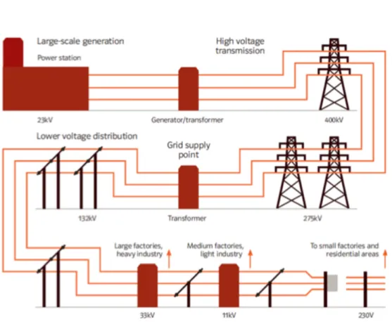
Figure 2.1: UK Electrical Distribution Network Diagram (EDW Technology, 2017)
For the purposes of this research, the focus will be on energy demand as viewed by DNOs. Fig. 2.1 shows a diagram of the UK distribution network. The National Grid transmits electricity at the 400kV and 275kV levels. These are then stepped down to the 132 kV sub-transmission level which is the first level operated and owned by the DNOs. DNOs own sites known as Grid Supply Points (GSPs) which are connected to the National Grid (Northern Powergrid, 2015). These GSPs typically operate at this 132 kV level and form the highest layer of the total DNO network.
The 132 kV sub-transmission level is then stepped down to 66/33 kV levels which are classified as extra high voltage (EHV). These are often large industrial customers which will have their own transformer.
The primary substations which are the main focus of this research operate at medium voltage levels of 20/11/6.6 kV. The most common are the 11 kV substations
2.1. The Role of Northern Powergrid in Electricity Distribution 14
which are reached by stepping down from the 132 kV or EHV levels. Although distribution to individual residential users at the 240 V level is outside the scope of this research, the types of customer the primary substations serve is key in gaining a deeper understanding of load demand.
2.1.1
Definitions and Basic Overview of Northern
Power-grid Method
NPG collects demand data from a SCADA (Supervisory Control and Data Acquisi-tion) system which is collected in a data historian called PI (CE Electric UK, 2009; OSIsoft, 2017). This is done for all the substations they operate and is recorded in voltage-amperes (VA). This is due to measuring the apparent power |S| on an alternating current power system as |S| = |V||I| = pP2+Q2 where P is the real power and Q is the reactive power (IEEE, 2000). The complex power S in phasor form as a function of the apparent power|S|is given asS =|S|∠ψ =P +jQwhere
ψ is the angle of difference between voltage and current. Although not an SI unit, apparent power is typically used as a power rating as it is simply the product of RMS (root-mean-square) voltage and RMS current (IEEE, 2000). Each substation will have a firm capacity associated to them which is the contractually agreed upon amount of load NPG must be able to supply to the customer. This figure is supple-mented by a MD and a load forecast of the MD. The MD is the maximum recorded load at a substation subject to certain conditions (see Section 2.3.1) which is fore-casted on over an eight year period. If the agreed upon firm capacityDis exceeded for that substation during the load forecast period, then some work on that part of the network must occur (see Section 2.2). That is, for any given substation with MD d0 in the current DLE year and forecast MDs di for i= 1,2, ...,8, then di < D must be satisfied for alli= 0,1, ...,8. Associated with this is the concept of network risk which can be defined as the frequency of interruptions to a customer at a site (Kaplan, 1990). The composite risk index specific to NPG is discussed in Section 2.2.
2.2. Load Related Drivers 15
2.2
Load Related Drivers
Before detailing the DNO method and past experiments, it is important to consider NPG’s drivers related in developing their Load Related Investment Plan. Namely, the distribution network must have the capacity to support customer load. There are general requirements such as the Engineering Recommendation P2/6 (Scott, 2007) and the Electricity, Safety, Quality and Continuity Regulations 2002 (Wilson, 2002). These requirements help ensure that electrical distribution equipment is operable and meeting the purpose it was created for. NPG also has their own internal review for assessing network risk called the Composite Risk Index. The CRI places emphasis on substations which are operating over firm capacity. Substations which are over firm capacity are said to be the highest risk but there is also a consideration of the degree to which it is over firm capacity and the length of time over firm capacity. In addition there is a consideration of historic load demand. In particular, MD figures are used to determine if a rapid rate of growth indicates a high risk substation. Creighton (2011) also notes some areas where the CRI can be improved. Namely that there should be a consideration of the geographic distribution with a high CRI index. This would be useful in the instance of an outage where a load transfer may not be able to take place due to the unavailability of adjacent substations. Also there should be a consideration of the sensitivity of the current factors to determine if they should be weighted equally in the risk index. The key areas of interest for CRI factors according to Creighton (2011) are the derivation of MD, firm capacity, time over firm capacity and load forecasts.
The selection of MD is based on certain criteria and is not the absolute maximum. More stringent criteria for the selection of MD will increase the MD and subsequently increase the risk associated with the substation.
The selection of the firm capacity value is key in determining substation reinforce-ment. The firm capacity is dependent upon the rating of the equipment supplying the substation. However, in the cases of interconnected rings, the circuit may be the limiting factor so there needs to be a better understanding of the firm capacity taking into account interconnected ring circuits for related substations.
2.3. Northern Powergrid Methodology 16
factor in the CRI. Namely, the cyclic ratings of transformers can be affected. One way to deal with the over firm capacity substations is to perform short-term load transfers with low voltage transfer capacity for those substations that exceed the firm capacity by a significant amount.
Creighton identifies load forecasts as a factor for change in network risk. There-fore, this project will have a direct impact on how risk is currently assessed. Note that Creighton considers a scenario based forecast over a 20 year period as one pos-sible approach. For the purposes of the CRI, a broad approach such as this may be preferable although the DLEs consider an 8 year forecast.
Finally in Creighton (2011), there is a consideration of the intervention methods when reinforcement is required. Some of the traditional methods include:
• transformer replacements,
• change of network topology, and
• permanent/temporary transfer of load.
In the future, there will be a greater use of distributed generation in order to maintain a constant system performance. This is due to the increased uptake of renewables and technologies such as combined heat and power (CHP). In addition, smart techniques such as active network management can incorporate customer response to reduce demand as well as managing network assets (CE Electric UK, 2009). After understanding some of the motivations, a more detailed look at NPG’s load estimate process can be discussed.
2.3
Northern Powergrid Methodology
The primary reference for this section will be CE Electric UK (2009) as it is the main source which explicity describes the NPG forecasting method. The load estimate process is seen as the first stage of the integrated “end to end planning” process (CE Electric UK, 2009). The overall process takes input load data, produces observations and an 8 year ahead MD forecast in the DLEs. A first analysis of the data will
2.3. Northern Powergrid Methodology 17
identify any issues such as substations operating over firm capacity and solutions are proposed.
The DLEs and the overall process helps in compliance with certain license re-quirements. Every DNO must publish a long-term development statement under condition 25 of the distribution license (Gas and Electricity Markets Authority, 2017). In addition, the Grid Code (National Grid Electricity Transmission plc, 2017) requires the DNO to produce demand data at specific times for all grid sup-ply points (GSPs) and demand forecasts for the next 7 years.
In section 2.3.1, the determination of MD is discussed. Section 2.3.2 examines how ACS was implemented in the past. Section 2.3.3 dicusses underlying growth rates in the NPG forecast process. Section 2.3.4 discusses adding large load changes due to new connections. Section 2.3.5 explains the documentation known as the DLE. Section 2.3.6 detail the problems considering by NPG in the load estimate process.
2.3.1
Determination of Maximum Demand
The current NPG method is based around the determination and forecasting of the MD figure. The MD figure is defined as (CE Electric UK, 2005):
The highest value of demand recorded in any half hour at the metered point of connection with the NPG network under normal system opera-tion and configuraopera-tion condiopera-tions.
After the half hourly demand is extracted from the PI system, the MD is deter-mined based on the load duration curve. An example for a particular substation is given in Fig. 2.2. The load duration curve shows the number of half hourly periods
C(i) which fall above a particular load value.
Two variables are considered when choosing the MD. Let y be the absolute maximum, r ∈ [0,1] be a factor scaling the absolute MD to a new MD value, and
2.3. Northern Powergrid Methodology 18
Figure 2.2: Sample Load Duration Curve
the MD is:
min{ry when 15 total h values occur,
ry when 15 consecutive h values occur}
(2.3.1)
This is done to attain a reasonable MD value according to NPG based on other studies they have completed. The value of 15 was determined to be the most fit for purpose in internal studies at NPG. If the profile does not feature any discrepancies as in Fig. 2.3a then the MD value will be close to the actual peak. However, if there are any large erroneous spikes such in Fig. 2.3b, they are not considered in the MD determination. An exception to these cases occurs in Fig. 2.3c when there is a temporary load transfer for a period of a few weeks. This load transfer is also disregarded in the MD determination. In this instance, the load transfer does not accurately reflect the typical business as usual for that substation so any future planning should not take this into account. Once the MD is determined, the forecasting process begins.
2.3. Northern Powergrid Methodology 19
(a) Case I - Stable Profile
(b) Case II - Mostly Stable Profile with Erroneous Spikes
(c) Case III - Profile with a Load Transfer
Figure 2.3: Choice of MD in Various Scenarios (CE Electric UK, 2009)
2.3.2
Average Cold Spell Correction
ACS is an attempt to use temperature data to account for demand variation during the winter. ACS was used at NPG in the past but is no longer currently used. However, it is still important to understand how ACS was implemented in order to observe any impact temperature data had on the NPG method.
2.3. Northern Powergrid Methodology 20
stations. Therefore temperature data is not local to individual substations. The base winter temperature for ACS is −1.5◦C. Maximum demand is then increased or decreased dependent on the temperature difference away from−1.5◦C. The ACS correction equation is (CE Electric UK, 2009):
Macs =M + (0.7M(Te+ 1.5)) (2.3.2)
Te= 0.43T0+ 0.33T−1+ 0.24T−2 (2.3.3)
whereMacs is the ACS MD, M is the non-adjusted MD, Te is the effective temper-ature, T0 is the noon temperature on the day of MD, T−1 is the noon temperature on the day before MD and T−2 is the noon temperature two days before MD. As the temperature data is not local to each substation, there can be some variation in local temperatures versus the actual Met Office temperature data. This will result in variance of ±0.7% per ◦C difference up to maximum of 7.5%. Although there is no documentation for the coefficients values used here CE Electric UK (2009), based on the values of the coefficients for Te we can see that more recent days are weighted more heavily.
There have been instances in the DLEs where ACS was applied when the MD occurred in the summer even though it should only be applied for winter MDs. This resulted in a maximal 7.5% increased MD change for 106 substations in 2004. (CE Electric UK, 2009) theorises that MDs in summer months are a result of changes in energy usage such as:
• domestic use of gas for heat rather than electricity,
• reduction in initiatives to promote electricity usage through tariffs, and
• rise of air conditioning usage in commercial buildings.
It is noted that this change in energy usage, climate change and the overall impact of temperature on load data will have an impact on the uncertainty of ACS. Further work is discussed in Chapter 4 to determine the impact of temperature data on NPG substations.
2.3. Northern Powergrid Methodology 21
2.3.3
Load Forecasting for Underlying Growth
After the data has been extracted from PI and stored, growth rates are applied to the MD to produce the forecast. In the past, growth percentage forecasts were produced by using the following 5 sets of data (CE Electric UK, 2009):
1. Actual historic data
2. Actual historic consumption data
3. Cambridge Econometrics Industry Forecasts (Electricity, Gas, Water and Man-ufacturing) (Cambridge Econometrics, 2017)
4. Cambridge Econometrics Regional Forecasts (North East and Yorkshire and Humberside) (Cambridge Econometrics, 2017)
5. NG (National Grid) Seven Year Statement
This was found to be more effective at a high grid supply point level rather than at a primary substation level because of the way in which unit forecast data was split into five baskets of High, Low, Urban, Rural and EHV. The definitions with their associated load growth were originally the following (CE Electric UK, 2009):
• High - Substations situated in development areas receiving large numbers of enquiries and in significant large load blocks. 5% growth per annum
• Low - Substations situated in smaller planned development areas such as retail parks etc. 2% growth per annum
• Urban - Substations situated geographically in urban/suburban surroundings not subject to any specific local development. 0.5% growth per annum
• Rural - Substations situated geographically in rural surroundings not subject to any specific local development. 0.5% growth per annum
• EHV - EHV Customer owned substations, not affected by local development. 0% growth per annum
2.3. Northern Powergrid Methodology 22
However, the use of these five metrics “is not particularly scientific or documented” (CE Electric UK, 2009) and the “overall percentage growths are determined by using simple judgement without any calculations as such carried out.” (CE Electric UK, 2009) The documentation seems to be highly focused on gathering accurate fore-casting results with little consideration for how external metrics data could impact overall trends.
Table 2.1: DLE Growth Rates for Substation Categories YEAR HIGH LOW URBAN RURAL EHV
13/14 2.00 1.00 0.50 0.50 0.00
In the DLEs, the updated table of underlying growth percentage is presented as in Table 2.1. Although in actuality, the rates in Table 2.1 are not currently used. According to the code of practice (CE Electric UK, 2005), the overall demand growth varies little year to year and is usually in the order of 1%. Currently NPG only uses two underlying growth percentages: 0% for extra high voltage customers and 0.5% for all other primaries. While this choice is of small significance in the immediate 1-2 year future, these choices of underlying growth are more inaccurate for the 8 year forecasting horizon.
EA Technology (EA Technology, 2017) carried out an exercise to determine how effective NPG’s forecasting method was in comparison to just using a na¨ıve method of having the forecast for a year ahead be the actual value from the past year (CE Electric UK, 2009). In this assessment, only one year was tested despite a seven year ahead forecast being provided. This was due to the idea that the accuracy of the one year ahead forecast would affect future forecast years causing compounding errors. EA Technology used the previous years’ forecasted MD to make a comparison to the actual recorded MD value. The mean absolute percentage error (MAPE) was used as a uniform metric which would allow for comparison of a time series with small values against one with large values. It is given as:
M AP E = 1 n n X i=1 fi−ai ai (2.3.4)
2.3. Northern Powergrid Methodology 23
wheren is the total number of forecasts,fi are the forecasted MD values andai are the actual MD values. As a benchmark, a na¨ıve forecast was used which assumes the forecasted MD is the same as the actual MD from the previous year. The initial results on the sample substations are given in Table 2.2 and Table 2.3.
Table 2.2: MAPE for One Year Ahead Forecasts (CE Electric UK, 2009)
Base Year 00/01 01/02 02/03
Forecast Year 01/02 02/03 03/04 DLE Na¨ıve DLE Na¨ıve DLE Na¨ıve
Northeast 8.49% 6.53%
Yorkshire 8.56% 7.94% 8.98% 8.58%
Table 2.3: MAPE for Two Year Ahead Forecasts (CE Electric UK, 2009)
Base Year 00/01 01/02
Forecast Year 02/03 03/04 DLE Na¨ıve DLE Na¨ıve Yorkshire 12.62% 12.75% 11.33% 10.99%
These results show that either the na¨ıve approach performed better or there was a negligible difference between the methods. It is also noted that the usage of MAPE lead to discrepancies in terms of what is an acceptable error. The examples given in CE Electric UK (2009) are as follows:
Example 1 Example 2
Actual Demand = 3 MVA Actual Demand = 30 MVA Forecast Demand = 3.7 MVA Forecast Demand = 37 MVA Percentage Error = 23.33% Percentage Error = 23.33% Even though both examples have the same percentage error, only example 1 is considered an acceptable error while example 2 is not. This is due to the absolute difference in Example 2 being much larger than that of Example 1.
2.3. Northern Powergrid Methodology 24
Figure 2.4: Acceptable Forecast Tolerance Opinions
Fig. 2.4 (CE Electric UK, 2009) shows acceptable forecasting errors dependant on the MD based on four engineers’ opinions. Although there is some difference of opinion, it is clear that significantly higher forecast errors are acceptable at low MD values.
2.3.4
Forecasting Large Load Changes
In addition to the underlying forecast growth, the forecast demand is supplemented by large load changes of 1 MVA or above. Large loads are predicted to connect within the first year of the forecast. The information regarding new connections is not easy to establish so there are no hard rules where a new large load is certain to go ahead. There are many problems with the current information received from the connections process. NPG applies the load changes directly to the substation demand forecasts for the year they are due to come in.
An informal process of asking design engineers to detail any envisaged load trans-fers is carried out when forecasting large load transtrans-fers. In the process of determining MD, load transfers are often considered manually rather than using any defined
rule-2.3. Northern Powergrid Methodology 25
set. A data cleansing process of shifting load transfers should be used so they do not affect the forecasting tool. A historical look at the frequency of load transfers on particular substations could be investigated.
The generation data in the company is difficult to follow (CE Electric UK, 2009) because the demand used in the DLEs is the net result of the gross load connected to a substation. The incorporation of generation is treated similarly to the addition of new loads, the main difference being that only the net demand load is recorded. Since new generation could have an affect on forecasted load, they should be accounted for in some way but similar to new loads, only connections made in the short term are considered in the DLEs.
2.3.5
Distribution Load Estimate and Firm Capacity
The final stage involves recording the forecasted information in a user-friendly spreadsheet. The substations are grouped by their supply point substation. Each primary substation has the previous years actual demand along with a forecast for the next 8 years. Also recorded is the power factor and any connected generation at the primary substation. The supply point forecasts are created by aggregating all of the primary substations and applying a diversity factor calculated from the historical year. At the bottom of the sheet, existing generation is recorded along with any future large load or generation connections. The new large load changes are added directly to the 8 year forecasting period, usually within the first two years. Alongside each substation there is also a rating of the firm capacity. The firm capacity is typically defined as being the “amount of load that can be secured following the loss of the largest single item in that system.” (CE Electric UK, 2009) If load exceeds this firm capacity rating, then there is deemed to be a need for reinforcement at that particular substation. Most substations will have at least two transformers so defining the firm capacity to be one of those transformers is acceptable. For single transformer primary substations, firm capacity is routinely set at 8 MVA and design engineers confirm this is a known problem as this does not always accurately represent the firm capacity of the substation (CE Electric UK, 2009).
2.3. Northern Powergrid Methodology 26
2.3.6
Overall Load Estimate Process Problems
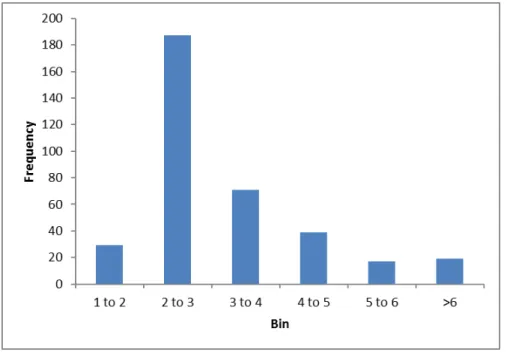
In the concluding sections of CE Electric UK (2009), some of the problems with the overall load estimate process were highlighted. With regards to the determination of MD values, some of the issues were discussed. Issues with the raw data are mentioned such as missing data and spikes, which can have a direct effect on MD determination. Regardless, it is stated that 35% to 50% of substations must be manually checked in the load estimate process every year. However, the aim is to always have some level of engineering judgment rather than a fully automated process. The engineering judgment is affected by the number of spikes in the profile and their duration. In their own studies, NPG found there is a correlation between the number of spikes beyond the perceived MD envelope and engineering judgment. This has led to the most recent definition of MD (CE Electric UK, 2009):
The highest value of demand recorded in any half hour under normal network feeding arrangements and taking into account of the impact of short duration high load values over a 12 month period.
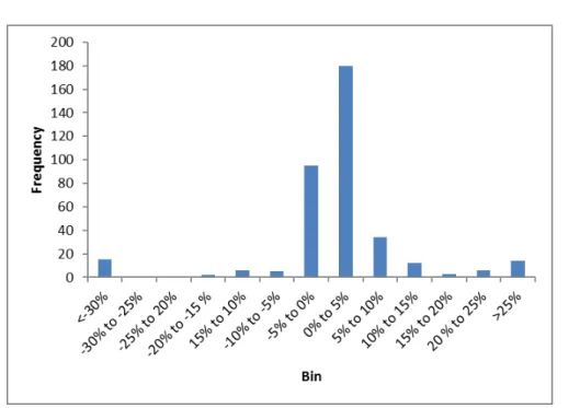
This correlates to the new method in Eqn. 2.3.1. Also discussed by CE Elec-tric UK (2009) were the underlying growth rates. EconomeElec-tric growth data is not available for site specific areas on a substation by substation basis. Growth rates for larger areas are available but they will mask regional trends. The issue that although overall system MD does not change greatly (in the order of 1-2%), pri-mary substation MD can vary greatly up to as much as±30%. Therefore, the focus should be on demand growth in the locality of each primary substation.
One suggested method would be to use new load enquiries as a basis for load growth. The relationship between new applications and demand growth could then be seen but this would require some new IT development in the current process. Another method would be to use substation growth categories as seen in Table 2.1. This would help to differentiate between substations with a flat load growth and those that are likelier to see change in load. Ultimately, these growth rates were not used but the idea of categorising substations in this manner is seen throughout the literature. The growth rates were not used because they did not accurately capture
2.4. Conclusion 27
the true variation at each substation.
2.4
Conclusion
This chapter has focused on documenting current and historical NPG practices for their overall forecasting method. In relation to the overall research questions for this thesis, it specifically relates to RQ1 and RQ2. That is, both internal and external factors have been considered by NPG and there are specific methods associated with both types. For example, their MD selection method as a consideration for an internal factor and Average Cold Spell correction for temperature data.
However, the purpose of this research is to not only develop a method which is capable of forecasting demand load but also to develop a greater understanding of the underlying substation demand trends from SCADA systems, with a view to forming a more informed and robust view of the required load related investment. Currently, NPG uses the PI system which handles data directly from SCADA sys-tems without any supplementary analysis input into the forecast. If there is a fault or unexpected load on the system, it is dealt with on a case by case basis. New connections and generation are considered but underlying drivers of electrical de-mand such as weather, economic conditions, and demographic information are not considered. Therefore, the goal is to have a more robust understanding of the most influencing factors on demand and using this information to supplement and enhance a forecasting tool.
Chapter 3
Techniques for Load Analysis
This initial literature review is conducted in the aim of discovering the current techniques and methods used in forecasting and trend analysis. This is done in accordance to satisfying both academic and commercial responsibilities with the goal of exploring techniques currently available and building upon them. This literature review sets out to follow a systematic approach suggested by Fink (2005) that can be reproduced in the future. In Section 3.1, the literature search method is detailed including the research questions. In Section 3.2, general techniques in machine learning will be explored. Section 3.3 will go over some examples of studies used in various industries and Section 3.4 will conclude and summarise the findings.
3.1
General Techniques in Machine Learning
Regardless of sector, much of the literature in data analysis uses common techniques in data mining and machine learning. Therefore it is important to introduce these ideas before looking at more specific examples. In this section, both supervised and unsupervised learning methods are introduced.
3.1.1
Supervised Learning
Supervised learning involves finding a function to describe a dataset with some input/output pair (xi, y) where xi are input features and y is the output feature to be learned. The main purpose of supervised learning will be to check if there is
3.1. General Techniques in Machine Learning 29
some clear relationship between datasets from NPG and any external data sources. For example, supervised learning can be used to establish if there is a connection between demographic data and substation demand.
Decision Trees
The decision tree is a data mining algorithm which gives a graphical representation of data classification. A data set is characterised by its attributes and class. Attributes are labels used to describe the characteristics of the data while the class is a special attribute that is used to identify the data point. The method operates by choosing the most appropriate attribute at each node of the tree based on various metrics. One such metric is information gain. Information gain is a measurement calculated from entropy which is a measure of uncertainty of a random variable. That is,
entropy(p1, ..., pn) = − n
X
i=1
pilog2(pi) (3.1.1)
wherepi is the probability of the event occurring (Hall et al., 2011). Entropy calcu-lations often use base 2 by convention and are measured in bits. It can intuitively be thought of a measurement of uncertainty because a high probability suggests low entropy and a low probability suggests high entropy. Along each branch, the algorithm will choose the attribute with the lowest entropy because it will result in the most correct classifications.
Decision trees provide a good intuitive visual representation of the data while also giving conditional statements along the branches. They are relatively quick to produce and do not require any domain knowledge or parameter setting. They are able to handle multidimensional data and are currently used in many industries including financial analysis, molecular biology, and medicine (Han et al., 2011).
Decision trees also have certain limitations. If proper precautions are not taken, they are prone to having high variance and can overfit to the training data. Small changes to the data or initial node can cause different trees to be constructed. In order to avoid this, methods such as tree pruning can be used. Tree pruning will cause the decision tree to be less accurate on the training data but more accurate on any unseen test data. Also, since decision trees handle one attribute at a time,
3.1. General Techniques in Machine Learning 30
this can lead to more inaccuracies. Two attributes that are almost equal in their discriminatory ability can lead to two different decision trees depending on which is used as the first node. However, taking the better attribute initially may not necessarily lead to a decision tree which is overall more accurate (Anderson, 2013).
Some popular applications of decision tree in the literature include:
• Friedl and Brodley (1997) used decision tree classifiers to classify remote sens-ing data sets for land cover classes such as forests, tundra and grasslands. It was found to be a useful tool for the data analysts as they are intuitive and useful for examining hierarchical relationships between the input data. The decision tree was also insensitive to noise and no assumptions are needed about the distribution of the data.
• Vlahou et al. (2003) used decision tree classification for diagnosis of ovarian cancer based on protein mass spectrum profiles. It was found to be 80% accu-rate when using five protein peaks although they state further preprocessing of the data could improve accuracy.
• Yu et al. (2010) used a decision tree method to estimate building energy per-formance indices. The results showed a 92% accuracy on the test data and was able to rank the significant factors of building energy usage. They also noted the interpretability of the method over regression techniques and neural networks.
K-Nearest Neighbours
<