A Model for Stock Price Prediction Using the Soft Computing Approach

(1)

A Model for Stock Price Prediction Using the Soft Computing

Approach

BY

ADEBIYI AYODELE ARIYO

(CU04GP0044)

A THESIS SUBMITTED IN PARTIAL FULFILMENT OF

THE REQUIREMENTS FOR THE AWARD OF

DOCTOR OF PHILOSOPHY DEGREE (Ph.D) IN

MANAGEMENT INFORMATION SYSTEM

OF THE DEPARTMENT OF COMPUTER AND

INFORMATION SCIENCES, COLLEGE OF SCIENCE AND

TECHNOLOGY COVENANT UNIVERSITY, OTA

NIGERIA

(2)

CERTIFICATION

This is to certify that this thesis is an original research work undertaken by Adebiyi

Ayodele Ariyo under the supervisions of Professors C.K Ayo and S.O. Otokiti and that the work has not been submitted for the award of any other degree in this or any other institution.

1. Name: Prof. Charles Korede Ayo

Supervisor

Signature: ___________________ Date:_____________

2. Name: Professor Sunday O. Otokiti

Co-Supervisor

Signature: ___________________ Date:_____________

3. Name: Professor Charles Korede Ayo

Head of Department

(3)

DECLARATION

It is hereby declare that this research was undertaken by Ariyo Ayodele Adebiyi. The thesis is based on his original study in the Department of Computer and Information Sciences, College of Science and Technology, Covenant University, Ota, under the supervision of Prof. C.K. Ayo and Prof. S.O. Otokiti. Ideas and views of this research work are products of the original research undertaken by Ariyo Ayodele Adebiyi and the views of other researchers have been duly expressed and acknowledged.

Professor Charles Korede Ayo Supervisor

Signature: ___________________ Date:_____________

Professor Sunday O. Otokiti Co-Supervisor

(4)

DEDICATION

This thesis is dedicated to God Almighty the Alpha and Omega of my life and also to my late grandmother for her unfathomable love and passionate desire that I succeed in life.

(5)

ACKNOWLEDGEMENTS

My deep appreciation goes to God Almighty; the Alpha and Omega of my life. I can see vividly His hand upon my life. He is always there for me in all situations. I appreciate greatly His priceless help and the wisdom He granted me throughout my doctoral studies. My profound appreciation goes to the Chancellor, Dr. David O. Oyedepo and the members of the Board of Regents of Covenant University for the Vision and Mission of the University. Also, special thanks to the Management staff of the University: the Vice Chancellor, Prof. Aize Obayan, the Registrar, Mr. J.N. Taiwo, the Deans of the Colleges, Prof. F.K. Hymore and Prof. K. Shoremilekun for their commitment to the pursuit of excellence and sound academic scholarship.

My appreciation goes to my supervisor, Professor Charles Korede Ayo for his untiring efforts, guidance, unconditional supports and immense contributions to the thesis. I equally want to thank him especially for his fatherly disposition to all his postgraduate students, his genuine concern both academically and spiritually. His leadership style is unparalleled and worthy of emulation. He is always interesting in providing opportunities for young academics, particularly those interested in Software Engineering and Intelligent System research. Many thanks goes to my co-supervisor, Prof. Sunday O. Otokiti, the former Head of Department of Business Studies at Covenant University, now the Dean of College of Business and Social Sciences, Landmark University, Omu-Aran for his enormous contributions, support and encouragement throughout the period of this study.

(6)

I also want to thank the Dean of College of Science and Technology, Prof. F.K. Hymore and Dean of Postgraduate Studies, Prof. C.O. Awonuga for their encouragement and support throughout the period of this study. I thank every member of staff of Department of Computer and Information Sciences for their support; in particular Dr. N.A. Omoregbe and Dr. J.O. Daramola for their contributions at the early stage of this study.

My appreciation goes to the Librarian for the useful materials obtained in the course of this work and the management of yahoo finance (http:/finance.yahoo.com) and cashcraft (www.cashcraft.com) for the live data used in this study.

I wish to appreciate the following people:. Firstly, my father, Elder Abiodun Adebiyi for his prayers and blessings in the course of this study and my brother and sister, Abayomi Adebiyi and Kehinde Adebiyi for their support and encouragement. Secondly, my in-laws, are wonderful people, in particular my mother-in-law, Mrs. Alice Ebun Owolabi, I am grateful to her for her prayers and support. Also, I appreciate my in-laws Dr. Henry Owolabi, Pastor Femi Owolabi and Pastor & Dr. (Mrs.) Olasehinde for their love and constant encouragement.

Finally, I am indeed grateful for the unflinching support of my beloved wife, Mrs. Marion Olubunmi Adebiyi for her love, encouragement and commitment to the success of this study. To my wonderful children, Ireoluwa Joy Adebiyi and Ayomide Iranwooluwa Joshua Adebiyi, thank you for being part of me and my success.

(7)

ABSTRACT

A number of research efforts had been devoted to forecasting stock price based on technical indicators which rely purely on historical stock price data. However, the performances of such technical indicators have not always satisfactory. The fact is, there are other influential factors that can affect the direction of stock market which form the basis of market experts’ opinion such as interest rate, inflation rate, foreign exchange rate, business sector, management caliber, investors’ confidence, government policy and political effects, among others.

In this study, the effect of using hybrid market indicators such as technical and fundamental parameters as well as experts’ opinions for stock price prediction was examined. Values of variables representing these market hybrid indicators were fed into the artificial neural network (ANN) model for stock price prediction.

The empirical results obtained with published stock data show that the proposed model is effective in improving the accuracy of stock price prediction. Also, the performance of the neural network predictive model developed in this study was compared with the conventional Box-Jenkins autoregressive integrated moving average (ARIMA) model which has been widely used for time series forecasting. Our findings revealed that ARIMA models cannot be effectively engaged profitably for stock price prediction. It was also observed that the pattern of ARIMA forecasting models were not satisfactory. The developed stock price predictive model with the ANN-based soft computing approach demonstrated superior performance over the ARIMA models; indeed, the actual and predicted value of the developed stock price predictive model were quite close.

(8)

TABLE OF CONTENTS Cover Page i Title Page ii Certification iii Dedication iv Acknowledgements v Abstract vii

List of Figures xii

List of Tables xvi

CHAPTER ONE: INTRODUCTION

1.1 Background of the Study 1

1.2 Statement of the Problem 6

1.3 Objectives of the Study 6

1.4 Research Methodology 7

1.5 Significance of the Study 8

1.6 Motivation for the Study 9

1.7 Contributions to Knowledge 9

1.8 Limitations of the Scope of Study 10

1.9 Organization of Study 10

CHAPTER TWO: LITERATURE REVIEW

2.1 Introduction 11

2.2 Background of Soft Computing Techniques 11

2.2.1 Artificial Neural Network 12

2.2.2 Fuzzy Logic 24 2.2.2.1Fuzzification 25 2.2.2.2 Inference Mechanism 26 2.2.2.3 Defuzzification 26 2.2.3 Evolutionary Computing 29 2.3 Statistical Techniques 34

(9)

2.4 Related Works of the Application of ANN in Stock Price Prediction 42

CHAPTER THREE: DESIGN AND DEVELOPMENT OF THE STOCK PRICE PREDICTIVE MODEL

3.1 Introduction 52

3.2 The Steps in Building ARIMA Model 53

3.2.1 Data Collection and Examination 53

3.2.2 Testing for Stationarity 54

3.2.3 Model Identification and Estimation 54

3.2.3.1 Box-Jenkins Methodology 55

3.2.3.2 Objective Model Identification 56

3.2.4 Model Diagnostics Checking 58

3.2.5 Forecasting and Forecast Evaluation 58

3.3 Model Development and Forecasting – ARIMA Model 60

3.3.1 ARIMA(p, d, q) Model Development for Stock Price of Dell

Incorporation 61

3.3.2 ARIMA(p, d, q) Model Development for Stock Price of Nokia

Incorporation 67

3.3.3 ARIMA(p, d, q) Model Development of Stock Price of Zenith

Bank 72

3.3.4 ARIMA(p, d, q) Model Development of Stock Price of UBA Bank 77

3.4 Steps in Designing ANN Forecasting Model 82

3.4.1 Variable Selection 82

3.4.2 Data Collection 83

3.4.3 Data Preprocessing 83

3.4.4 Training, Testing and Validation 83

3.4.5 Neural Network Design 84

3.4.6 Evaluation 84

3.4.7 Neural Network Training 84

3.4.8 Implementation 85

(10)

3.5.1 Backpropagation Neural Networks 85

3.5.2 Multi-layer Perceptron Model 87

3.5.3 Input Variables 88

3.5.4 Data Preprocessing 89

3.5.5 The Proposed Predictive Model 89

3.5.5.1 ANN Model Construction for Dell Stock Index 93

3.5.5.2 ANN Model Construction for Nokia Stock Index 96

3.5.5.3 ANN Model Construction for Zenith Bank Stock Index 99

3.5.5.4 ANN Model Construction for UBA Bank Stock Index 101

3.6 Performance Measures 104

3.6.1 Confusion Matrix 104

3.6.2 Statistical Method 105

3.7 Tools for Model Implementation 106

3.7.1 Matlab 106

3.7.2 Eviews 107

CHAPTER FOUR: RESULTS AND DISCUSSION

4.1 Introduction 108

4.2 ARIMA Model Results 108

4.2.1 Result of ARIMA model for Dell Stock Price Prediction 109

4.2.2 Result of ARIMA model for Nokia Stock Price Prediction 110

4.2.3 Result of ARIMA model for Zenith Bank Stock Price Prediction 112

4.2.4 Result of ARIMA model for UBA Bank Stock Price Prediction 114

4.3 ANN Model Results 116

4.3.1 Result of ANN model for Dell Stock Price Prediction 117

4.3.2 Result of ANN model for Nokia Stock Price Prediction 121

4.3.3 Result of ANN model for Zenith Bank Stock Price Prediction 125

4.3.4 Result of ANN model for UBA Bank Stock Price Prediction 129

(11)

CHAPTER FIVE: SUMMARY OF FINDINGS AND CONCLUSION

5.1 Introduction 134

5.2 Summary 134

5.3 Conclusion 136

5.4 Future Research Work 137

Appendix: LIST OF PUBLICATION 138

(12)

LIST OF FIGURES

Figure 2.1 Biological Neuron 16

Figure 2.2 Model of a neuron 19

Figure 2.3 An example of a simple feedforward network 20

Figure 2.4 A diagram of linear function 23

Figure 2.5 A diagram of tanh function 23

Figure 2.6 A diagram of the sigmoid function 24

Figure 2.7 Basic structure of an evolutionary algorithm 30

Figure 2.8 Schematic representation of a genetic algorithm 33

Figure 2.9 ARIMA forecasting procedure 42

Figure 3.1 Flowchart for building ARIMA model 61

Figure 3.2 Graphical representation of the Dell stock closing price index 62

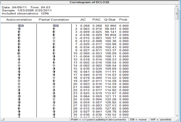
Figure 3.3 The correlogram of Dell stock price index 63

Figure 3.4 Graphical representation of the Dell stock price index after

Differencing 64

Figure 3.5 The correlogram of Dell stock price index after first differencing 64

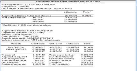
Figure 3.6 ADF unit root test for DCLOSE of Dell stock index 65

Figure 3.7 ARIMA (1, 0, 0) estimation output with CLOSE of Dell index 66

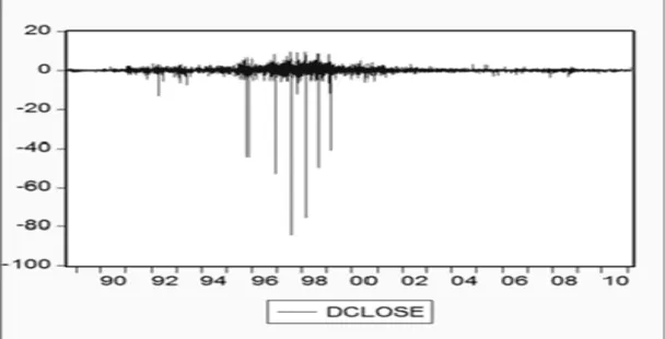
Figure 3.8 Graphical representation of the Nokia stock price index 67

Figure 3.9 The correlogram of Nokia stock price index 68

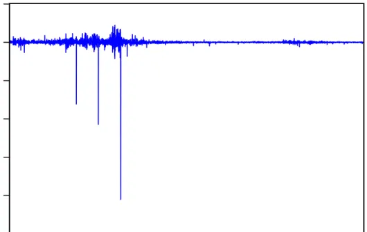
Figure 3.10 Graphical representation of the Nokia stock price index after

Differencing 69

(13)

Figure 3.12 ADF unit root test for DCLOSE of Nokia stock index 70

Figure 3.13 ARIMA (2, 1, 0) estimation output with DCLOSE of Nokia index 70

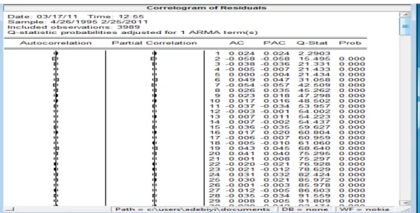
Figure 3.14 Correlogram of residuals of the Nokia stock index 71

Figure 3.15 Graphical representation of the Zenith Bank stock price index 72

Figure 3.16 The correlogram of Zenith Bank stock price index 73

Figure 3.17 Graphical representation of the Zenith bank stock index first

Differencing 73

Figure 3.18 The correlogram of zenith bank stock price index after first

Differencing 74

Figure 3.19 ADF unit root test for DCLOSE of Zenith bank stock index 74

Figure 3.20 ARIMA (1, 0, 1) estimation output with DCLOSE of Zenith bank

Index 75

Figure 3.21 Correlogram of residuals of the Zenith bank stock index 76

Figure 3.22 Graphical representation of UBA bank closing price of stock index 77

Figure 3.23 The correlogram of UBA Bank stock price index 78

Figure 3.24 Graphical representation of UBA bank stock index after

Differencing 79

Figure 3.25 The correlogram of UBA Bank stock price index after differencing 79

Figure 3.26 ADF unit root test for DCLOSE of UBA bank stock index 80

Figure 3.27 ARIMA (1, 0, 0) estimation output with DCLOSE of UBA bank

Index 80

Figure 3.28 Correlogram of residuals of the UBA bank stock index 81

(14)

Figure 3.30 Neural Network Architecture for Stock Prediction 92

Figure 3.31 Algorithm for ANN predictive model 92

Figure 3.32 Graph of best result achieved in network training of Model 1 of Dell

Index 95

Figure 3.33 Graph best result achieved in network training of Model 2 of Dell

Index 96

Figure 3.34 Graph of best result achieved in network training of Model 3 of Dell

Index 96

Figure 3.35 Graph of best result achieved in network training of Model 1 of Nokia

index 98

Figure 3.38 Graph of best result achieved in network training of Model 1 of Zenith

index 100

index 101

Figure 3.41 Graph of best result achieved in network training of Model 1 of UBA

(15)

index 103

Figure 4.1 Graph of Actual Stock Price vs Predicted values of Dell Stock

Index 110

Figure 4.2 Graph of Actual Stock Price vs Predicted values of Nokia Stock

Index 112

Figure 4.3 Graph of Actual Stock Price vs Predicted values of Zenith Bank Stock

Index 114

Figure 4.4 Graph of Actual Stock Price vs Predicted values of UBA Bank Stock

Index 116

Figure 4.5 Graph of Actual Stock Price vs Predicted values of Model 1 of Dell

Index 119

Index 120

Figure 4.8 Graph of Actual Stock Price vs Predicted values of Model 1 of Nokia

Index 123

(16)

Index 124

Figure 4.11 Graph of Actual Stock Price vs Predicted values of Model 1 of Zenith

Index 127

Index 128

Figure 4.14 Graph of Actual Stock Price vs Predicted values of Model 1 of UBA

Index 131

Index 132

(17)

LIST OF TABLES

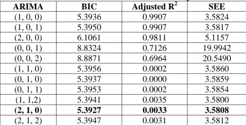
Table 3.1 Statistical results of different ARIMA parameters for Dell Stock

Index 67

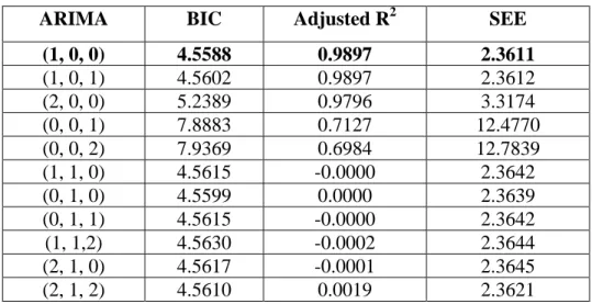
Table 3.2 Statistical results of different ARIMA parameters for Nokia Stock

Index 72

Table 3.3: Statistical results of different ARIMA parameters for Zenith bank Stock

Index 76

Table 3.4: Statistical results of different ARIMA parameters for UBA bank Stock

Index .82

Table 3.5 Eight steps in designing a neural network forecasting model 82

Table 3.6 Common parameters in designing BP networks for financial predictive

model 87

Table 3.7 Stock Variables (Technical Indicators) 88

Table 3.8 Stock Variables (Fundamental Indicators) 88

Table 3.9 Possible Stock Price Influence Factors (Experts Opinion) 88

Table 3.10 The Input and Output Parameters of the Models used in this Study 91

Table 3.11 Description of Input Variables used in this study 91

Table 3.12 Statistical performance of Mode 1 of Dell Stock index 94

Table 3.15 Statistical performance of Mode 1 of Nokia Stock index 97

Table 3.16 Statistical performance of Mode 2 of Nokia Stock index 97

(18)

Table 3.18 Statistical performance of Mode 1 of Zenith Bank Stock index 99

Table 3.21 Statistical performance of Mode 1 of UBA Bank Stock index 102

Table 3.24 A confusion matrix 104

Table 4.1 Sample of Empirical Results of ARIMA (1, 0, 0) of Dell Stock

Index 109

Table 4.2 Confusion matrix of predicted result of ARIMA model for Dell

Index 110

Table 4.3 Sample of Empirical Results of ARIMA (2, 1, 0) of Nokia Stock

Index 111

Table 4.4 Confusion matrix of predicted result of ARIMA model for Nokia

Index 112

Table 4.5 Sample of Empirical Results of ARIMA (1, 0, 1) of Zenith Bank

Index 113

Table 4.6 Confusion matrix of predicted result of ARIMA model for Zenith Bank

Index 114

Table 4.7 Sample of Empirical Results of ARIMA (1, 0, 0) of UBA Bank

Index 115

Table 4.8 Confusion matrix of predicted result of ARIMA model for UBA Bank

(19)

Table 4.9 Statistical performance of Mode 1-3 of Dell Stock index 118

Table 4.10 Sample of Empirical Results of ANN Models of Dell Stock Index 119

Table 4.11 Confusion matrix of predicted of ANN model for Dell Index 120

Table 4.12 Statistical performance of Mode 1-3 of Nokia Stock index 122

Table 4.13 Sample of Empirical Results of ANN Models of Nokia Stock

Index 123

Table 4.14 Confusion matrix of predicted of ANN model for Nokia Index 125

Table 4.15 Statistical performance of Mode 1-3 of Zenith Bank Stock index 126

Table 4.16 Sample of Empirical Results of ANN Models of Zenith Bank Index 127

Table 4.17 Confusion matrix of predicted of ANN model for Zenith Bank

Index 129

Table 4.18 Statistical performance of Mode 1-3 of UBA Bank Stock index 130

Table 4.19 Sample of Empirical Results of ANN Models of UBA Bank Index 131

Table 4.20 Confusion matrix of predicted of ANN model for UBA Bank

Index 133

(20)

CHAPTER ONE

INTRODUCTION

1.1

Background of the Study

The ability to accurately predict the future is crucial for decision processes in planning, organizing, scheduling, purchasing, strategy formulation, policy making and supply chains management and so on. Therefore, prediction/forecasting is an area where a lot of research efforts have been carried out in the past. This area is presently still an important and active field of human activity and will continue to be in the future (Zhang, 2004). Stock price prediction has always been a subject of interest for most investors and financial analysts, but clearly, finding the best time to buy or sell has remained a very difficult task for investors because there are other numerous factors that may influence

stock prices (Weckman et al., 2008, Chang and Liu, 2008 and Adebiyi et al 2009).

Therefore, stock market prediction has remained an important research topic in business. However, stock markets environments are very complicated, dynamic, stochastic and thus difficult to predict (Wei, 2005; Gerasimos et al., 2005; Yang and Wu, 2006; Tsanga et al., 2007; and Tae 2007).

Presently, financial forecasting is regarded as one of the most challenging applications of time series forecasting. Financial time series presents complex behaviour, resulting from a huge number of factors, which could be economic, political, or psychological. They are inherently noisy, non-stationary, and deterministically chaotic.

(21)

Data mining technology has found increasing acceptance in business areas that need to analyze large amounts of data in order to discover knowledge which could not be found using traditional methods. Time series data mining is identified as one of the 10 challenging problems in data mining research (Yang and Wu, 2006; Lay-Ki and Sang, 2007). Financial time series forecasting has been a subject of research since 1980s. The objective is to beat financial markets and win much profit. However, due to complexity of financial time series, there is some skepticism about predictability of financial time series. This is reflected in the well-known Efficient Market Hypothesis theory (EMH). According to the EMH theory, the current price is the best prediction for the next day, and buy-hold is the best trading strategy.

However, there are strong evidences which refuse the efficient market hypothesis (Pegal, 2007). Due to dynamic nature and unpredictable environment of stock market domain, predicting the future has always been the desire of mankind because of their inability to deal with uncertain, fuzzy, or insufficient data which fluctuate rapidly in very short periods of time. Artificial neural networks (ANNs) have become a very important method for stock market predictions (Schoeneburg, 1990). In recent years, soft computing techniques such as Artificial Neural Networks, Fuzzy Logic, and Genetic Algorithms have gained popularity for this kind of application. Much research efforts have been made to improve the predictive accuracy and computational efficiency of share values (Xiaodan Wu et al, 2001).

(22)

The elasticity and adaptability advantages of the artificial neural network models have attracted the interest of many other researchers apart from Business and Banking efforts. Other interested disciplines include the electrical engineering, robotics and computer engineering, oil and medicine industries. For the last decade, the artificial neural network models have been heavily used in the fields of business, finance and economics for several purposes like time series forecasting and performance measurement (Avci, 2007).

Artificial neural networks (ANNs) and fuzzy logic (FL) are two of the key technologies that have received growing attention in solving real world, nonlinear, time-variant problems. The need to solve highly nonlinear, time-variant problems has been on the increase as many of today’s applications have nonlinear and uncertain behaviour which changes with time like stock market (Robert, 1995 and Emdad, 2000).

The several distinguishing features of ANNs make them attractive and widely used for forecasting task in the domain of business, economic, and finance applications. The reasons for this are not far fetched. First, artificial neural networks are data-driven self-adaptive methods in that there are few apriori assumptions made about the models for problems under study. Secondly, artificial neural networks can be generalized after learning from the data presented to them and correctly infer unseen part of the population. Thirdly, ANNs are universal approximators in that it has been shown that a network can approximate any continuous function to any desired accuracy. Finally, ANNs are strong in solving nonlinear problems. Traditional techniques for time series predictions, such as the Box-Jenkins or Autoregressive Integrated Moving Average

(23)

(ARIMA) assumed that the time series under study are generated from linear processes which is unrealistic because real-world systems are often nonlinear (Zhang et al., 1998, Khasei et al., 2009, Mehdi and Mehdi, 2010).

ANN theory grew out of artificial intelligence research, or the research in designing machines with cognitive ability. An ANN is a computer program or hardwired machine that is designed to learn in a manner similar to the human brain. Haykin 1994 in his contribution describes ANN as an adaptive machine or more specifically; “a massively parallel distributed processor that has a natural propensity for storing experiential knowledge and making it available for use”. He likened the ANN to the brain in two respects: (a) Knowledge is acquired by the network through a learning process and interneuron connection strengths known as synaptic weights, which can be used to store the knowledge and (b) artificial neural network is able to work parallel with input variables and consequently handle large sets of data swiftly.

The principal strength of the network is its ability to find patterns and irregularities as well as detecting multi-dimensional non-linear connections in data. The latter quality is extremely useful for modeling dynamic systems, e.g. the football league result prediction and stock market behaviour. Apart from that, neural networks are frequently used for pattern recognition tasks and non-linear regression (Nygren, 2004). ANN can be used to predict stock market prices because they are able to learn nonlinear mappings between inputs and outputs. Contrary to the efficient market hypothesis theory, several researchers claim the stock market and other complex systems exhibit chaos. Chaos is a nonlinear

(24)

deterministic process which only appears randomly because it can not be easily expressed. With neural networks’ ability to learn nonlinear and chaotic systems, it may be possible to outperform traditional analysis and other computer-based methods (Ramon, 1997).

Financial forecasting is of considerable practical interest. Due to artificial neural networks ability to mine valuable information from a mass of historical information and be efficiently used in financial areas, the applications of artificial neural networks to financial forecasting have been very popular over the last few years (Widrow et al., 1994; Refenes, 1995; Gately, 1996; Yao et al., 1999; Kate and Gupta, 2000; Abu-Mostafa et al., 2001; and Defu et al., 2005).

In this study artificial neural network which is one of the soft computing paradigms will be used to develop stock price predictive model. However, from literature survey, previous research efforts on stock market prediction had engaged predominantly technical indicators for forecasting of stock prices; the impact of fundamental analysis variables has been largely ignored. The fundamental analysis is based on financial status and performance of the company. The technical analysis is based on the historical financial time series data. In this study, we explore the combination of the technical indicators, fundamental indicators and experts opinion for stock market prediction with the objective of attaining improved stock market prediction.

(25)

1.2 STATEMENT OF THE PROBLEM

Generally in stock markets, investors are often faced with difficulties of inability to:

i) determine and predict the stock market behaviour due to the dynamism and

unpredictable environment of stock market domain.

ii) take decision on the appropriate stock to buy or sell for better profit due to

unpredictable nature of stock markets.

iii) analyze and extract useful knowledge from a vast amount of information in order to make qualitative investment decision.

iv) engage effectively technical trading strategies and buy-hold strategy.

Hence, in this study, an ANN-based predictive model to overcome the problems stated above, and profer solutions to the following research questions, is being proposed.

i) Could our proposed stock price predictive model be effective in improving the

accuracy of stock price prediction with the combination of the parameters of technical, fundamental analysis and experts’ opinion variables?

ii) Could our proposed stock price predictive model enhance investment decisions of

investors?

1.3 OBJECTIVES OF THE RESEARCH

The aim of this research work is to develop an improved predictive model for stock price prediction using the soft computing approach for hybridized market indicators with a view to increase forecasting accuracy for stock prices.

(26)

Consequently, the objectives of the research are to:

i. develop a predictive model for stock price prediction using hybridized market

indicators for enhanced decision making.

ii. compare the predictive performance of the statistical technique of

autoregressive integrated moving average (ARIMA) and the proposed ANN-based predictive model.

iii. evaluate the proposed stock price predictive model with performance

measures.

1.4 METHODOLOGY

The research methodology used in this study is as follows:

i. The forecasting techniques engaged in this study were ARIMA model and soft

computing technique of the artificial neural network with multilayer perceptron (MLP) model trained with backpropagation (BP) algorithm. The procedures involved in using ARIMA model for forecasting include: (1) data collection and examination; (2) testing for stationarity; (3) model identification and estimation; (4) model diagnostics checking; and (5) forecasting and forecast evaluation. Similarly, the steps required for ANN model in developing financial predictive model include: (1) variable selection; (2) data collection; (3) data preprocessing; (4) training, testing, and validation sets; (5) neural network design (number of hidden layers, number of hidden neurons, number of output neurons, transfer functions); (6) evaluation criteria; (7) neural network training (number of training iterations, learning rate and momentum); and (8) implementation.

(27)

ii. The stock data used in this study were obtained from New York Stock Exchange (NYSE) and Nigerian Stock Exchange (NSE) respectively. The historical stock data of four different companies, two from each of the stock exchange mentioned were used. The two companies’ stock data from NYSE are Dell Inc. and Nokia Inc. relatively from information technology industry sector. The companies from NSE are from banking industry sector which are UBA bank and Zenith bank. The technical data used in this study are raw daily opening price, highest price, lowest price, closing price and volume traded in each day. The fundamental data used consist of price per earning, return on asset and return equity and the expert opinions were obtained through interactions with financial experts and through administration of questionnaires.

iii. Some performance measures: root mean square error, mean square error, and

confusion matrix; were used to evaluate the predictive models developed.

iv. The predictive models were implemented using Eviews software for ARIMA

model and Matlab for artificial neural network model.

1.5 SIGNIFICANCE OF THE STUDY

The stock price predictive model developed in this study is of immense benefits to the stakeholders such as traders, investors and stock brokers in stock market domain. It can serve as a useful guide to individual investors in making investment decision on which stock to buy or sell. Moreover, it can enable individual investors to increase wealth through profit gained from usage of the predictive model. Furthermore, it will stimulate

(28)

interest of individuals to invest in stock market indexes thereby making the sector vibrant, robust and healthy.

1.6 MOTIVATION FOR THE STUDY

The motivation for this study stems from the following reasons: firstly, investors in stock market are desirous to make profits from their investment; however, lack of adequate knowledge of the right stock to buy or sell at the right time poses a big challenge. Secondly, to further contradict the hypothesis formulated in stock market known as the Efficient Market Hypothesis, which says there is no way to make profit by predicting the stock market.

1.7 CONTRIBUTION TO KNOWLEDGE

The specific contributions of this research work pertain to stock forecasting modeling in stock market domain both at local and global levels. Firstly, the study provides an improved predictive model for stock price prediction using the soft computing approach with hybrid market indicators that combined the parameters of technical and fundamental analyses as well as experts’ opinion.

Secondly, this study was able to resolve and clarify contradictory findings reported in literature on the superiority of statistical techniques of ARIMA model over soft computing technique of ANN model in time series prediction and vice-versa. The findings in this study showed that ANN model outperformed the statistical forecasting

(29)

techniques, and in particular, ARIMA, which is the most widely used statistical forecasting technique.

1.8 LIMITATION AND SCOPE OF THE STUDY

In the study only one soft computing technique, namely ANN, was used. Furthermore the composition of expert’s opinion was limited to five parameters. Also, Eviews and Matlab were used to simulate the proposed model.

1.9 ORGANIZATION OF STUDY

The organization of the thesis is summarized as follows: Chapter one is the introduction which is composed of background information of the study, statement of the problem and research question, aim and objective of the study, research methodology, significance of the study, motivation for the study, limitation and scope of the study. Chapter two presents literature review – soft computing theories, related works with use of soft computing in stock prediction and gaps in literature. Chapter three consists of research methodology used in this study which includes sources of data, details of forecasting techniques employed and performance measures used to evaluate the predictive model. Chapter four presents detailed results of the study and finally, chapter five is composed of summary, conclusion and future research work.

(30)

CHAPTER TWO

LITERATURE REVIEW

2.1

INTRODUCTION

This chapter provides a detailed background and understanding of different soft computing (SC) models and statistical techniques that are widely used in time series prediction. Some related works of the applications of stock price prediction in literature were reviewed and discussed.

This study involves the development of an improved predictive model with the SC paradigm in particular ANN model with hybrid market indicators. In this work, we compare our results with that of a popular statistical technique ARIMA model and hence a brief theory of this statistical technique is provided in this chapter following the theories of SC paradigms. Stock market is the application area in this thesis and therefore the extensive review of the literature is performed focusing on many different individual approaches of the SC paradigms applied in stock price prediction. We review some of the key papers that have been highly influential to the application area and report the findings.

2.2 BACKGROUND OF SOFT COMPUTING TECHNIQUES

Soft computing is an important branch of the study in the area of intelligent and knowledge-based system. It differs from conventional (hard) computing in that; it is tolerant of impression, uncertainty, partial truth and approximation. In effect, the role

(31)

model soft computing is the human mind. Humans can effectively handle incomplete, imprecise, and fuzzy information in making intelligent decisions. Artificial neural networks (ANN), fuzzy logic (FL), evolutionary computing (EC), and probability theory (PT) are the techniques of soft computing for knowledge representation and for mimicking the reasoning and decision-making processes of a human (Karray and De Silva, 2004).

2.2.1 Artificial Neural Network

The immense capabilities of the human brain in processing information and making instantaneous decisions, even under very complex circumstances and uncertain environments have inspired researchers in studying and possibly mimicking the computational abilities of the human brain to build computational systems, which can process information in a similar way. Such systems are called artificial neural networks (Karray and De Silva, 2004).

An Artificial Neural Network (ANN) or simply a neural network (NN) is an information processing paradigm that is inspired by the way biological nervous systems, such as the brain, process information. The key element of this paradigm is the novel structure of the information processing system. It is composed of a large number of highly interconnected processing elements (neurons) working in unison to solve specific problems. ANNs, like people, learn by example. An ANN is configured for a specific application, such as pattern recognition or data classification, through a learning process. Learning in

(32)

biological systems involves adjustments to the synaptic connections that exist between the neurons. This is true of ANNs as well (Stergious and Siganos, 2009 ).

ANN can also be defined as a biologically inspired computational model which consists of processing elements (called neurons) and connections between them with coefficients (weights) bound to the connections, which constitute the neuronal structure, and training and recall algorithms attached to the structure. Neural networks are called connectionist models because of the main role of the connections in them. The connection weights are the memory of the system (Nikola, 1998).

Advantages and Disadvantages of Neural Networks

Neural networks, with their remarkable ability to derive meaning from complicated or imprecise data, can be used to extract patterns and detect trends that are too complex to be noticed by either humans or other computer techniques. A trained neural network can be thought of as an expert in the category of information it has been given to analyze. This expert can then be used to provide projections given new situations of interest. Other advantages of artificial neural network include (Nikola, 1998):

a. Learning - a network can start with no knowledge and can be trained using a

given set of data examples, that is, input-output pairs (a supervised training), or only input data (unsupervised training); through learning, the connection weights change in such a way that the network learns to produce desired outputs for known inputs; learning may require repetition.

(33)

b. Generalization - if a new input vector that differs from the known examples is supplied to the network, it produces the best output according to the examples used.

c. Massive potential parallelism - during the processing of data, many neurons "fire" simultaneously.

d. Robustness - if some neurons "go wrong", the whole system may still perform well.

e. Partial match, is what is required in many cases as the already known data do not

coincide exactly with the new facts.

These main characteristics of artificial neural networks make them useful for knowledge engineering. Artificial neural networks can be used for building expert systems.

The main drawbacks of artificial neural networks are (Emdad, 2000):

a. Black box nature – the relationship of weight changes with the input-output

behaviour during training and use of trained system to generate correct outputs using the weights. Our understanding of the “black box” is incomplete compared to a fuzzy rule based system description.

b. High cost of implementation – it may not provide most cost effective solution,

ANN implementation is typically more costly than other technologies. A software solution generally takes a long time to process.

c. Inability to determine structure size – it is difficult, if not impossible to determine the proper size and structure of a neural network to solve a given problem. Also, ANN does not scale well. Manipulating learning parameters for learning and convergence becomes increasingly difficult.

(34)

Similarities between Biological Neuron and Artificial Neuron

For years neurobiologists and psychologists have tried to understand how the human brain works. This attempt led to the creation of a cognitive science, also known as artificial intelligence (AI). The human brain is probably the most powerful computer that mankind has ever known. It is the greatest and most complex biological component. The

brain consists of approximately 10 10

neurons that communicate with each other through

±10 10

synapses. The brain is an organ that makes appropriate decisions based on analysis of information received from the environment. The information input is communicated between different neurons each of which sends and receives signals from neighbouring neurons.

The basic element of the nervous system is the neuron as shown in figure 2.1. The neuron is composed of the dendrites (which receives signals from other neurons), cell body or soma (which adds impulses received from different dendrites), and axons which serve as channels through which signals are transmitted to other neurons. Each neuron is connected to others through synaptic junctions, or synapses. Information is transmitted from one neuron to another through the synapses. The synapse can be seen as a point of contact between two neurons.

(35)

Figure 2.1: Biological Neuron Source: (Stergious and Siganos, 2010)

The transmission of signals from one neuron to another is effectively through the activation of the receiving neuron by means of electrical impulses. The activated neuron send impulses onto others. This process takes place among a large number of neurons, all of which become simultaneously activated. This leads to the creation of thoughts or actions. The brain performs this task on a continuous basis. The exceptional characteristic of the human brain is its ability to learn from the past, which is facilitated by the complex system of sending and receiving electrical impulses among neurons.

Artificial intelligence in the cognitive science endeavours to simulate neuron activity in the brain by building a system that would learn through experience. The construction of a network, known as an artificial neural network simulates brain characteristics. Neural

(36)

derives from neuron, and artificial from the fact that it is not biological. Unlike the brain, the ANN performs discrete operations, which are made possible with electronic computers’ ability to swiftly perform complex operations (Alain, 2002).

A neural network is a computational technique that benefits from techniques similar to ones employed in the human brain. It is designed to mimic the ability of the human brain to process data and information and comprehend patterns. It imitates the structure and operations of the three dimensional lattice of network among brain cells (nodes or neurons, and hence the term neural). The technology is inspired by the architecture of the human brain, which uses many simple processing elements operating in parallel to obtain high computation rates. Similarly, the neural network is composed of many simple processing elements or neurons operating in parallel whose function is determined by network structure, connection strengths, and the processing performed at computing elements or nodes. The learning process of the neural network can be likened to the way a child learns to recognize patterns, shapes and sounds, and discerns among them. For example, the child has to be exposed to a number of examples of a particular type of tree for her to be able to recognize that type of tree later on. In addition, the child has to be exposed to different types of trees for her to be able to differentiate among trees (Shaikh, 2004).

The human brain has the uncanny ability to recognize and comprehend various patterns. The neural network is extremely primitive in this aspect. The network’s strength, however, is in its ability to comprehend and discern subtle patterns in a large number of

(37)

variables at a time without being stifled by detail. It can also carry out multiple operations simultaneously. Not only can it identify patterns in a few variables, it also can detect correlations in hundreds of variables. It is this feature of the network that is particularly suitable in analyzing relationships between a large number of market variables. The networks can learn from experience. They can cope with fuzzy patterns – patterns that are difficult to reduce to precise rules. They can also be retrained and thus can adapt to changing market behavior.

The network holds particular promise for econometric applications. Multilayer feedforward networks with appropriate parameters are capable of approximating a large number of diverse functions arbitrarily well. Even when a data set is noisy or has irrelevant inputs, the networks can learn important features of the data. Inputs that may appear irrelevant may in fact contain useful information. The promise of neural networks lies in their ability to learn patterns in a complex signal.

Much is still unknown about how the brain trains itself to process information, so several theories abound. In the human brain, a typical neuron collects signals from others through

a host of fine structures called dendrites. The neuron sends out spikes of electrical

activity through a long, thin strand known as an axon, which splits into thousands of

branches. At the end of each branch, a structure called a synapse converts the activity

from the axon into electrical effects that inhibit or excite activity from the axon into electrical effects that inhibit or excite activity in the connected neurons. When a neuron receives excitatory input that is sufficiently large compared with its inhibitory input, it

(38)

sends a spike of electrical activity down its axon. Learning occurs by changing the effectiveness of the synapses so that the influence of one neuron on another changes.

Neurons are the building blocks of an ANN. Each neuron accepts many inputs and produces an output that is the result of some processing. Neurons are interconnected by links that are weighted, where the weight represents the strength of the connection. Figure 2.2 gives analogy of a computational neuron to a biological neuron. An artificial neuron’s inputs are a man-made version of a biological neuron’s dendrites. Synapse activities are represented by weights on the edges, somas are represented as mathematical equation shown in the circle, and the axon is the calculated output of each neuron.

(39)

Network Architecture

Neurons form interconnected networks, and thus, the way they are connected is best visualized using network architecture. Depending on the position of neurons in an ANN, there exist three layers: the input layer, the hidden layer and the output layer. The number of hidden layers may range from zero to as many as the complexity of the problem requires. Depending on the problem being solved, researchers have presented various network architectures. Architectures that are most commonly used are: feed-forward fully connected NN, recurrent NN, and time-delay NN.

Feed-forward networks

Feed-forward ANNs (figure 2.3) allow signals to travel one way only; from input to output. There is no feedback (loops) i.e. the output of any layer does not affect that same layer. Feed-forward ANNs tend to be straight forward networks that associate inputs with outputs. They are extensively used in pattern recognition. This type of organisation is also referred to as bottom-up or top-down.

(40)

Feedback networks

Feedback networks can have signals traveling in both directions by introducing loops in the network. Feedback networks are very powerful and can get extremely complicated. Feedback networks are dynamic; their state is changing continuously until they reach an equilibrium point. They remain at the equilibrium point until the input changes and a new equilibrium needs to be found. Feedback architectures are also referred to as interactive or recurrent, although the latter term is often used to denote feedback connections in single-layer organizations

Network layers

The commonest type of artificial neural network consists of three groups, or layers, of units: a layer of input units is connected to a layer of hidden units, which is connected to a layer of output units (see figure 2.3). The activity of the input units represents the raw information that is fed into the network. The activity of each hidden unit is determined by the activities of the input units and the weights on the connections between the input and the hidden units. The behaviour of the output units depends on the activity of the hidden units and the weights between the hidden and output units.

This simple type of network is interesting because the hidden units are free to construct their own representations of the input. The weights between the input and hidden units determine when each hidden unit is active, and so by modifying these weights, a hidden unit can choose what it represents. The network architecture can be either single-layer or multi-layer architectures.

(41)

The Learning Process

ANNs are unique amongst mathematical processing methods in that they can learn from data characteristics, and adapt network parameters according to underlying structures in the training dataset. The process is called learning. All learning methods used for neural networks can be classified into three major categories:

1. Supervised learning: The training examples comprise input vectors x and the desired output vectors y. Training is performed until the neural network learns to associate each input vector x to its corresponding and desired output vector y; for example, a neural network can learn to approximate a function y = f(x) represented by a set of training examples (x, y). It encodes the examples in its internal structure.

2. Unsupervised learning: Only input vectors x are supplied; the neural network learns some internal features of the whole set of all the input vectors presented to it.

3. Reinforcement learning: Sometimes called reward-penalty learning, is a combination of the above two paradigms; it is based on presenting input vector x to a neural network and looking at the output vector calculated by the network. If it is considered good, then a reward is given to the network in the sense that the existing connection weights are increased; otherwise the network is punished, the connection weights, being considered as not appropriate set, decrease. Thus reinforcement learning is learning with a critic, as opposed to learning with a teacher.

(42)

Transfer Function

The behaviour of an ANN depends on both the weights and the input-output function (transfer function) that is specified for the units. This function typically falls into one of three categories:

o linear

o threshold (Tanh)

o sigmoid

For linear units, the output activity is proportional to the total weighted output. The equation is a = n and the range = range of n. The graphical representation is depicted in figure 2.4 below:

Figure 2.4: A diagram of the linear function

For threshold units, the outputis set at one of two levels, depending on whether the total input is greater than or less than some threshold value. The equation is a = tanh(n) and the range is [-1, +1]. The graphical representation is depicted in figure 2.5 below:

Figure 2.5: A diagram of the Tanh function

For sigmoid units, the output varies continuously but not linearly as the input changes. Sigmoid units bear a greater resemblance to real neurons than do linear or threshold units.

(43)

The equation is _n e a ₋ + = 1 1

and the range [0, +1]. The graphical representation is

depicted in figure 2.6 below:

Figure 2.6: A diagram of the sigmoid function

To make a neural network performs some specific task, we must choose how the units are connected to one another and we must set the weights on the connections appropriately. The connections determine whether it is possible for one unit to influence another. The weights specify the strength of the influence.

Learning Algorithms

In order to train a neural network to perform some task, we must adjust the weights of each unit in such a way that the error between the desired output and the actual output is reduced. This process requires that the neural network compute the error derivative of the weights. In other words, it must calculate how the error changes as each weight is increased or decreased slightly. The back propagation algorithm is the most widely used method for determining the error derivative of the weights.

2.2.2 Fuzzy logic

One way to represent inexact data and knowledge, closer to humanlike thinking, is to use fuzzy rules instead of exact rules when representing knowledge. Fuzzy systems are rule-based expert systems rule-based on fuzzy rules and fuzzy inference. Fuzzy rules represent in a

(44)

straightforward way commonsense knowledge and skills, or knowledge that is subjective, ambiguous, vague, or contradictory. This knowledge might have come from many different sources. Commonsense knowledge may have been acquired from long-term experience, from the experience of many people, over many years (Nikola, 1998).

A fuzzy logic system consists of three main blocks: fuzzification, inference mechanism, and defuzzification. These components of fuzzy logic system are briefly described below (Branco and Dente, 2000).

2.2.2.1 Fuzzification

Fuzzification is a mapping from the observed numerical input space to the fuzzy sets

defined in the corresponding universe of discourse. The fuzzifier maps a numerical value

denoted by into fuzzy sets represented by membership functions in U.

These functions are Gaussian, denoted by as we expressed in equation (2.1).

) ,..., , ( ₁ ₂ ' m x x x x = ) ( j' Aij x μ ⎥ ⎥ ⎦ ⎤ ⎢ ⎢ ⎣ ⎡ ⎟ ⎟ ⎠ ⎞ ⎜ ⎜ ⎝ ⎛ − − = 2 ' 2 1 exp ) ( _i j i j j i j j A c b x a x i j μ (2.1)

where refers to the variable (j) from m considered input variables;

considers the i membership function among all nj membership functions

considered for variable (j); defines the maximum of each Gaussian function, here

is the center of the Gaussian function; and defines its shape width. m j≤ ≤ 1 j n ≤ i j b ; 0 . 1 i ≤ 1 i j a = i j a i j c

(45)

2.2.2.2 Inference Mechanism

Inference mechanism is the fuzzy logic reasoning process that determines the outputs corresponding to the fuzzified inputs.

The fuzzy rule-based is composed by IF-THEN rules like

R(l) : IF (x1 is and is and … is THEN is ,

) ( 1 l A x2 ) ( 2 l A xm ) ) (l m A (y w(l))

where: R(l) is the lth rule with 1≤l ≤c

j

determining the total number of rules;

and y are respectively, the input and output system variable; are the antecedent

linguistic terms in rule (l) with

m x x x₁, ₂,..., ) (l j A m ≤ ≤ 1 ) (x' Y

being the number antecedent variables; and

is the rule conclusion for that type of rules, a real number usually called fuzzy singleton. The conclusion, a numerical value can be considered as a pre-defuzzified output that helps to accelerate the inference process. The reasoning process combines all

rule contributions using the centroid defuzzification formula in a weighted form, as

indicated in equation (2.2). The equation maps input process states ) to the value

resulting from inference function .

) (l w ) (l w ' (x_j

∑ ∏

∑

∏

⎟⎟ ⎠ ⎞ ⎜⎜ ⎝ ⎛ ⎟⎟ ⎠ ⎞ ⎜⎜ ⎝ ⎛ = = = = = m j j A c l l m j j A l x w x c x Y l j l j 1 ' 1 ) ( 1 ' 1 ' ) ( ) ( ) ( ) ( ) ( μ μ (2.2) 2.2.2.3 Defuzzification

Basically, defuzzification maps output fuzzy set defined over an output universe of discourse to crisp outputs. The common defuzzification strategies are briefly described below:

(46)

a. The Max Criterion Method

The max criterion method produces the point at which the possibility distribution of the fuzzy output reaches a maximum value.

b. The Mean of Maximum Method

The mean of maximum generates an output which represents the mean value of all local inferred fuzzy outputs whose membership functions reach the maximum. In the case of a discrete universe, the inferred fuzzy output may be expressed as:

∑

= = l j j l w z 1 0 (2.3)

where is the support value at which the membership function reaches the maximum

value

j

w (

z wj)

μ and l is the number of such support values.

c. The Center of Area Method

The center of area generates the center of gravity of the possibility distribution of the inferred fuzzy output. In the case of a discrete universe, this method yields:

) ( ) ( 1 1 0 j n j z n j j j z w w w z

∑

= = = μ μ (2.4)

where n is the number of quantization levels of the output.

Advantages of fuzzy logic

a. Fuzzy logic converts complex problems into simpler problems using approximate

(47)

b. A fuzzy logic description can effectively model the uncertainty and nonlinearity of a system.

c. Fuzzy logic is easy to implement using both software on existing microprocessor

or dedicated hardware.

d. Fuzzy logic based solutions are cost effective for a wide range of applications

such as home appliances when compared to traditional methods.

Disadvantages of fuzzy logic

a. For complex system, it becomes more difficult to determine the correct set of

rules and membership functions to describe the system.

b. The use of fixed geometric shaped membership functions in fuzzy logic limits

system knowledge more in the rule base and the membership function base. This results in requiring more system memory and processing time.

c. Fuzzy logic uses heuristics algorithms for defuzzification, rule evaluation, and

antecedent processing. Heuristic algorithms can cause problems mainly because it does not guarantee satisfactory solutions that operate under all possible conditions.

d. The generalization of fuzzy logic is poor compared with artificial neural

networks. The generalization capability is important in order to handle unforeseen circumstances.

e. Once the rules are determined, they remain fixed in the fuzzy logic controller,

(48)

f. Conventional fuzzy logic cannot generate rules that will meet a pre-specified accuracy. Accuracy is improved only by trial and error.

g. Conventional fuzzy logic does not incorporate previous state information (very

important for pattern recognition, like speech) in the rule base.

2.2.3 Evolutionary Computing

Genetic algorithms is a part of evolutionary computing, which is a rapidly growing area of artificial intelligence. Evolutionary computing (EC) represents another tool of soft computing techniques based on the concepts of artificial evolution. Generally speaking, evolution is the process by which life adapts to changing environments. The offspring of an organism must inherit enough of its parent’s characteristics to remain viable while introducing some differences which can cope with new problems presented by its surroundings. Naturally, some succeed and others fail. Those surviving have the chance to pass characteristics on to the next generation. A creature’s survival depends, to a large extent, on its fitness within its environment, which is in turn determined by its genetic makeup. Researchers have sought to formalize the mechanisms of evolution in order to apply it artificially to very different types of problem. The pursuit of artificial evolution using computers has led to the development of an area commonly known as evolutionary computation or evolutionary algorithms.

Evolutionary computation or evolutionary computing is a broad term that covers a family of adaptive search population-based techniques that can be applied to the optimization of both discrete and continuous mappings. This computational paradigm includes such

(49)

techniques as evolutionary programming, evolutionary strategies, genetic programming, and genetic algorithms (Karray and De Silva, 2004). A well known instance of an EC is sometimes a Genetic Algorithm (GA). Figure 2.7 illustrate the basic structure of an evolutionary algorithm.

Population Offspring

Calculate fitness value

Solution found? Evolutionary operations No Yes Stop

Initial population of chromosomes

Figure 2.7: Basic structure of an evolutionary algorithm

Genetic Algorithms

Geneticalgorithm(GA) is a search heuristic that mimics the process of natural evolution.

This heuristic is routinely used to generate useful solutions to optimization and search problems. GA is started with a set of solutions (represented by chromosomes) called

(50)

population. Solutions from one population are taken and used to form a new population. Solutions which are selected to form new solutions (offspring) are selected according to their fitness - the more suitable they are the more chances they have to reproduce. This is repeated until some condition (for example number of populations or improvement of the best solution) is satisfied (Karray and De Silva, 2004).

Genetic Algorithms Operators

The most important of an evolutionary process pertains to the way a composition of a

population changes. In nature, we commonly look at three major forces: natural

selection, mating, and mutation. The equivalents of these forces in artificial evolution are: selection, crossover, and mutation. Collectively, they form a large group of processes, which act on individuals, set of individuals, populations, and genes, and are

known as genetic operators (Karray and De Silva, 2004).

o Selection: This procedure is applied to select the individuals that participate in the reproduction process to give birth to the next generation. Selection operators usually work on a population, and may serve to remove weaklings, or to select strong individuals for reproduction.

o Crossover: Crossover selects genes from parent chromosomes and creates a new offspring. This process involves randomness, and thus most crossover operators randomly select a set of genes from each parent to form a child’s genotype.

o Mutation: While the crossover operation generates new combinations of genes, and therefore new combinations of traits, mutation can introduce completely new alleles into a population. It has been widely recognized that mutation is the

(51)

operator that creates completely new solutions while crossover and selection serve to explore variant of existing solutions while eliminating bad ones.

Basic Steps of Genetic Algorithm

1. [Start] Generate random population of n chromosomes (suitable solutions for the problem)

2. [Fitness] Evaluate the fitness f(x) of each chromosome x in the population

3. [New population] Create a new population by repeating following steps until the new population is complete

i. [Selection] Select two parent chromosomes from a population according to their fitness (the better fitness, the bigger chance to be selected)

ii. [Crossover] With a crossover probability cross over the parents to form a new offspring (children). If no crossover was performed, offspring is an exact copy of parents.

iii. [Mutation] With a mutation probability mutate new offspring at each

locus (position in chromosome).

iv. [Accepting] Place new offspring in a new population

4. [Replace] Use new generated population for a further run of algorithm

5. [Test] If the end condition is satisfied, stop, and return the best solution in current population

6. [Loop] Go to step 2

(52)

Initial fitness evaluation

Objective achieved?

Apply genetic operators

Insert children into the population and evaluate the new fitness

Objective achieved? Terminate algorithm No yes No yes New cycle

Figure 2.8: Schematic representation of a genetic algorithm (Karray and De Silva, 2004)

(53)

2.3 StatisticalTechniques

The two commonly used domain to forecast time series data are statistical and soft computing domain. The well known SC techniques have already been described in Section 2.2. We describe the most widely used statistical method for time series forecasting in the following paragraphs.

Autoregressive Integrated Moving Average (ARIMA) Model

The ARIMA model is also known as Box-Jenkins model or methodology used in analysis and forecasting. It is widely regarded to be the most efficient forecasting technique, and is used extensively - especially for univariate time series. ARIMA methods for forecasting time series are essentially agnostic. Unlike other methods they do not assume knowledge of any underlying economic model or structural relationships. It is assumed that past values of the series plus previous error terms contain information for the purposes of forecasting.

The main advantage of ARIMA forecasting is that it requires data of the time series in question only. First, this feature is advantageous if one is forecasting a large number of time series. Second, this avoids a problem that occurs sometimes with multivariate models. For example, consider a model including wages, prices and money. It is possible that a consistent money series is only available for a shorter period of time than the other two series, restricting the time period over which the model can be estimated. Third, with multivariate models, timeliness of data can be a problem. If one constructs a large structural model containing variables which are only published with a long lag, such as

(54)

wage data, then forecasts using this model are conditional forecasts based on forecasts of the unavailable observations, adding an additional source of forecast uncertainty.

Some disadvantages of ARIMA forecasting are that:

• Some of the traditional model identification techniques are subjective and the

reliability of the chosen model can depend on the skill and experience of the forecaster (although this criticism often applies to other modelling approaches as well).

• It is not embedded within any underlying theoretical model or structural

relationships. The economic significance of the chosen model is therefore not clear. Furthermore, it is not possible to run policy simulations with ARIMA models, unlike with structural models.

• ARIMA models are essentially ‘backward looking’. As such, they are generally

poor at predicting turning points, unless the turning point represents a return to a long-run equilibrium.

However, ARIMA models have proven themselves to be relatively robust especially when generating short-run forecasts. ARIMA models frequently outperform more sophisticated structural models in terms of short-run forecasting ability (Meyler et al., 1998)

The first three steps in the ARIMA analysis consist of identification, estimation and diagnosis. The first step is identification in which autocorrelation functions (ACFs) and partial autocorrelation functions (PACFs) are examined to see which of the potential patterns are present in the data. Also to make the data stationary usually by differencing

(55)

the data and then analyzing the autocorrelations and partial autocorrelations of the stationary data. Also, when time series is long, there are also tendencies for measures to vary periodically, called seasonality, periodicity, or cyclic in time series data. These patterns are also identified by ACFs and PACFs and accounted for in the model. Time series analysis is more appropriate for data with autocorrelation than, say, multiple regression, for two reasons. The first is that there is explicit violation of the assumption of independence of errors. The errors are correlated due to the pattern over time in the data. Type I error rate is substantially increased if regression is used when there is no autocorrelation. The second is that the patterns may either obscure or spuriously enhance the effect of an intervention unless accounted for in the model. The second step in modeling the series is estimation in which the estimated size of a lingering autoregressive or movin