Numerical Study for a Marine Current Turbine
Blade Performance under Varying Angle of Attack
S.Dajani, M.Shehadeh, K.M.Saqr, N.Hart, A.Soliman, D.Cheshire.
Abstract
Energy generation from marine currents is a promising technology for sustainable development. The success of using marine current turbines to tap the ocean hydrodynamic energy depends on predicting the hydrodynamic characteristics and performance of such turbines. This paper presents an analysis of the two-dimensional flow using commercial CFD software over a marine current turbine blade. The 2D flow is simulated for HF-SX NACA foil modified from S1210 NACA foil at various angles of attack with Reynolds number of 19×104, which represents the marine current flow. The hydrofoil is designed with considerations for lift and drag coefficients. The flow is simulated by solving the steady-state Navier-Stokes equations coupled with the k-ω shear stress transport (SST) turbulence model. The aim of this work is to study the effect of the angle of attack on the lift and drag coefficients. The computational domain is composed of non-homogenous structured meshing, with sufficient refinement of the domain near the foil blade in order to capture the boundary layer effects. Hence, all calculations are done at constant flow velocity while varying the angle attack for every model tested. The results have shown that the drag and lift coefficient, Cd and Cl coefficient increases with increasing the value of the angle of attack, ratio Cl/Cd curve related on performance at the peak 7o angle of attack.
1. INTRODUCTION
Electrical energy extraction from marine currents offers the promise of regular and predictable energy [1, 2]. The location and viability of such devices to extract energy from marine currents has been a focus on several investigations [3–5] and a detailed review article [6]. These researches are highlighted several advantages and possible commercial viability for several locations throughout the world, particularly where the mean peak tidal currents are over 2 m/s (4 knots) [7]. The success of using marine current turbines to tap the ocean currents is dependent on predicting their hydrodynamic performance. Methodologies need to be established for studying the physical and operational parameters of the turbines to improve their performance [8, 9].
Performance of the turbines, allowing their design to be investigated and performance evaluated. Much can be transferred from the design ship propellers [10]. There are however a number of fundamental differences in the design and operation of the marine current turbine, which will require further investigation, research, and development. Differences entail changes in Reynolds number, different stall characteristics, and the possible occurrence of cavitation [11].
The rapid development of computational fluid dynamics (CFD) has been driven by the needs for faster and more accurate methods for predicting the flow fields around and over configurations of technical interest. In the past decade, CFD is the method choice in the design of many automotive, industrial components and processes in which fluid or gas flows play a major role. In the fluid dynamics, there are many commercial CFD packages available for modelling flow in or around objects. The computer simulations show features and details that are difficult, expensive or impossible to measure or visualize experimentally. When simulating the flow over foils, swirl flow plays an important role in determining the flow features and in quantifying the foil performance such as lift and drag. Most flows of practical engineering interest are the turbulent and turbulent mixing of the flow usually dominates the behaviour of the fluid. The turbulent nature of the flow plays a crucial part in the determination of many relevant engineering parameters [12- 15].
The simplest turbulence modelling approach rests on the concept of a turbulent viscosity. Such models are widely used for simple shear flows. The one – equation models attempt to improve on the zero-equation models by using an eddy viscosity that no longer depends purely on the local flow conditions but takes into account the flow history, Atkins (2003). Two-equation turbulence models are frequently used. Models like the k-𝜀, Launder (1974), and the k-ω model, Wilcox (1998), have become industry standard models and are commonly used for most types of engineering problems. By definition, two-equation models include two extra transport equations to
represent the turbulent properties of the flow. This allows a two-equation model to account for history effect like convection and diffusion of turbulent energy. In the field of renewable energy, it is the k- 𝜀 model [11] that has found to be quiet useful, being able to perform on the most deistic PCs whilst coupling an acceptable level of accuracy with reasonable computation times [16].
The two-equation turbulence models are reasonably accurate for fairy simple states of strain but are less accurate for modelling complex strain field arising from the action swirl, body forces such as buoyancy or extreme geometrical complexity. Several alternative models have been proposed, for example, Reynolds, stress transport models, Large Eddy Simulation (LES). And Detached-eddy simulation (DES), Spalart (1997), though these are used infrequently due to the long computational time and the requirement exceptionally powerful computing hardware in order to process the data [17]. In particular, the SST k-ω model developed by Menter (1994) incorporates the advantages from both the standard k-ω model and the k-ε model, giving more accurate and reliable predictions for many types of flow, including the flow over a foil [18- 20].
Patel et al. [21] studied and measured numerically and experimentally the drag and lift forces using CFD and validated with wind tunnel experiments. They also presented the analysis of the two dimensional subsonic flow over a NACA 0012 airfoil with various angles of attack at a Reynolds number of 3E6. It is concluded that at the zero degree of AOA there is no lift force generated, and that obviously amount of lift and drag force and the value of drag coefficient increase but the amount increment in drag force and drag coefficient is quite lower compare to lift force. Also, Nedyalkov and Wosnik [22] investigated performance of bi-directional blades for tidal current turbine. In order to select a favourable hydrofoil, they use simplified 2D for a range of angles of attack for foils with different foil-geometry parameters and the selected hydrofoil is tested in the high speed cavitation tunnel. In addition, Noruzi et al. [23] studied the effect of turbine installation depth with and without extreme gravity waves on hydrokinetic performance of a horizontal marine current axial turbine by Blade Element Momentum Theory and CFD. Their study can provide data choose appropriate installation depth for the turbine to obtain higher power coefficient and avoid undesirable phenomena e.g. fatigue and cavitation. In the other case, Goundar et al. [24] also studied on hydrofoils for marine current turbine. They conclude that maximizing the number of blades to have higher hydrodynamic performance, increasing the camber and thickness of airfoils reduces the suction peak and also improves the performance. Briefly, their designing the hydrofoil having lower suction peak and higher CL and L/D will improve the rotor performance [25].
In this research, curves for the lift and drag characteristics of the NACA foil were developed. Dependence of the drag coefficient Cd and lift coefficient Cl on the angle of attack were determined using the turbulence model.
Turbulent flows are significantly affected by the presence of walls, where the viscosity affected region have large gradients in the solution variables and accurate presentation of the near wall region determines successful prediction of wall bounded turbulent flows. In fluid dynamics, turbulence or turbulent flow is a fluid regime characterized by chaotic, stochastic property changes. This includes low momentum diffusion, high momentum convection and rapid variation of pressure and velocity in space and time.
Nomenclature 𝐴𝑡𝑠 𝐶𝐷 𝐶𝐿 𝐶𝑃 D g M P Re α
Cross-sectional area of test section (𝑚2) Drag coefficient Lift coefficient Power coefficient Drag force (N) Gravitational acceleration (9.81𝑚/𝑠2) Pitching moment (Nm) Pressure (Pa) Reynold Number Angle of attack (degree)
2. MATHEMATICAL & NUMERICAL DETAILS
For all flows, the solver solves conservation equations for mass and momentum. Additional transport equations are also solved when the flow is turbulent. The equation for conservation of mass or continuity equation can be written as follows:
𝜕𝜌
𝜕𝑡+ 𝛻. (𝜌𝑢⃗ ) = 𝑆𝑚 (1)
Equation 1 is the general form of the mass conservation equation and is valid for incompressible flows. The source 𝑆𝑚 is mass added to the continuous phase from the dispersed second phase and any user-defined sources. Conservation of momentum in an inertial reference frame is described by equation 2 [12].
𝜕
𝜕𝑡(𝜌𝑢⃗ ) + 𝛻. (𝜌𝑢⃗ 𝑢⃗ ) = −𝛻𝑝 + 𝛻. (𝜏) + 𝜌𝑔 + 𝐹 (2) where 𝜌 is the static pressure, 𝜏 is the stress tensor and 𝜌𝑔 and 𝐹 are the gravitational body force and external body forces. 𝐹 Also contains other model-dependent source terms such as porous- media and user defined sources. The commercial software ANSYS FLUENT is used for CFD model discussed in below. Continuity and momentum equations are solved for all types of flow via a finite-volume method. To account for the effects of turbulence, a variety of models are available, ranging in complexity from one-equation models to LES. The turbulence models used in this work belongs to the standard k-ω SST model [12]:
k-ω SST
The transport equations 3 and 4 for the standard k-ω model, developed by Wilcox (1998) are given below, 𝜕 𝜕𝑡(𝜌𝑘) + 𝜕 𝜕𝑥𝑖(𝜌𝑘𝑢𝑖) = 𝜕 𝜕𝑥𝑖(Γ𝑘 𝜕𝑘 𝜕𝑥𝑗) + 𝐺𝑘− 𝑌𝑘 (3) 𝜕 𝜕𝑡(𝜌𝜔) + 𝜕 𝜕𝑥𝑖(𝜌𝜔𝑢𝑖) = 𝜕 𝜕𝑥𝑖(Γ𝜔 𝜕𝜔 𝜕𝑥𝑗) + 𝐺𝜔− 𝑌𝜔 (4)
where,Γ𝑘, 𝐺𝑘 and 𝑌𝑘 are the diffusivity, generation and dissipation of turbulent kinetic energy and Γ𝜔, 𝐺𝜔 and 𝑌𝜔 diffusivity, generation and dissipation of 𝜔.
The standard k-ω model accounts for Re effects in the inner region of the boundary layer but is highly sensitive to the values of k and ω in the free stream. The SST k-ω model couples the standard k-ω model with a modified version of the k-ε model via a blending function. The transport equations for the SST k-ω model were developed by Menter. The expressions for the terms Γ𝑘, 𝐺𝑘, 𝑌𝑘, Γ𝜔, 𝐺𝜔 and 𝑌𝜔 are different with different constants and limiters for the turbulent viscosity and production of kinetic energy. The revised model constants are based on experience [12, 25].
There is also an additional cross-diffusion term in the equation for which arises from the modification of the k-ε model into equations based on k and by substitution of ε with k-ω. This term is given below in equation 5,
𝐷𝜔= 2(1 − 𝐹1) 1 𝜔𝜎𝜔,2 𝜕𝑘 𝜕𝑥𝑗 𝜕𝜔 𝜕𝑥𝑗 (5)
where F1 is a blending function and the empirical constant ( 𝜎𝜔,2= 1.17).
Through blending both models the SST k-ω model incorporates the advantages from both the standard k-ω model and the k-ε model, giving more accurate and reliable predictions for many types of flow, including the flow over a foil [19].
3. NACA Four-Digit Airfoil Profile
In this work, the HF-SX NACA foil is utilized Fig. 1. The NACA X foil series uses the same thickness forms as the 4-digit series, but the mean camber line is defined differently. The final two digits indicate the maximum thickness (t) as percentage of chord. [26]
3.1. Calculation of the airfoil coordinates
Compute the mean camber-line yc ordinate for each x position, using the following equations. Using geometry
of the blade to determine the values of p, m and k1:
yc=(k1/6)(x3-3mx2+m2x(3-m)); for x≤ 𝑝
yc=((k1m3)/6)(1-x); for x>p
The final coordinates for the foil upper surface (𝑥𝑢, 𝑦𝑢) and lower surface (𝑥𝐿, 𝑦𝐿) are given by: 𝑥𝑢≡ 𝑥 − 𝑦𝑡(sin 𝜃)
𝑦𝑢≡ 𝑦𝑐+ 𝑦𝑡(cos 𝜃) 𝑥𝐿≡ 𝑥 + 𝑦𝑡(sin 𝜃) 𝑦𝐿≡ 𝑦𝑐− 𝑦𝑡(cos 𝜃)
Where 𝜃 = arctan (∆𝑦𝑐/∆𝑥)
The chord length is 1 m and domain height is set to approximately 20 chord length. This size should be sufficient to property resolve the inner parts of the boundary layer.
Fig.1. NACA HFSX foil [27]
3.2. CFD Model
The first step in modelling a problem involves the creation of the geometry and the meshes with a pre-processor. The majority of time spent on CFD project in the industry is usually devoted to successfully generating a mesh for the domain geometry that allows a compromise between desired accurate and solution cost. After the creation of the grip, a solver is able to solve the governing equations of the problem. The basic procedural steps for the solution of the problem are the following. First, the modelling goals have to be defined and the model geometry and grid are created. Then, the solver and the physical models are stepped up in order to compute and monitor the solution. Afterwards, the results are examined and saved and if it is necessary revisions are considered to the numerical or physical model parameters [27,28].
CFD model of NACA HFSX is meshed by ANSYS ICEM CFD, as shown in Fig. 2. For converged solution and save calculation time, model is meshed by hexa element. Fine mesh and small element with inflation at location are close to NACA shape. Element size grows at along two axes from NACA shape to boundaries [28]. To get optimal results, the criteria of elements are very important, and number of element of best quality mesh is less than bad mesh. Assessing the quality of good or bad grid will be evaluated by Skewness Ratio, acceptable value is less than 0.54, idea is 0, Aspect Ratios, acceptable value is less than 1.5, idea is 1, the Jacobian Ratio is 1 and Warpage are 0 deg. If parameters of mesh are close to these criteria, result can be converged [29]. Meshing process depend heavily on the experience of the engineer, especially in using the meshing method and element size.
The model is a closed domain, and all boundaries are open. Except for the inlet boundary, the outlet boundary and wall of NACA shape, inlet is set by a velocity of 3m/s, gauss pressure is zero, and turbulent intensity is 2.8%. Outlet is set by gauss pressure of zero, turbulent intensity is 2.8% and wall is NACA shape.
Fig.2.Meshing in ICEM
elements is quad-elements. The quality of mesh is shown in Fig 3. The quality of mesh can show that the result is acceptable. Maximum of Skewness ratio is 0.36651. This is most important criteria for CFD model. The Reynolds number can be calculated by:
𝑅𝑒 =(𝐼𝑛𝑒𝑟𝑡𝑖𝑎𝑙 𝑓𝑜𝑟𝑐𝑒𝑠) 𝑉𝑖𝑠𝑐𝑜𝑢𝑠 𝑓𝑜𝑟𝑐𝑒𝑠 = (𝑚𝑎𝑠𝑠)(𝑎𝑐𝑐𝑒𝑙𝑒𝑟𝑎𝑡𝑖𝑜𝑛) (𝑑𝑦𝑛𝑎𝑚𝑖𝑐 𝑣𝑖𝑠𝑐𝑜𝑠𝑖𝑡𝑦) (𝑑𝑖𝑠𝑡𝑎𝑛𝑐𝑒𝑣𝑒𝑙𝑜𝑐𝑖𝑡𝑦) =𝜌𝑣𝐿 𝜇
From Reynolds number, two parameters of turbulent flow can be calculated, turbulent intensity of CFD model is formulated as following [30]:
𝐼 = 0.16 × (𝑅𝑒)−1 8⁄
where Re is the Reynolds number, I is the turbulent intensity, thus, the value of intensity is 2.489965%
Operation of solving process is set by absolute pressure, reference temperature. Model of NACA HF-SX is simulated in case of depth of 91m from sea water level [31]. So, hydrostatic pressure in this case is absolute pressure, and it is calculated by following formula [32, 33]:
𝑃𝑎𝑏𝑠𝑜𝑙𝑢𝑡𝑒= 𝑃ℎ𝑦𝑑𝑟𝑜𝑠𝑡𝑎𝑡𝑖𝑐+ 𝑃𝑎𝑡𝑚𝑜𝑠𝑝ℎ𝑒𝑟𝑖𝑐= 𝑔 × 𝜌 × ℎ + 101325(𝑃𝑎)
where, g is gravitational acceleration(m/s2)is density of water (kg/m3) and h is depth (m); the absolute pressure
is 992426.122 (Pa) and reference temperature is 295 𝐾 [34]. In order to validate the present simulation, the Re is 19×104; velocity of water investigated is 3 m/s; the density of the water at given temperature is 998 kg/m3; and
the viscosity is 0.00103 𝑘𝑔/𝑚𝑠. This is an assumption close to reality and it is not necessary to resolve the energy equation. A segregated, implicit solver is utilized. Calculations were done for angles of attack ranging from 0 o to
15o. The foil profile, boundary conditions and meshes were all created in the processor ICEM. The
pre-processor is a program that can employ to produce models in two dimensions, using structured meshes, which can consist of all quadrilateral elements. The resolution of the mesh is greater in regions where greater computational accuracy is needed, such as the region close to the foil. Nodes also increase the required computer memory and computational time. The appropriate number of nodes can be determined by increasing the number of nodes until the mesh is sufficiently fine so that further refinement does not change the results [35].
Fig.3. Statisticsof elements base on meshing criteria (Histrogram)
4. RESULTS & DISCUSSION
On a foil, the resultants of the forces are usually resolved into two forces and one moment. The component of net force acting normal to the incoming flow stream is known as lift force and the component of the net force action parallel to the incoming flow stream is known as the drag force. The curves of the lift and the drag coefficient are shown for various angles of attack. Simulations for various angles of attack were done in order to be able to compare the different Cl and Cd coefficients. Accordingly, the model is solved with a range of angle of
attack from 0 to 15o. Consequently, Fig. 4 presented the results of convergence graph.
For each simulation, the results are calculated from numerical data and solution converge after 347 iterations, as shown in Fig. 4. Numerical values show that Cl is 1.0530 and Cd is 0.01509 at zero degree angle of attack. For
0 5000 10000 15000 20000 25000 30000 35000 40000 0 0.001 0.0015 0.002 0.0025 0.003 0.0035 0.004 0.0045 0.005 N um be r o f e le m ent s Element metric
high quality of mesh, the solution is converged where the value is accepted. From these values, the graph will be plotted, thereafter a holistic view of the dependence of lift coefficient and drag coefficient on the angle of attack can be determined. Hence, it can determine the best angle of attack and design turbine blades to get highest efficiency. Also, from results, also can get contour of pressure, velocity around NACA shape are obtained and the maximum value and minimum value of each variable. Contour of pressure show locations that have maximum pressure; also, it can notice the separation point, transition point, location have turbulent flow, which cause of cavitation phenomenon.
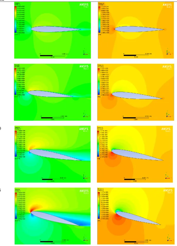
Table 1 illustrates distribution pressure and velocity at four different angles of attack, it can be noticed that, pressure distribution in top and bottom domain (compared to chord) is asymmetry at 0o angle of attack. In this
case, it is hard to rotate the blade of the marine turbine due to relative similar pressure distribution between top and bottom domain. In others of angles of attack, pressure distribution in the down domain always has the larger values than the case of 0o angle of attack. In addition, when angle of attack gets up, average of pressure also
increase respectively. It is easy to see that when angle of attack is not 0o, the blade of the marine turbine can rotate
conveniently thank for different pressure distribution among two domains.
(a)
(b)
Fig.4.Convergence graph of (a) Cl and (b) Cd
From velocity contour, it can be seen when the angle of attack is increased, maximum velocity is increased too. But high velocity is concentrated at spike of NACA shape. It means drop-pressure will be happened, and lead to turbulent flow at back of NACA shape.
other hand, shape of NACA HF-SX is not symmetric, because pressure in top domain is less than pressure at bottom domain, although other cases at 5o, 10o and 15o, difference between top domain and bottom domain is
noticed. The value of pressure at the lower domain is always higher than the value of pressure at higher domain. However, to determine the cases with highest ratio, it is must to get the numerical values at top and bottom surface of NACA shape. All parameters value and results are shown in the Table. 2.
Table 1. Distribution pressure and velocity at four different angles of attack
Angle attack
Pressure Distribution Velocity Distribution
0
5
10
Table2. Show value Cl, Cd, Max Pressure, Min Pressure, Min Velocity and ratio Cl/Cd
Angle of attack Cl Cd Max Pressure
(Pa) Min Pressure (Pa) Max Velocity (𝑚 𝑠⁄ ) Cl/Cd 0 1.053 0.01509 4440 -2140 3.487 69.78 5 1.5991 0.01868 4339 -7046 4.482 85.6 10 1.9364 0.02938 5177 -14200 4.804 65.9 15 1.958 0.08203 4460 -23970 5.693 23.86 5. VALIDATION OF CFD RESULTS
Fig. 5 shows relationship between Cl and angle of attack. The Cl is directly affected by angle of attack, at angle
0 degree Cl = 1.053 which is minimum value, at angle 5 degree Cl = 1.5991, at 10 degree is 1.9364 and at 15
degree Cl is 1.958. In general, the lift coefficient increases with the increase of angle of attack. In addition, the lift
coefficient is proportional to angle of attack where the trend of curve is reduced when angle of attack increases, which means that the rate of increasing of lift coefficient is decreased when angle of attack increase than the value of 15 o.
Based on lift coefficient curve of proposed model and experimental results of NACA HF-SX [35], the trend of two curves in Fig. 5 is relatively similar. Furthermore, the numerical results of Cl and Cd have been agreed with
experimental results at different angle of attack. In particular, at 15 degree in two models lift coefficients values
are about 2.
(a) (b) Fig.5. Cl for NACA HF-SX (a) proposed model; (b) experimental [adopted from 35]
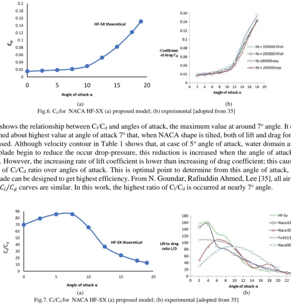
Fig. 6 shows relationship between Cd at different angles of attack. At angle 0 degree Cd = 0.01509 (i.e.
minimum value of Cd); at angle 5 degree Cd = 0.01868; at 10 degree is 0.02938 and at 15 degree is 0.08203.The
peak of the ratio Cl/ Cd is at around 7 o angle of attack from Fig. 8 bellow. Similar to the lift coefficient, the drag
coefficient also increases with angle of attack. In spite of this curve is non-linear, it is similar with lift coefficient curve, and it is covariates too, so the drag coefficient is proportional to angle of attack. Also, slope of curve is increased when angle of attack increases, because the speed of increasing of lift coefficient will be increased when angle of attack increases.
Based on drag coefficient curve of proposed model and experimental results of NACA HF-SX [35], the drag coefficients are proportional to angles of attack. The trend of proposed model and experimental results are relatively agreed. Moreover, magnitude of lift coefficient at angle of attack levels also nearly equal; e.g. at 15 degree in two models drag coefficients values are about 0.08.
1 1.2 1.4 1.6 1.8 2 2.2 2.4 0 5 10 15 20 Cl Angle of attack α HF-SX theoretical
(a) (b) Fig.6. Cd for NACA HF-SX (a) proposed model; (b) experimental [adopted from 35]
Fig. 7 shows the relationship between Cl/Cd and angles of attack, the maximum value at around 7o angle. It can
be explained about highest value at angle of attack 7o that, when NACA shape is tilted, both of lift and drag forces
are increased. Although velocity contour in Table 1 shows that, at case of 5o angle of attack, water domain after
spike of blade begin to reduce the occur drop-pressure, this reduction is increased when the angle of attack is increased. However, the increasing rate of lift coefficient is lower than increasing of drag coefficient; this cause a reduction of Cl/Cd ratio over angles of attack. This is optimal point to determine from this angle of attack, the
turbine blade can be designed to get highest efficiency. From N. Goundar, Rafiuddin Ahmed, Lee [35], all airfoil trends of 𝐶𝑙/𝐶𝑑 curves are similar. In this work, the highest ratio of Cl/Cd is occurred at nearly 7o angle.
(a) (b) Fig.7. Cl/Cd for NACA HF-SX (a) proposed model; (b) experimental [adopted from 35]
6. CONCLUSION
Based on the results of analysing the flow field around the aerofoil of turbine, the performance of marine turbine is directly affected by the angle of attack. This is clearly shown by the drag and lift coefficients, where Cd
and Cl coefficients increases with increasing the angle of attack. Hence, from Cl/Cd curve, the blades performance
reaches the peak at around 7o angle of attack.
In conclusion, at the zero degree of angle of attack, there is a relatively small lift force generated, and if it is desired to increase in the amount of lift force and the value of lift coefficient the angle of attack have to be increased. By doing that obviously amount of drag force and value of lift coefficient also increased, but the increment in drag coefficient is slightly lower than lift force. Also, from results of velocity contour, the location of cavitation phenomenon can be located and determined. The pressure contour shows location of the high stress on the material; hence it has to reinforce or may propose other materials. Finally, from all analysed results, the performance of marine turbines is directly affected by angle of attack. In the future, a 3-D study with these data can be coupled with structure analysis method, i.e. finite element analysis, to improve the marine current turbines efficiency. 0 0.02 0.04 0.06 0.08 0.1 0.12 0.14 0.16 0.18 0.2 0 5 10 15 20 Cd Angle of attack α HF-SX thoeretical 0 10 20 30 40 50 60 70 80 90 0 5 10 15 20 Cl /Cd Angle of attack α HF-SX thoeretical
REFERENCES
1. C.E. Morris, D.M. O’Doherty, A. Mason-Jones, T. O’Doherty, Evaluation of the swirl characteristics of a tidal stream turbine wake, International Journal of Marine Energy, 2016, 14, 198–214.
2. Elbatran AH, Yaakob OB, Ahmed YM, Shabara HM. Numerical study for the use of different nozzle shapes in microscale channels for producing clean energy. International Journal of Energy and Environmental Engineering. 2015, 6(2), 137-46.
3. A.S. Bahaj, A.F. Molland, J.R. Chaplin, W.M.J. Batten, Power and thrust measurements of marine current turbines under various hydrodynamic flow conditions in a cavitation tunnel and a towing tank, Renewable Energy, 2007, 32(3), 407-426.
4. B Y Xiao, L J Zhou, Y X Xiao and Z W Wang, The prediction of the hydrodynamic performance of marine current turbines, Materials Science and Engineering, 2013, 52.
5. Van der Plas, The effect of platform motions on turbine performance: A study on the hydrodynamics of marine current turbines on the floating tidal energy converter BlueTEC, Master Thesis, University of Malta , 2014.
6. Mayurkumar kevadiya, Hemish A. Vaidya, 2d analysis of NACA 4412 airfoil, International Journal of Innovative Research in Science, 2013, 2(5).
7. Elbatran AH, Yaakob O, Ahmed Y, Abdallah F. Augmented, Diffuser for Horizontal Axis Marine Current Turbine. International Journal of Power Electronics and Drive Systems. 2016, 7(1), 235.
8. S. Dajani, M. Shehadeh, N. Hart, D. Cheshire, Aspects of Tidal Power Resources in Egypt, International conference on Recent Advances in Energy Systems (RAEPS-12), Alexandria, Egypt, 2012, 17-20.
9. Ahmed S. Shehata, Khalid M. Saqr, Qing Xiao, Mohamed F. Shehadeh, Xianghong Ma, Alexander Day, Performance analysis of wells turbine blades using the entropy generation minimization method, renewable energy, 2016, 86C, 1123-1133.
10. Long Chen, Wei-Haur Lam, Slipstream between marine current turbine and seabed, Energy, 2014, 68, 801–810.
11. Tiago A. de Jesus Henriques, Terry S. Hedges, Ieuan Owen, Robert J. Poole, The influence of blade pitch angle on the performance of a model horizontal axis tidal stream turbine operating under wave – current interaction, Energy, 2016, 1, 166– 175.
12. Rajesh Bhaskaran, Lance Collins, Introduction to CFD Basics, Cornell University, 2012, USA.
13. Iham F. Zidane, Khalid M. Saqr, Greg Swadener, and Mohamed F. Shehadeh, CFD Study Of Dusty Air Flow Over NACA 63415 Airfoil For Wind Turbine Applications, 9th International Meeting on Advances in Thermo fluids (IMAT-2017), UTM, Johor, Malaysia.
14. Shehadeh M, Sharara A, Khamis M, El-Gamal H., A Study of Pipeline Leakage pattern Using CFD. Canadian Journal on Mechanical Sciences & Engineering, 2012, 3(3), 98-101.
15. Shahata AI, Youssef MT, Saqr K, Shehadeh M., CFD Investigation of Slurry Seawater Flow Effect in Steel Elbows. International journal of engineering research and technology, 3(1), 2014, 364-370.
16. Mario Oertel, Environmental Hydraulic Simulation, Lecture material, Lübeck University of Applied Science, Germany.
17. Elbatran AH., DES of the turbulent flow around a circular cylinder of finite height. Journal of Naval Architecture and Marine Engineering. 2016, 29, 13(2), 179-88.
18. Iham F. Zidane, Khalid M. Saqr, Greg Swadener, Xianghong Ma and Mohamed F. Shehadeh, On the role of surface roughness in the aerodynamic performance and energy conversion of horizontal wind turbine blades: a review, International Journal of Energy Research 2016, 40(15), 2054-2077.
19. T.S.D.Karthik, Turbulence Models and Their Applications, 10th Indo German Winter Academy, 2011, Germany.
20. Elbatran AH, Yaakob OB, Ahmed YM, Jalal MR., Novel approach of bidirectional diffuser-augmented channels system for enhancing hydrokinetic power generation in channels. Renewable Energy. 2015, 30, 83:809-19.
21. Karna S. Patel, Saumil B. Patel, Utsav B. Patel, Ankit P. Ahuja, CFD Analysis of an Aerofoil, International Journal of Engineering Research, 2014, 3(3), 154-158.
22. Ivaylo Nedyalkov, Martin Wosnik, Performance of Bidirectional Blades for Tidal Current Turbine, Proceedings of the ASME 2014 4th Joint US-European Fluids Engineering Division Summer Meeting, 2014, USA.
23. R. Noruzi, M. Vahidzadeh, A. Riasi, Design, analysis and predicting hydrokinetic performance of horizontal marine current axial turbine by consideration of turbine installation depth, Ocean Engineering, 2015, 789-798.
24. Jai N. Goundar, Numerical and experimental studies on hydrofoils for marine current turbines, Renewable Energy, 2011, 42, 173-179.
25. Ceri Morris, Influence of Solidity on the Performance, Swirl Characteristics, Wake Recovery and Blade Deflection of a Horizontal Axis Tidal Turbine, Ph.D. Thesis, Cardiff University, 2014, UK.
26. Douglas S. Cairns, Airfoils, Wings, and Other Aerodynamic Shapes – a mini course on aerodynamics, Lecture Material, Montana State University, USA.
27. http://airfoiltools.com, Nov 2016
28. Sachin Srivastava, C.V.N Aditya, Analysis of NACA 2412 Airfoil for UAV Based on High-Lift Devices, International Journal of Engineering Applied Sciences and Technology, 2016, 1(6), 13-16.
29. Christopher J. Roy, Strategies for Driving Mesh Adaptation in CFD, 47th AIAA Aerospace Sciences Meeting including The New Horizons Forum and Aerospace Exposition, 2009, Florida, USA.
30. ANSYS Fluent UDF Manual, 275 Technology Drive Canonsburg, USA.
31. http://www.livescience.com/47188-ocean-turbines-renewable-energy.html, Nov 2017.
32. William Gracey, Measurement of static pressure on aircraft, NACA Technical Report, National Advisory Committee for Aeronautics Collection, 1958, USA.
33. Weltner, Klaus; Ingelman-Sundberg, Martin, Misinterpretations of Bernoulli's Law, University of Frankfurt, 2009, Germany.
34. http://marinebio.org/oceans/temperature/, Nov 2016.
35. Jai N. Goundar, M. Rafiuddin Ahmed , Young-Ho Lee, Numerical and experimental studies on hydrofoils for marine current turbines, Renewable Energy, 2012, 42, 173-179.