Video Object Counting in Unconstrained Environments Using Density-Based Clustering

(1)

Unconstrained Environments

Using Density-Based Clustering

by

Onalenna Junior Makhura

A thesis submitted for the degree of PhD

Department of Computer Science and Electronic Engineering University of Essex

(2)

(3)

In this thesis, we present a video object counting approach using multiple local feature matching. We explain the development of a dataset with which to test our approach. Our dataset uses a new approach which we designed to extract object ground truth. We also provide a comparison of common single object trackers. We develop a multi-object tracker named Learn-Select-Track and use it to track the colours of multi-objects of interest to filter out false positive object localisations.

We discuss the implementation of the HDBSCAN algorithm which we use in our novel approach for matching multiple local feature descriptors. We show that the detected clusters provide very good matches for the features and demonstrate our approach to cluster analysis and validation. We develop a simple yet efficient way of learning the features of the object of interest which is independent of the number of objects in the frame.

We also develop a computationally simple way of detecting the other objects in the frame by using a combination of the detected clusters, the features of the object of interest and vector algebra. Our approach is capable of detecting partially visible and occluded objects as well. We present three ways of extracting object count estimations from videos and provide empirical evidence to show that our approach can be used in a wide variety of scenarios.

(4)

(5)

“The most valuable gift you have to offer is yourself - The

Go-Giver, Burg and Mann"

(6)

(7)

I, Onalenna Junior Makhura, declare that this thesis titled, ‘Video Object Count-ing in Unconstrained Environments UsCount-ing Density-Based ClusterCount-ing’ and the work presented in it are my own. I confirm that:

This work was done wholly or mainly while in candidature for a research degree at this University.

Where any part of this thesis has previously been submitted for a degree or any other qualification at this University or any other institution, this has been clearly stated.

Where I have consulted the published work of others, this is always clearly attributed.

Where I have quoted from the work of others, the source is always given. With the exception of such quotations, this thesis is entirely my own work.

I have acknowledged all main sources of help.

Where the thesis is based on work done by myself jointly with others, I have made clear exactly what was done by others and what I have contributed myself.

Signed:

(8)

(9)

First, I would like to acknowledge my supervisor Dr. John Woods. He has been a rock steady guide for me in this journey. From the moment I contacted him to be my supervisor, he has been kind and supportive. He offered me great advice and encouragement which I will forever be grateful for. I pray that he may forever be such a wonderful supervisor for many more aspiring PhD student like me.

I would also like to acknowledge my family. My mother, Leah Masilo, has always been a symbol of calm strength. She has been an example of how to weather the difficulties without losing who you are. Her faith in me has never wavered, which has greatly influenced me to give my best. My son, Bonno Michael Mokgobi has always been a beacon of hope and direction in my life. He always helps me remember what is truly important in my life.

I would be forgetful if I do not acknowledge my friends, who have always encouraged and believed in me. Obakeng and Lebogang, who have been my friends for more than 15 years. Without them, my affairs at home would not have been taken care of while I pursue my PhD. Dr. Thabiso Maupong has been an inspiration for me. I am so glad that he was 2 years ahead of me which served as a perfect template of how to approach my PhD studies. His guidance and advice were truly amazing. To Kabo, Kagiso, Ella, Khana and Wada, I hope to repay your kindness one day. You guys are awesome.

My sponsor, the University of Botswana has literally given me my dream of pursuing PhD and a career in academics. Through the Training Department, my studies have been a smooth road. Even though I was a pain at times, the staff handled things brilliantly. Special recognition to Neo Seroke who has handled my interactions with them with grace and always with a smile on her face.

Last, and most importantly, I would like to appreciate God for all the blessings I mentioned above and many more. The presence of all these wonderful people in my life could only have been by His grace. He has always been a voice in my heart guiding me to be where I am today. I will forever be grateful and thankful to Him.

(10)

(11)

List of Figures x

List of Tables xv

List of Listings xix

Glossary xx

1 Introduction 1

1.1 Review of Object Counting Approaches . . . 3

1.1.1 Counting By Object Density Estimation . . . 3

1.1.2 Counting By Object Detection. . . 5

1.1.3 Counting By Trajectory Clustering . . . 7

1.2 Proposed Approach to Object Counting . . . 8

1.3 Thesis Outline . . . 14

2 Development of a Video Object Counting Dataset 16 2.1 Object Counting Dataset Challenges . . . 19

2.1.1 Inter Object Occlusion and Partial Visibility . . . 19

2.1.2 High Object Density . . . 20

2.1.3 Scale . . . 21

(12)

3.4.2 DBSCAN . . . 49

3.4.3 Hierarchical DBSCAN . . . 51

3.4.4 HDBSCAN Implementation . . . 53

3.4.5 Cluster Analysis and Validation . . . 54

3.5 Summary . . . 59

4 Multiple Local Feature Instance Detection 61 4.1 Multiple Features as Density-Based Clusters . . . 62

4.1.1 Lowe’s Ratio in Clusters . . . 66

4.1.2 Cluster Feature Similarity . . . 68

4.2 Varying minPts . . . 78

(13)

4.4 Rotational Invariance . . . 82

4.5 Summary . . . 86

5 Colour Model Tracking 87 5.1 Learn-Select-Track . . . 88

5.1.1 Training . . . 88

5.1.2 Track and Update. . . 91

5.2 Colour Model Training and Tracking Results . . . 92

5.2.1 Colour Model Training . . . 92

5.2.2 Frame by Frame Colour Tracking . . . 100

5.2.3 Training and Tracking Times . . . 103

5.3 Summary . . . 106

6 Object Locations and Count Estimations 108 6.1 Object of Interest Feature Learning and Tracking . . . 109

6.2 Object Localisation . . . 112

6.2.1 Cluster Objects Localisation . . . 112

6.2.2 Scale Challenges . . . 114

6.2.3 Rotational Invariance . . . 119

6.2.4 Occlusion and Partial Visibility . . . 120

6.2.5 Complex Background . . . 121

6.3 Frame Count Estimation . . . 126

6.4 Iterative Cluster Daisy-Chain . . . 128

6.5 False Positive Locations Detection and Elimination . . . 133

6.5.1 Frame Object Count using Colour Model Clusters . . . 133

6.5.2 Frame Descriptor Locations Combined with Colour Model Lo-cations . . . 136

6.6 Summary . . . 141

7 Video Object Count Estimations 143 7.1 Video Count Estimations . . . 144

7.1.1 Frame Descriptors . . . 146

(14)

B Best Counting Estimation Results 186 B.1 VOC-18-BD-1 . . . 187 B.2 VOC-18-BD-2 . . . 188 B.3 VOC-18-BD-3 . . . 189 B.4 VOC-18-BD-4 . . . 190 B.5 VOC-18-BD-5 . . . 191 B.6 VOC-18-BD-6 . . . 192 B.7 VOC-18-BD-7 . . . 193 B.8 VOC-18-BD-8 . . . 194 B.9 VOC-18-BD-9 . . . 195 B.10 VOC-18-BD-10 . . . 196 B.11 VOC-18-BD-11 . . . 197 B.12 VOC-18-BD-12 . . . 198 B.13 VOC-18-BD-13 . . . 199 B.14 VOC-18-BD-15 . . . 200 B.15 VOC-18-BD-17 . . . 201 B.16 VOC-18-BD-18 . . . 202 B.17 VOC-18-BD-19 . . . 203 B.18 VOC-18-BD-20 . . . 204 B.19 VOC-18-BL-1 . . . 205

(15)

B.20 VOC-18-BL-2 . . . 206

B.21 VOC-18-BL-3 . . . 207

(16)

List of Figures

1.1 Concept of object counting for this thesis. On a frame-by-frame basis, the approach takes as input an ROI identifying one of the objects, and the SURF features from the frame and produces an estimation of the number of object in the frame by locating each instance of the object. 10

2.2 The occlusion challenge as seen invoc-18-bd-1 video. . . 20

2.3 The high object density challenge from voc-18-bl-1 video. . . 21

2.4 The scale challenge as seen invoc-18-bd-14 video with the binary image representation of the ground truth. . . 22

2.5 The vanishing point challenge in voc-18-bd-18 video with the binary image representation of the ground truth.. . . 23

2.6 Examples of complex background challenges in our dataset. . . 24

2.7 A frame and its binary version for video file voc-18-bl-4. . . 26

2.8 The structure of the VOC-18 dataset as it appears on github. . . 28

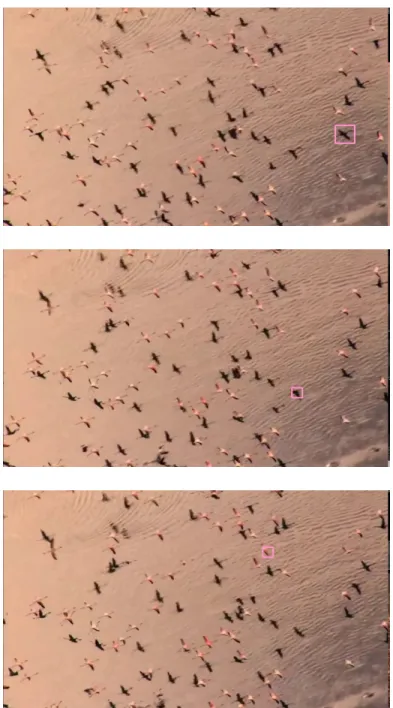
3.1 The detector “jumping” problem in TLD withvoc-18-bd-3 video. . . 39

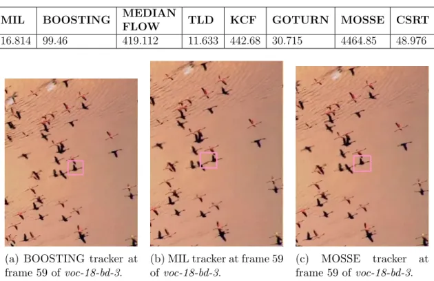
3.2 Comparisons of BOOSTING, MIL and MOSSE onvoc-18-bd-3 video. 41 3.3 Comparisons of BOOSTING, MIL and MOSSE onvoc-18-bd-11 video. 42 3.4 The susceptibility of CSRT to appearance variations. . . 42

3.5 Oriented quadratic grid with 4x4 square sub-regions is laid over the interest point and the P dx, P dy, P |dx|, P |dy| . . . 46

(17)

3.6 Parta shows the concept of border points and core points in a cluster. Part b shows the ε-neighbourhood of both p and q. In a cluster, the points are such that the ε-neighbourhood of core points contain the number of points less than or equal to the value of minPts. . . 50

3.7 Part a illustrates how p is density-reachable from q while the reverse is not true. Partb shows how point p is density connected to point q. 50

4.1 Differences in the number of features in LODVs, MODVs and HODVs. 65

4.2 Visualisation of some of the clusters from Table 4.4. . . 69

4.3 Visualisation of some of the clusters from Table 4.5. . . 75

4.4 Visualisation of some of the clusters from the first frame ofvoc-18-bd-1

HODV.. . . 76

4.5 Visualisation of some of the noise clusters between frames 1 and 2 of

voc-18-bd-6 LODV. . . 77

4.6 The splitting of cluster 12 from minP ts = 3 into 5 clusters with

minP ts= 2. . . 81

4.7 The same cluster discovered in frame 1 ofvoc-18-bd-20 withminP ts = [2,3]. . . 82

4.8 Rotational invariance in SURF. . . 83

4.9 Results of augmenting descriptors with angles invoc-18-bd-15 frame 17. 85

5.1 Training, and tracking the colour model of voc-18-bd-1. . . 95

5.4 Options for colour selectionvoc-18-bd-10 video. With selectedminP ts= 11, 3 non-noise clusters were detected and offered as choices for the colour model. . . 99

5.5 The tracker results for voc-18-bd-12 video showing successful colour model tracking from the first to the last frame.. . . 100

5.6 The problem posed by object colours that are similar to the back-ground colours. . . 101

5.7 The graph of number of points vs time for learning the object colour model on the first frame. . . 105

(18)

LIST OF FIGURES

5.8 The graph of average number of point per frame vs the tracking duration.105

6.1 Re-initialisation of the tracker when the target breaches the ten pixel

barrier.. . . 110

6.2 The effect of scale in re-initialising the tracker when the object moves off the frame. . . 111

6.3 Comparison of raw shifting and shifting with template matching.. . . 114

6.4 Locations of birds in voc-18-bd-1 for different clusters. The first sub-figure shows the false positive locations while the other two show ac-curate localisations. . . 115

6.5 Cluster features drawn to show scale invariance of the SURF features. 116 6.6 Evidence of feature scale not representing object size. . . 117

6.7 Failure of localisation algorithm to find the other objects due to ex-treme scale challenges in voc-18-bd-16. . . 118

6.8 Comparison of object localisation with and without rotational consid-eration. . . 122

6.9 Susceptibility of the localisation algorithm to partial occlusion. . . 123

6.10 Susceptibility of the localisation algorithm to partial visibility. . . 124

6.11 False positives from background features. . . 125

6.12 Final object localisations and multiple clusters identifying the same objects. . . 126

6.13 Example of noisy clusters in creating false positive locations. In these images, the noise can be noticed because some features are on the object while others are on the background where the colours are no-ticeably different. . . 127

6.14 Iterative cluster daisy-chaining to discover clusters that do not inter-sect with the initial ROI in order to reduce false negatives. . . 131

6.15 Iterative cluster daisy-chaining introducing false positives. . . 132

6.16 Detecting clusters in the colour model features in frame 1 ofvoc-18-bd-12.134 6.17 The clusters from the frame descriptors. . . 138

6.18 Comparison between frame descriptor localisation and colour model localisation. In this figure we used varying minPts and no rotation or cluster over-segmentation. . . 139

(19)

6.19 Combining the locations detected using frame descriptors and colour

model descriptors to get rid of the false positive locations. . . 140

7.1 The presence of SURF features dictate how many objects our approach can detect. Invoc-18-bd-14 andvoc-18-bd-16, the tracker even lost the initial object due to localisation failure. . . 146

7.2 An example of how our approach can fail to detect any objects due to ROI features being labelled as noise. . . 148

7.3 Difference between colour model and frame descriptor clustering re-sults. In both results, augmented descriptor clustering was done with minP ts= 2 and no cluster daisy chaining. . . 150

7.4 Stabilisation of HODV results as more iterations are used. . . 158

B.1 Combined object localisations for the first 4 frames of voc-18-bd-1. . . 187

B.2 Combined object localisations for the first 4 frames of voc-18-bd-2. . . 188

B.3 Object localisations for the first 4 frames of voc-18-bd-3. . . 189

B.10 Combined object localisations for the first 4 frames of voc-18-bd-10. . 196

B.12 Combined object localisations for the first 4 frames of voc-18-bd-12. . 198

B.19 Object localisations for the first 4 frames of voc-18-bl-1. . . 205

(20)

LIST OF FIGURES

B.21 Object localisations for the first 4 frames of voc-18-bl-3. . . 207

(21)

2.1 Low Object Density Videos . . . 28

2.2 Medium Object Density Videos . . . 28

2.3 High Object Density Videos . . . 29

2.4 Challenges posed by each video. . . 30

3.1 Average FPS of the OpenCV SOTs using the voc-18-bd-1 video. . . . 41

4.1 The number of SURF features detected for LODVs. . . 63

4.2 The number of SURF features detected for MODVs.. . . 63

4.3 The number of SURF features detected for HODVs. . . 64

4.4 This table shows the closest features to two features from cluster 100 in frame 1 of voc-18-bd-1. The cluster had 4 features. . . 67

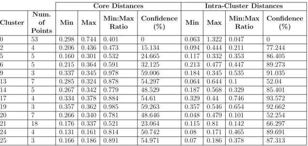
4.5 Cluster data from voc-18-bd-20 frame 4 with minP ts= 4. . . 71

4.6 The first 8 frames of voc-18-bd-6 showing the variations in number of clusters and the validities from frame to frame.. . . 72

4.7 The clusters detected in frame 1 ofvoc-18-bd-6. The clustering results had validity = 0. . . 72

4.8 The clustering validity statistics for LODVs forminP ts = 3. . . 73

4.9 The clustering validity statistics for MODVs for minP ts= 3.. . . 74

4.10 The clustering validity statistics for HODVs for minP ts= 3. . . 74

4.11 The clustering validity statistics for LODVs with varyingminPts values. 79

(22)

LIST OF TABLES

4.13 The clustering validity statistics for HODVs for varying minP ts values. 79

4.14 The effects of varying minPts in frames 17 and 18 in voc-18-bl2. . . . 80

5.1 The training results with VOC-18 dataset. The ‘Points’ column shows the number of colour points detected in the first frame and ‘Time’ column shows the amount of time it took to analyse the colours by the training algorithm. . . 93

5.2 The results of tracking the colours based on the selected colours. . . . 102

5.3 The table showing the videos where the tracker lost the model instantly.102

5.4 The average number of features being tracked per frame and the aver-age time taken to process each frame arranged in ascending order. . . 104

6.1 Selected clusters in frame 10 of vo-18-bd-1. . . 114

6.2 Distance values of the selected clusters in voc-18-bd-16 frame 23 with

minP ts= 3. . . 118

6.3 Distance values of the selected clusters in voc-18-bd-16 frame 23 with

minP ts= 2. . . 119

6.4 Object count estimations using various iteration values forminP ts= 2 and 3 on frame 1 of voc-18-bd1. . . 129

6.5 The clusters detected . . . 134

7.1 LODV counting estimations using the frame descriptors. . . 147

7.2 MODV counting estimations using the frame descriptors. . . 147

7.3 HODV counting estimations using the frame descriptors. . . 148

7.4 LODV counting estimations using the colour model descriptors. . . . 150

7.5 Colour model clustering estimation results forvoc-18-bd-10 whose ground truth is min = 9, max = 18, µ = 13.82, σ = 2.96 showing the close similarities between the results for various parameters. . . 152

7.6 MODV counting estimations using the colour model descriptors. . . . 152

7.7 HODV counting estimations using the colour model descriptors. . . . 152

7.8 LODVs counting estimations using the combined frame and colour model descriptor locations. . . 153

7.9 MODVs counting estimations using the combined frame and colour model descriptor locations. . . 154

(23)

7.10 HODVs counting estimations using the combined frame and colour model descriptor locations. . . 154

7.11 LODV best counting estimations. . . 156

7.12 MODV best counting estimations. . . 156

7.13 HODV best counting estimations. . . 157

B.1 Count estimation for voc-18-bd-1 using combined frame and colour model descriptor results and parameters minP ts = 3, I = 1, O =

Y, R=N. . . 187

N, R=Y. . . 188

B.3 Count estimation for voc-18-bd-3 using frame descriptors and param-eters minP ts= 2, I = 4, O =Y, R =Y. . . 189

B.4 Count estimation for voc-18-bd-4 using frame descriptors and param-eters minP ts= 2, I = 0, O =Y, R =N.. . . 190

B.5 Count estimation for voc-18-bd-5 using colour model descriptors and parameters minP ts= 2, I = 0, O=Y, R =Y. . . 191

Y, R=Y. . . 196

(24)

LIST OF TABLES

N, R=N. . . 198

Y, R=Y. . . 204

B.19 Count estimation for voc-18-bl-1 using frame descriptors and parame-ters minP ts= 2, I = 5, O =Y, R =Y. . . 205

Y, R=Y. . . 206

B.21 Count estimation for voc-18-bl-1 using frame descriptors and param-eters minP ts = 2, I = 2, O =Y, R =Y for the first 26 frames where the initial object was successfully tracked. . . 207

B.22 Count estimation for voc-18-bl-1 using frame descriptors and parame-ters minP ts= 2, I = 2, O =Y, R =Y. . . 208

(25)

A.1 Function for encoding and decoding the indices into the optimised distance array. . . 182

A.2 Function for retrieving the distance values from the optimised distance array.. . . 182

A.3 Getting the core distances from the optimised array. . . 183

A.4 Function for calculating euclidean distances given an array of vectors. The distances are stored in an array optimised for memory. The func-tion uses OpenMP to parallelise the ditance calculafunc-tions. . . 183

A.5 Extracting and saving video frames . . . 184

A.6 Extracting ground truth from binary images . . . 184

A.7 Creating an LMDB database for the ground truth . . . 185

(26)

Glossary

ANN - Artificial Neural Network designed for classification tasks by mimicking the way the brain learns patterns in data..

CNN - Convolutional Neural Network designed for image processing. Useful for object recognition.

DBSCAN - Density based clustering algorithm for finding clusters in data..

FLANN - Fast Library for Approximating Nearest Neighbours.

HDBSCAN - Hierarchical DBSCAN designed to have the ability to find varying density clusters by finding all possible DBSCAN solutions..

HODV - High Object Density Videos are videos where object count are more than 50. These videos provide the highest chance for object occlusions and false positive object locations..

LODV - Low Object Density Videos have object count less than 10. These videos often have very detailed objects that are close to the camera recording the video. They are often subject to over clustering of the features leading to some objects being identified multiple times..

(27)

MODV - Moderate Object Density Videos have object count greater than 10 but less than 50. These videos have a less chance of object occlusions. The object count estimations are subject ot whichever end of the scale the ground truth count is..

OpenCV - A suite of open source computer vision libraries. The library is imple-mented in C++ with python, java and matlab bindings. For this thesis, this library was used to handle video file frame extraction, object tracking and local feature extraction..

SIFT - Scale Invariant Feature Transform.

(28)

Publications

1. O. Makhura and J. Woods, “Multiple feature instance detection with density based clustering,” in 2018 IEEE International Conference on Consumer Elec-tronics (ICCE) (2018 ICCE), (Las Vegas, USA), Jan. 2018.

2. O. J. Makhura and J. C. Woods, “Learn-select-track: An approach to multi-object tracking,” Signal Processing: Image Communication, vol. 74, pp. 153 – 161, 2019.

3. O. Makhura and J. Woods, “Video object counting dataset,” in 2019 IEEE Conference on Multimedia Information Processing and Retrieval (MIPR), (San Jose, USA), pp. 1 – 4, Mar 2019.

(29)

Chapter

1

Introduction

The ability to quantify objects is one of the ways of extracting semantic informa-tion about a scene. Therefore, object counting using computer vision techniques is a highly active and evolving research field. The algorithms developed have been ap-plied in a wide variety of problems across the whole spectrum of human lives. For example, in large scale industries where thousands of products have to be counted, object counting algorithms are critical to industrial efficiency and profitability. In such industrial applications, computer vision based object counting can benefit from the controllability of the environment. The counting environment background and lighting are some of the factors that can be tightly controlled. The objects to be counted are often inanimate, as such, their size, colour and texture are static, allow-ing for countallow-ing algorithms that are tailor made for specific environments.

In such environments, it is common to see algorithms that rely on background sub-traction in use. In those situations, since the background is known and static, its value can be removed from the images or video frames, and whatever colour is left can be considered to belong to the objects of interest. Histogram analysis can be accurately used in such environments since the size and colour of the objects are known. Other common algorithms include shape detectors, blob detectors and contour extraction algorithms.

(30)

CHAPTER 1. INTRODUCTION

Object counting is also being employed by animal conservation societies like Birdlife International [1] and Convention on International Trade on Endangered Species of Wild Fauna and Flora (CITES) [2]. Unlike the industrial environments, the animals are often in remote areas that are not easily accessible and the environment is even less controlled. Technological advances in areas such as satellite imagery and unmanned aerial vehicles (UAV) are giving researchers and conservationists access to such hard to reach places. A good example of use of such technologies can be found in [3], where the authors demonstrated using super-high resolution NASA satellite images to count albatrosses in the remote region of Chatham Islands.

In Botswana, Birdlife Botswana [4] published a guideline for monitoring bird popu-lation [5]. The process requires people to walk around in a set pattern and recording the count estimations of the birds they see. The obvious downsides to this approach is the cost in human capital and the inaccuracy of relying on humans to count birds in motion. Other factors such as fatigue and object density can affect the reliability of human object counting [6,7]. The document even notes the need for “scientifically sound low-tech monitoring methodology” while noting the need for their approach to be implemented by “as many participants as possible”. With vultures across Africa facing extinction [8,9], Birdlife Botswana also has signs across the country asking the public for information on vulture sightings.

The increase in accessibility of low cost but high quality imaging devices such as UAVs and smartphones can provide powerful tools to address the challenges highlighted above. The bird population monitors can use these devices to record the videos of birds for analysis later instead of just estimating the numbers based on what they are seeing then. With algorithms such as the one detailed in this thesis, the videos can be analysed to obtain more accurate and consistent count estimation. Even the public can use their smartphones to record the vulture sightings and send the videos to Birdlife Botswana for analysis.

The other problem in wildlife population monitoring is the widely diverse environ-ments where the animals can be found. In order to be successful, object counting algorithms would have to be either designed for specific environments e.g. water, sky, clouds, forest etc., or they would need an in-built capability to adapt to these

(31)

ever changing parameters. The approach described in this thesis focusses on the latter which means the algorithm can be deployed in different environments without any changes to how it processes the videos. Usually algorithms designed for non-constrained environments require a lot of time and data to train them. With infinite classes of objects that one may be interested in counting, the problem becomes more than just counting, the problem extends to counting any object.

In this thesis, the focus is on object counting for videos taken in unconstrained environments. The idea behind this research is to take a random video containing multiple instances of an object of interest, and using image and video processing computer vision algorithms, to identify all the object instances and give a count of the objects in the video frame. With consumer generated video data, the environments under which the object count must be extracted is unconstrained which provides a challenge for algorithms to be generic yet accurate. The scope of this thesis does not include aggregating the number of objects in the video, but rather, the number of objects in each video frame.

1.1

Review of Object Counting Approaches

In this section we review some of the recent object counting literature. In this the-sis, we recognise three groups of object counting approaches. We first discuss the density estimation approaches which work by using image density maps and local feature mapping to estimate number of objects. Then we review object counting using object detection which aim to detect and localise objects of interest in images. Finally, we discuss counting by trajectory clustering approaches which are designed for video object counting through object motion detection. We discuss the findings and the shortcomings of these approaches which work by detecting object movements in videos.

1.1.1

Counting By Object Density Estimation

Density estimation based counting methods estimate a real valued density function of pixels in a given image by mapping local features of the image to its density

(32)

CHAPTER 1. INTRODUCTION

map. These methods often require a set of manually labelled training images where they generate the ground truth density map, then extract local features and finally apply a regression model to learn the mapping between the local features and their corresponding density maps. The regression model is then used to estimate the density map of any image and the object count estimation is extracted by calculating the integral of the density map.

Density estimation based methods such as the one outlined in [10], tend to degrade in performance when new objects and scenes are encountered. In [11], the authors address this problem by proposing a manifold based density estimation counting method. Their approach is based on an assumption that the neighbouring image patches are more likely to share similar density patches, hence, images of objects share information as their density maps regarding the local geometries. As such the counting problem is converted into the problem of characterising the local geometry of a given image patch which makes their approach robust against features used and image resolution.

For this method, [11], the training requires annotated images and their ground truth density maps. The method then extracts image patches and their counterpart den-sity patches. These are used in a feature engineering stage to create a hierarchical clustering tree structure using K-Means algorithm. The tree structure is then used to estimate the density map for each image patch. The object count can then be extracted by an integral of the density map. This form of training is a weakness to this approach as the annotation and ground truth density map generation means that the learning has to be done offline. The approach has been tested on cells [10], bees, fishes, birds [12] and pedestrian [13–15] datasets.

Convolutional neural networks (CNN), which are a type of artificial neural networks (ANNs) designed with image processing in mind, are also a big part of object recog-nition and classification and have proven in recent years to have state of the art per-formances. CNNs work by using artificial neurons to learn weights that are needed to recognise objects in the training dataset. They have been used with great success in challenges such as the ImageNet LSVRC-2010 challenge where the design outlined in [16] successfully deployed aCNNachieved top-1 and top-5 error rates of 37.5% and

(33)

17.0% on a test data comprised of high resolution images. The accuracy of CNNs does not only rely on the dataset, they also rely on the design of the neural networks itself.

In [17], an adaptive Counting Convolutional Neural Network (A-CCNN) is proposed which has the ability to handle large scale variations in people sizes and the facility to generate local density maps within a crowd scene. In the paper, the authors do not try to use different CCNN architectures [18], instead, they only try to select the most effective hyper parameters to generate the CNN model. The approach uses as inputs, an image divided into 16 part and head sizes from different parts of the image detected using tiny-face detection [19]. The image patches are then fed to the appropriate CCNN model with a proper hyper parameter by using Fuzzy Inference System. The CCNN model then produces density maps for each image section which are merged to obtain final density map. The authors trained and tested their approach on the UCSD dataset [18], UCF-CC Dataset [13] and the Sydney Train Footage dataset.

1.1.2

Counting By Object Detection

Object recognition/detection is the identification of the presence of a “known object”. With a near infinite number of objects, the main challenge is how to best describe what any particular object looks like in such a manner that a computer can then be able to recognise it in any context. In order to define a particular object, there is need to break down the object into a set of features that together can be used to identify an occurrence of the object. The features can then be matched in target images and frames to locate the objects of interest. The total number of object locations identified therefore represent the number of objects detected.

Investigations into fish population estimation and species classification is addressed in [20]. The authors use background subtraction to find the fish and Zernike moments to classify the species. In [21] a probabilistic approach is proposed where multiple object instances are detected using Hough Transform. The authors show how to detect instances without dealing with the problem of multiple peak identification in Hough images and without invoking non maximum suppression heuristics. Their approach, instead, detects multiple object instances using maximum-a-posteriori in

(34)

CHAPTER 1. INTRODUCTION

the probabilistic model which contrasts the heuristic peak location and non-maximum suppression used in traditional Hough Transform.

In [22], a Density-based Clustering of Applications with Noise (DBSCAN) [23] is applied to Speeded-Up Robust Features (SURF) [24] in order to match a template to multiple inventory items. The approach extracts SURF features from both the prototype and the scene. Then DBSCAN is applied to the prototype features before applying feature mapping of the detected clusters to SURF points from the scene image. Sum of Squared Difference (SSD) and Nearest Neighbous Ratio (NNR) are used as matching factors.

DBSCAN is applied again to the scene features that have been matched to the tem-plate clusters and box information is extracted from the resulting clusters. Each of the clusters represents an instance of the prototype. Since there are multiple features within each cluster, there will be multiple boxes per instance. Box fixing is achieved by applying DBSCAN to the centroid locations to find the final box polygon. The approach uses hyper parameter tuning to determine the best values for minPts and . This approach is designed for handling images of inanimate inventory objects. As such, it is not tested on videos or and living objects. The paper also relies on the prototype and scene objects having enough features to form clusters.

CNNs and other deep learning approaches have two setbacks; dataset requirements and training requirements. These approaches require a lot of training data, time and computation. Therefore, they are not suitable for use in real-time to handle new object types. The datasets often have to be split into training, testing and validations subsets [25]. These datasets have to be prepared beforehand often through annotations which takes a lot of time and effort. It also limits their use in object counting to the learned objects.

The authors of [26] offer an approach towards generic object counting which aims to minimise the problems encountered when using CNNs. Their approach uses a fully convolutional network architecture where the input is an image and a hierarchy of image divisions. While there is an extra need to divide the image into localised divi-sions and hierarchies, the approach reduces the need for annotating training images

(35)

by global-image counts instead. They test their approach on MS-COCO [27], Pascal-VOC2007 [28] and CARPK [25] datasets. As a generic object counter, the authors did not eliminate the need for offline training and dataset preparation.

1.1.3

Counting By Trajectory Clustering

Movement of objects in a video has also been used for object counting. In [29], an algorithm for counting crowded moving objects by clustering a rich set of extended tracked features without requiring background subtraction is presented. The ap-proach uses a highly parallelised KLT tracker to populate the spatio-temporal volume with a large set of feature trajectories. Normally, the feature trajectories would be fragmented and noisy, hence, a conditioning algorithm is used to smooth and extend raw feature trajectories. The conditioned trajectories are clustered using agglomera-tive clustering into candidate objects using a local rigidity constrained learned from a small set of training frames. The authors note that the training frames have to be prepared beforehand by labelling them only with the ground truth count. This prohibits their algorithm from working with a completely new object.

In [30], an algorithm of counting people (pedestrians) using trajectory clustering is proposed. The authors address the fragmentation and noise problems in trajectories by applying a combination of linear transformations, i.e. independent component analysis (ICA) plus rotation. The approach explores different sets of data repre-sentations and distance/similarity measures. The data reprerepre-sentations are ICA, time series and maximum of cross-correlation (MSS). ICA is used with Euclidean distance, time series with longest common subsequence (LCSS) and MSS with Hausdorff dis-tance.

Their approach in [30] is multi-layered with three levels using agglomerative clus-tering to avoid having a priori knowledge of how many pedestrians are in the video. The first two layers are basically pre-processing levels where the first level is a length-based clustering in which trajectories of similar lengths are grouped together. The second level is spatial clustering where they acknowledge that different individuals enter the video frame at different locations, unless two or more individuals are walk-ing together. The actual countwalk-ing happens in level three where the discrimination

(36)

CHAPTER 1. INTRODUCTION

between oversampled individuals and different individuals walking together happens. The datasets used in [29] provide object counts of varying size. The USC [31] dataset has between zero and twelve people. The other two datasets are from the library where there are between twenty to fifty people and the cells dataset has fifty to a hundred blood cells moving at different speeds. These two datasets would provide a challenge for preparing the training frames as there is a lot of people and cells. However, this challenge is not addressed in the paper. In [30], the videos used have less than eleven pedestrians.

With trajectory clustering approach, the objects have to be decomposed to their movements within the video. This means that a lot of information about the objects’ shape, texture and colour are lost. As such, the approaches are commonly used in videos where the camera is stationary and there is only one class of objects. Non-stationary cameras provide a challenge because everything will appear to be moving including the background. While motion compensation can be used, the objects of interest must still be moving which is still a limitation.

1.2

Proposed Approach to Object Counting

Generally, object counting approaches are concerned with specific types of objects. This specificity is often enforced by either the type of features used, such as Circular Hough transforms to notice circular shapes of blood cells [32], or by the need for offline training such as in [29] and [17]. In this thesis, we broaden the parameters for object counting to reduce this specificity. While we do not address all the challenges that object counting presents, we aim to encompass a lot of the variables as outlined below:

• We aim to use any video including those that have unconstrained environments as long as there are multiple instances of the object of interest. In this thesis we address video properties such as changing background, foreground and lighting. The restriction to this aim is that the object should be visible enough to have the features we use for matching.

(37)

• Our approach must learn object features online. This means that we do not have to know what object we will be counting beforehand. The learning process should be independent of the number of objects in the video. It also means that the user interaction in the learning process must also be independent of the number of objects in the video.

• We aim to count any object regardless of shape, colour and texture. This property of our algorithm means that we have to be able to notice instances of the object even through self occlusion and deformities due to animate nature of live objects. In this thesis, however, we restrict the objects to have the same colour within the object class. This removes objects such as people who can wear different coloured clothing and have different skin colours.

The concept of object counting in this thesis is conceptualised as shown in Figure1.1. On a frame by frame basis, the key inputs are a region of interest (ROI) of a known object of interest and the Speeded-Up Robust Features (SURF) [24] of a video frame. The features of the frame are then compared with features of the known object to find matching features. For this phase, variations in lighting, scale and rotation provide a big challenge. Another challenge for this phase comes from the feature representation. Often, instances of the same feature are not represented by exact values, as such, a margin of error needs to be established for matching. This margin of error can be difficult to ascertain and has no one size fits all solution. If the margin of error is too small, false negatives will be introduced into the final object count estimation and if it is too big, false positives are introduced instead.

In this thesis we develop an approach of matching multiple feature instances using a density based clustering algorithm which bypasses the need for determining the feature matching margin. Once the matches have been found, the locations of the objects of interest have to be determined. In this phase, scale and rotation have to be taken into consideration as well. Another challenge is occlusion. While humans can easily determine and properly identify occluded objects, computers have a difficult time with it. The question is often about when should objects in occlusion be consid-ered a single object and when to count them separately. The localisation techniques also suffer from any inconsistencies from matching phase. This often means some

(38)

CHAPTER 1. INTRODUCTION

Figure 1.1: Concept of object counting for this thesis. On a frame-by-frame basis, the approach takes as input an ROI identifying one of the objects, and the SURF features from the frame and produces an estimation of the number of object in the frame by locating each instance of the object.

techniques are needed to detect the false positives and false negatives.

With object localisation complete, the number of locations represents the number of object instances detected in the frame. The problems highlighted above mean there is almost always a margin of error between the object count from computer vision based algorithms and the ground truth. The object counting algorithms have to be able to give an error bound for the count estimation. When comparing the count estimation to ground truths, it is easy to find the error bound. However, when dealing with the counting for a new video that has no ground truth, there needs to be a way to provide the certainty measurement of the count estimations.

The first part was to obtain the dataset to be used for testing the approach. As it turned out, there is no readily available video counting dataset for testing. Most

(39)

research in object counting use images, and often focus on specific objects. In this thesis, we set out to create a video dataset dedicated specifically to object counting. The dataset was designed to be as general as possible. The main benchmark of the dataset is the frame by frame object count that was created using a human-computer hybrid approach which utilises people’s ability to identify objects in complex en-vironments and the computer’s ability to quickly and efficiently count well-defined objects.

The aim for the approach was not just to count, it was to count any object irrespective of size, colour, texture or rotation. The easiest way to get the dataset needed was to look for videos on youtube. The dataset was designed not only to contain the videos with the objects to count, but also the ground truth of each frame in the video. The ground truths can then be used to verify the accuracy of the object counting algorithms.

Another requirement for this research was the low cost training for object detection and localisation. In this thesis, low cost training means that learning necessary features does not take a long time nor does it require a lot of data. In this context, cascade classifiers [33] and CNNs and other offline training methods are not viable options. For this thesis, low level local features, specifically (SURF) are used. These features can be extracted from each frame and processed frame by frame. The feature algorithms provide points where the frame has significant features and provide vectors called descriptors to define the feature.

For feature training, the user provides a region of interest (ROI) as a rectangle around one of the objects to be counted. Any local feature inside the ROI is then considered as part of a training set for the current frame while the other features in the frame are the query dataset. Those features are then matched to other features in the frame to find matches and possible locations of other objects of interest. In order to avoid asking the use to select the ROI for each frame, an online tracking algorithm is used on the initial ROI to track the selected region from one frame to the next.

In order to match the training dataset to the query dataset, a notion of density based clustering is applied. Local feature matching calculates distances between

(40)

CHAPTER 1. INTRODUCTION

local features descriptors and considers two features to match if the distance between them is within a specified margin. Applying that to a frame with multiple instances of the same object, the features within those objects will be close to each other in the descriptor space, thus forming clusters. The matching task in this work, therefore, is to identify the clusters that contain the points from the training dataset.

As an example, a common approach is to use Lowe’s ratio test [34] where the ratio between the two best matches has to be above 0.75. However, during experimentation, it was found that good matches can easily fall below that limit. The uncertainty in the margin of error creates the first problem to accurate object feature counting as discussed earlier. In this thesis, the problem is solved by using a clustering algorithm that discovers the margin of error for each cluster of features. The algorithm chosen in this thesis is the Hierarchical Density-based Clustering of Applications with Noise (HDBSCAN) [35]. The algorithm does an exploratory data analysis on the feature descriptors to discover the clusters that exist within the dataset and discovering the densities within the clusters.

The second problem to the accuracy of our approach is the object localisation. The features within the clusters that contain the features from the ROI give estimation of where the other objects of interest may be in the frame. The locations are ex-trapolated from the cluster intersections with the ROI. If a point inside the ROI is in a valid cluster, the location of that point inside the ROI is used to determine the possible positions of the objects represented by the other points within that cluster. To get the final object locations, template matching is applied around the locale of the matched feature points. The higher the number of objects in the video frame, the more likely there will be inter-object occlusion. This problem is solved by discarding new locations if there is a 50% or more intersection with other object locations. The exploratory data analysis approach to feature matching yielded three types of results. The first type of results is the over-segmented clusters. These results provided clusters which after inspection were noted to be of one feature type and should have been one cluster. The counting estimation from such results leads to a lot of false negatives and produces much lower object count than desired. The second type of results produced is the properly clustered, where examination of the clusters showed

(41)

no breaking up of valid cluster into sub-clusters. These results still yielded lower than desired count estimations for High Object Density Videos (HODV) but significantly higher than the first type of results. The final set of results is such that the detected clusters are noisy leading to a lot of false positive locations which gives much higher object count estimation.

Whatever results were produced from the clustering results, object count estimations can still be determined. When dealing with the first results, some of the objects in the frames are skipped because their features are not in the same clusters as the training features. To discover the missing objects, the clusters that do not intersect the initial ROI are checked against the newly detected object locations and used to find new object locations to be added to the count. When dealing with bad clustering results, the localisations algorithm yielded a lot false negative locations. In this case, we use one of the contributions in this thesis to detect and remove such locations. When the ROI is first selected, a colour model learning algorithm is used to find the colours that best describe the object of interest. The colour model, which evolves from one frame to the next, is then applied to the detected object locations to detect and eliminate the false negatives.

The main contributions of this thesis are summarised as follows:

1. We designed a dataset for testing object counting algorithms. While the dataset currently contains two object classes, birds and cells, the bird class contains videos with various challenges common to object counting. The dataset contains videos in different categories with LMDB databases for the ground truths for each video. We also provide the code for extracting the ground truth. The structure of the dataset is such that it is easy to add more object classes. 2. We designed a simple yet fast algorithm for learning objects of interest features

online. We designed the algorithm to be independent of the number of objects to be counted which allows our counting algorithm to handle any object. We also designed a state-of-the-art online algorithm for learning and tracking colours of objects of interest. While the colours are located all over the frame, the user interaction is independent of the number of colour points to track.

(42)

CHAPTER 1. INTRODUCTION

3. We demonstrate an efficient way for detecting multiple feature instances in video frames using density-based clustering. We also designed a way of analysing clustering results to determine the validity of the clusters. We show how the clustering is able to recognise similar features without specifying a measure of similarity between cluster points.

4. We developed a simple yet powerful algorithm for detecting the locations of objects as well as handling inter-object occlusions. The algorithm is able to recognise the location of the object even from only one matched feature. We developed ways in which to combine the feature learning algorithm, colour model tracking algorithm and matching algorithm in different ways to handle different variations in the videos.

1.3

Thesis Outline

The chapters highlighted below form the major contributions of this thesis.

• Chapter 2: We discuss the shortcomings of some available datasets. We also explain the dataset that was put together for this thesis. We explain the chal-lenges that the dataset provides as well as the creation of the ground truth. The output of this chapter is a dataset that is used to test our counting approach. • Chapter 3: We review and compare the performaces of single object trackers

(SOTs) implemented in the OpenCV library. We also discuss the local feature extraction and detection algorithms used in this thesis. Finally we review the density-based clustering algorithms as they pertain to multiple feature matching used in this thesis as well as analysing cluster quality and validity of the cluster results.

• Chapter 4: We explore multiple feature instance detection as a density-based clustering problem. We demonstrate that the clusters detected within the local features have high degree of accuracy even as they fall below the accepted measure of matching quality. We also show how to explore various values of minPts and use the number of clusters detected and the validity of each

(43)

clustering results to select the best value to use in the frame.

• Chapter5: In this chapter, we introduce an approach to multiple object tracking that trains online with the user interaction independent of the number of objects to track. We show how to use it to track the colour model of the objects of interest which we later use to filter out false positives.

• Chapter 6: We describe the simple yet powerful approach of extracting the object instance locations from the clusters in Chapter 4. We use a combination of vector algebra and localised template matching to find object locations and localised moments to score the similarity between the template object and the located object instances. We demonstrate a simple and accurate method of training the template features for matching the sample object with the local feature clusters.

• Chapter 7: We discuss the results of using our approach to estimate the object counts on our dataset. We show how different parameters can be used to obtain a more stable count estimations. We compare the object count estimations from the three different approaches used in this thesis and show the average times needed to process each frame.

• Chapter 8: We provide an objective analysis of success and shortfalls of the approach in this thesis. Future improvements are suggested in this chapter as well.

(44)

Chapter

2

Development of a Video Object Counting

Dataset

Standardised datasets are a common tool for evaluating performance of object recog-nition, tracking and counting algorithms. Their widespread use highlight the impor-tance of having common benchmarks on which to compare algorithm performances. Over the years, there have been different datasets and benchmarks developed for com-puter vision and image processing, but most of them are for tracking and recognition. There is little work on object counting datasets, let alone video object counting. In object recognition, datasets have played a key role from the beginning. The Yale Face Database [36] was one of the early datasets that provided a collection of images of different facial expressions. As years went by, more facial recognition datasets were introduced including video based ones like Youtube Faces DB [37] and 300 Faces in-the-Wild [38]. These datasets are restricted in variety as they are about people’s faces. As such, they are not well suited for the task of counting being detailed in this thesis.

Caltech-256 [39] provided labelled images for the task of object detection and classifi-cation. The dataset was designed only for object recognition and as such the images only contain a few objects per image. Recent years have seen video based datasets

(45)

Figure 2.1: Different challenges presented by a dataset used in [42].

such as in [40], where the dataset was designed for video segmentation and contains variety of scenes including videos from moving cameras. As such, the dataset provides no benchmarks for object counting and also the object count in the dataset do not reach the numbers that we are interested in for this thesis. The dataset in [41] pro-vides 150 video sequences with 376 annotated objects also dedicated to video object segmentation but has the same shortfalls as [40].

Object tracking benchmarks and datasets such as [42,43] and [44] were designed with modern object tracking challenges in mind. These datasets provide challenges and performance metrics for researchers to test their approaches and compare them to others. In [42], the dataset provides various challenges shown in Figure2.1 which are also challenges encountered in object counting. However, the dataset is not geared towards multiple objects as such the number of objects in the videos is generally very low. The multiple object tracking (MOT) dataset MOT16 [43] provides a tracking dataset for people tracking aimed towards MOT approaches. The dataset however is not diverse enough for use in general object counting.

The widespread need for quantifying objects in videos has led to research across multiple disciplines. Lou et al. [45] developed a red blood cell counting approach based on spectral angle mapping and support vector machines. Venkatalakshmi and

(46)

CHAPTER 2. DEVELOPMENT OF A VIDEO OBJECT COUNTING DATASET

Thilagavathi [46] undertook the same task by relying on Hough transforms to detect the circular shape of red blood cells. In both of these cases, the authors relied on images as their input but do not provide easy access to the images they used. With urban settings being a major focus of a lot of object recognition and tracking in recent years, crowd counting has also seen increased research focus. Ryan et al. [47] proposed crowd counting by using multiple local features. They tested their approach on a large pedestrian dataset provided by Chan et al. [13]. The dataset lacks the diversity to test the different scenarios outside crowd monitoring. Yoshinagaet al.[48] used blob descriptors for real-time people counting. They tested their approach on the PETS2006 dataset [49] which has been used widely for object tracking approaches and provides good benchmarks, but the sequences are from stationary cameras and predominantly feature people.

While object counting is based on object recognition, and can be used with both object recognition and object tracking datasets, there has been a lack of focus on cre-ating object counting datasets and benchmarks. Most of the datasets used in testing object counting algorithms are spatial based and do not allow temporal based anal-ysis. The problem with using object tracking video datasets is that the benchmarks are mainly on tracking, not counting.

In this chapter, we set out to create a video dataset that is primarily designed to test object counting algorithms. The main aim is to provide videos that can be classi-fied into three categories; low object density videos (LODV), medium object density videos (MODV) and high object density videos (HODV). For this thesis, we define LODVs as videos that contain less than 10 objects. With LODVs, a person can com-fortably count the objects as the video is running. MODVs contain between 11 and 50 objects which allows people to make accurate estimation. HODVs contain more than 50 objects which is considerably harder to estimate especially when the number of objects reach hundreds. We created a dataset that for all these categories, there are different scenes, from simple backgrounds to complex and cluttered background. The rest of this chapter is structured as follows; Section 2.1 explains the challenges the dataset provides for object counting algorithms. Section2.2details the process of

(47)

creating the object count ground truth on a frame by frame basis. In Section2.3, we explain the structure of the dataset including the video files and their basic statistical ground truth values.

2.1

Object Counting Dataset Challenges

In this section we discuss the challenges our dataset provides and the process of creating the ground truth for each of them. This dataset is freely available on github1 under the GNU General Public License v3.0 and has 20 bird videos and 4 blood videos at the time of writing this thesis. The videos were downloaded from youtube and edited to reduce the lengths. When compiling the videos in this dataset, we aimed to include many of the challenges encountered by object recognition, object tracking and object counting algorithms. We also set out to include a lot of the videos where the camera is also in motion.

2.1.1

Inter Object Occlusion and Partial Visibility

Inter-object occlusion is as old a problem as computer vision. It appears in tasks such as object recognition and tracking. Since object counting is an extension of object recognition, it has also become an issue in object counting [50]. In terms of the object counting dataset, this created a ground truth problem where a person has to decide how much occlusion the two objects should have before they can no longer be counted individually. This is such a common occurrence that many of our videos have the challenge. When creating the ground truth, we opted to count the object as long as some identifiable part is visible. Figure 2.2 shows the occlusion problem in voc-18-bd-1 video. Even though there are 3 birds, the occlusion is so much that an argument can be made for counting only 2 of them. However, there is still a significant part of the middle bird visible that we encourage counting it in the ground truth.

Partial visibility is similar to occlusion in that part of the object is invisible. However, unlike inter-object occlusion, the invisible part of the object is occluded by either the

(48)

CHAPTER 2. DEVELOPMENT OF A VIDEO OBJECT COUNTING DATASET

Figure 2.2: The occlusion challenge as seen in voc-18-bd-1 video.

edge of the frame or some part of the background. Just like the occlusion problem, the challenge for both ground truth creation and counting algorithms is how much of the object should be visible to be considered. In our dataset, we counted every bird visible no matter how little it is visible. For the counting algorithms, this capability relies on the type of features used to identify the objects. Features that work at the pixel levels have a better chance of detecting small objects than those that use groups of pixels.

2.1.2

High Object Density

High object density presents a challenge because when there is a lot of objects, a person trying to count would have difficulty getting an accurate count. When objects start reaching hundreds, this can become a near impossible task as concentration lapse and fatigue become hindering factors. It also results in an almost certainty that there will be an occlusion problem. Often, the higher the density, the smaller the objects. This often means any object counting algorithm has to deal with fewer discernible features from the objects.

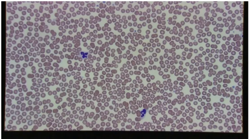
An example of this in our dataset is the voc-18-bl-1 video as shown in Figure 2.3. The high density in the number of blood cells results in a lot of occlusion and truth count challenges. It is because of such videos that we created the human-computer hybrid ground truth extraction process; a person identifies and marks the objects and the computer counts the marks.

(49)

Figure 2.3: The high object density challenge fromvoc-18-bl-1 video.

2.1.3

Scale

The problem of scale results when some of the objects of interest are close to the video recording equipment while others are further away. While the objects are the same, their size and amount of features available differs. The objects closer to the camera appear bigger while the ones further away appear smaller. As such, the success of object counting algorithms in detecting this relies on the features used to identify the objects.

The challenge in creating truth count comes from not knowing how small the objects should be before they are ignored. Figure2.4shows the scale problem invoc-18-bd-14

video where some of the birds are flying and some of them are sitting down on the water further from the camera. This video actually presents a very extreme case of this problem as some of the birds are so small that they show no discernible features. In this thesis, the ground truth for this video was created by only tagged the birds which were flying as their features were clearly visible. But even some of the flying birds had to be ignored as they were too far from the camera.

2.1.4

Vanishing Point

Situations where the camera is tilted forward as it moves across the objects of interest does not only create a scale problem, it also creates a vanishing point problem.

(50)

CHAPTER 2. DEVELOPMENT OF A VIDEO OBJECT COUNTING DATASET

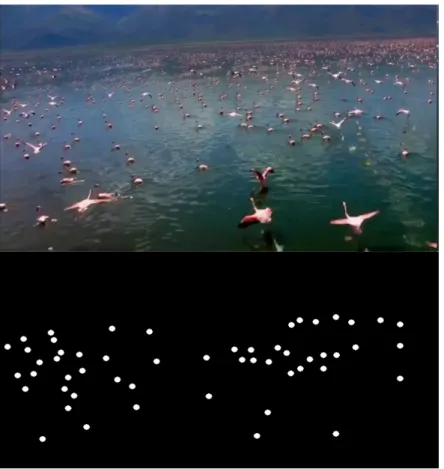
Figure 2.4: The scale challenge as seen in voc-18-bd-14 video with the binary image representation of the ground truth.

Depending on the number of objects, the inter-object occlusion and partial visibility occurs. This challenge can be seen in Figure 2.5 where the video has so many birds that the vanishing point problem merges the birds into a mass of pink. This results in a problem for both ground truth and counting algorithms. It is impossible to estimate the number of birds in the pink mass. For this video, the ground truth was created by using a similar approach to the occlusion problem discussed above. We tagged the birds as long as they can be visually separated from the pink mass.

2.1.5

Complex Background

In this thesis, we refer to complex backgrounds as backgrounds that have a wide range of characteristics such as colours, texture and other objects. This complexity

(51)

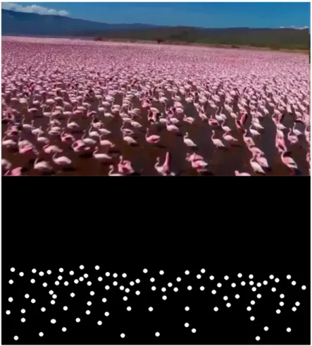
Figure 2.5: The vanishing point challenge in voc-18-bd-18 video with the binary image representation of the ground truth.

becomes a problem when the features in the background are similar to some of the features in the objects of interest. An example of such situation can be seen in Figure

2.6. In Figure 2.6a, there is a lot of a black and white colours in the background which are also present on the ducks. This is also the case in Figure2.6bwhich has the centre of the blood cell being very similar to the background. This problem does not affect the creation of the ground truth, the object counting algorithms would have to handle such problems and be able to separate the background from the foreground.

(52)

CHAPTER 2. DEVELOPMENT OF A VIDEO OBJECT COUNTING DATASET

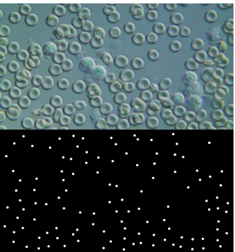
(a) The complex background from clutter in voc-18-bd-6 video.

(b) Complex foreground invoc-18-bl-3 video when the object colours are similar to the background.

Figure 2.6: Examples of complex background challenges in our dataset.

2.1.6

Complex Foreground

A complex foreground problem commonly appears when dealing with animate and deformable objects. In our dataset, flying birds offer this challenge and a lot of the videos have flying birds. The challenge is that since objects are deformable, they

(53)

can have different appearances in the frames. Also since they are animate, they can rotate and change shape providing different features. As such, depending on how flexible the features used by object counting algorithms are, some of the objects can be missed.

This problem does not necessarily provide a challenge for ground truth extraction as humans are very good at identifying objects even poorly defined ones. In addition to showing scale challenges, Figure 2.4 also presents a good example of of complex foreground. While the birds sitting in the water are a good example of this problem, the flying birds also present the challenge depending on the position of their wings in the frame.

2.2

Ground Truth Benchmark

Extracting the ground truth from the video frames requires human interaction. While the option to use people to count the objects was available, it would suffer from the usual human related problems such as fatigue, mistakes and slowness, especially when counting objects in high object density videos such as in Figure2.3. These problems were circumvented by using a hybrid human-computer process to extract the ground truth. This process relies on the ability of humans to identify accurately objects in a wide variety of situations including inter-object occlusions while computer algorithms can quickly and accurately count well defined objects. The task of getting well defined and accurately identified objects was done by a person. While a person has to actually identify the objects, they do not have to actually count them. Identifying the objects is considerably easier for humans than actually counting them.

In creating the ground truth, we first extract he frames from the video using Listing

A.5. Each frame needs to be processed independently using an image editing software to tag each object with a white dot. The tagged image is then thresholded to remove all the other colours save for the white dots. The final product of this process is a binary image that can be processed by a computer to count the number of white dots on a black background (Figure 2.7).

(54)

Figure