Separating Selection From Spillover Effects: Using the Mode to Estimate the Return to City Size
Hugo Jales
Department of Economics and Center for Policy Research Syracuse University Syracuse, New York, 13244-1020
Phone: (315) 412-8764 [email protected]
Boqian Jiang Amazon Inc., Seattle
[email protected] Stuart S. Rosenthal
Maxwell Advisory Board Professor of Economics Department of Economics and Center for Policy Research
Syracuse University Syracuse, New York, 13244-1020 Phone: (315) 443-3809
[email protected] December 29, 2020
Helpful comments are gratefully acknowledged from seminar participants at Camp Econometrics, the Urban Economic Association conference in Vancouver, the Institute for Economics at Barcelona,
AREUEA International conference at Jinan University, the NBER urban workshop, the Cleveland Federal Reserve Bank, and the University of Colorado. We also thank Nate Baum-Snow, Pierre Philippe Combes, Laurent Gobillon, David Green, Tom Holmes, Carlos Martins-Filho, Daniel McMillen and Ronni Pavan for helpful comments. All errors are our own.
Abstract
We estimate the return to city size using a new approach to test for selection. For single-peaked factor return distributions, dropping out low-performing agents causes the CDF at the mode to shrink but the mode does not shift. If instead selection extends beyond the mode, elasticity conditions govern the extent of modal shift. Estimates for U.S. MSAs confirm that for skilled workers, selection on unobserved factors contributes to higher productivity in larger cities. Among men with high school education or less,
however, selection is absent, and doubling MSA size increases mean and modal wage by 3.5%.
JEL Codes: R00, J30, C24
1. Introduction
Despite broad consensus that cities are centers of productivity and growth (see Rosenthal and Strange (2004) and Combes and Gobillon (2015) for reviews), the degree to which this arises because talented workers and companies select into large city markets remains uncertain. On the one hand, it is easily documented that cities tend to be skilled places based on observed levels of education (e.g. Bacolod et al (2009), Glaeser and Mare (2001)). More challenging is to confirm whether workers and firms sort into larger cities on the basis of unobserved skill. This uncertainty complicates efforts to estimate the productivity effects of urbanization and obscures answers to fundamental questions. Do cities cause companies to be more productive? Should urbanization be encouraged?
In this context, several recent studies have begun to offer evidence that in some settings sorting based on unobserved skill may not be very substantial, if even present. Combes et al (2012), Baum-Snow and Pavan (2012), Eeckhout, Pinheiro and Schmidheiny (2014), de la Roca and Puga (2017), and de la Roca et al (2020) all contribute to this view. Nevertheless, for a given sample of workers and firms, the potential for selection based on unobserved talent to contribute to urban productivity remains compelling. As with selection based on observables, unusually talented workers may be drawn to large cities by the intensity of urban life (e.g. Glaeser and Mare (2001), Rosenthal and Strange (2008), Combes et al. (2008), de La Roca (2017), de la Roca and Puga (2017)). Cities are also expensive places in which to live and conduct business, conditions that may cause unusually low performing workers and companies to drop out of urban markets (e.g. Rosenthal and Strange (2012), Combes et al. (2012), Black et al (2014)).1
Motivated by recent studies that draw on the shape of factor return distributions for identification (e.g. Saez (2010), Combes et al (2012), Kleven (2016), Jales and Yu (2017) and Jales (2018)), this paper develops a new approach to test for whether selection based on unobserved factors contributes to urban productivity. Our model applies to settings in which the latent return distribution is single peaked with a
1 Common approaches to dealing with the endogenous selection of workers and companies into different sized cities include the use of pseudo-random experiments (e.g. Ahlfeldt et al (2015), Greenstone et al (2010)), instrumental variables (e.g. Rosenthal and Strange (2008)), and structural methods (e.g. Baum-Snow and Pavan (2012)). Different from such strategies, Combes et al (2012) draw on the shape of the factor return distribution.
2 well-defined interior mode, characteristics that are typical of log wage and earnings patterns (e.g.
Chotikapanich et al (1997), Clementi and Gallegati (2005), Lopez et al (2006), and Sala-i-Martin and Pinkovsky (2009)). In such instances, if selection causes only low performing agents to the left of the mode to drop out of large city labor markets, the CDF evaluated at the mode will shrink and modal productivity will be unaffected by selection. In more general cases where selection extends to the right of the mode, we assume a linear monotonic selection process. In this instance, under plausible assumptions (to be clarified later), evidence that the CDF evaluated at the mode declines with city size still suggests that selection disproportionately causes low performing agents to drop out of large city markets, while elasticity conditions govern the extent to which selection causes modal productivity to shift.
The ideas above point to three complementary regressions that we estimate. The first regresses the CDF of modal factor return in the city on log city size and is intended as a diagnostic tool. As noted above, evidence of a negative city size effect indicates that selection is present and occurs more to the left of the mode. The second and third regressions replace the dependent variable with the log modal factor return in the city and the log mean factor return in the city, respectively. If the CDF regression indicates that selection is absent, the second and third regressions identify parameters of the productivity spillover function. If instead the CDF regression indicates that selection is present, then both the mode and mean estimates of the return to city size are upward biased. In that instance, for a linear monotonic selection process we show later in the paper that modal bias shrinks as the mode becomes more sharply defined, and approaches zero as the underlying factor return distribution converges to a Laplace.
We use three data sets to illustrate our approach and in each case first condition out the influence of observables. For the first application, we consider law firm productivity for all law firms in the United States, drawing on establishment level data from Dun and Bradstreet. We assume that lawyers discover through experience whether the rewards from running their own firm dominate working for someone else’s firm, and also that weak performing law firms eventually close. Operating costs and the intensity of nearby competition are also assumed to increase with city size. Given these assumptions, we expect weaker companies to drop out with higher frequency in larger cities.
3 We also apply our model to individual-level wage rates for married full-time working women age 25-55 who are white, non-Hispanic and native born, drawing on data from the 5 percent file of the 2000 U.S. census (obtained from IPUMS). It is well-established that married female labor supply is elastic so the decision to work full time my be sensitive to threshold effects (e.g. Heim (2007); Blau and Kahn (2007)).2 Consistent with this view, Black et al. (2014) argue that higher commuting costs in large cities discourage married women from working. Married female labor supply decisions may also affect choice of metropolitan area as in Costa and Kahn (2000). For both reasons, the observed relationship between city size and married female wages seems likely to be sensitive to selection.
Our third application focuses on male full-time workers age 25-55 who are white, non-Hispanic and native born, also drawing on the 2000, 5 percent U.S. census. Previous literature suggests that for this sample, the decision to work is highly inelastic (e.g. Heim (2007); Blau and Kahn (2007)) but selection effects could still arise because of migration and location decisions.
For each of the samples described above, factor return distributions after having conditioned out effects from observables are strongly single peaked with an interior mode. We argue that under plausible assumptions about the shape of the unobserved selection function, this assures that the underlying latent return distributions are similarly strongly single peaked. Given this argument, evidence indicates that for several of our sample populations, the CDF regressions yield compelling evidence that selection
contributes to higher productivity in larger cities. This includes older law firms and both male and female college educated workers. Evidence of selection is less compelling for women with limited education. In contrast, for men with a high school degree or less, there is convincing evidence that selection is absent.
Related estimates of the return to MSA size are also revealing. For older law firms that have survived the initial weeding out effects, the modal estimated return from doubling city size is
approximately 1.16% compared to 1.63% at the mean. For the wage models, among women and men with
2 Based on 1999-2001 CPS data, Blau and Kahn (2007) find that the elasticity of annual working hours with respect to own log wage is 0.357 for the married women and 0.046 for the married men. Moreover, the elasticity of annual working hours with respect to spouse’s log wage is -0.192 for the married women and -0.006 for the married men.
4 a college degree, the estimated modal return to MSA size is roughly 2.4% and 2.1%, respectively, versus 4.3% and 4.5% at the mean. In principle, these spreads between mode and mean effects could arise from two sources. One is dilation (e.g. Combes et al, 2012) if high performing individuals derive greater productivity boosts from operating in larger MSAs, causing the mean productivity gain from city size to increase relative to the mode. We do not rule out this possibility. The other is selection, which our CDF regressions confirm is present, causing low performing individuals to disproportionately drop out of large city labor markets. Given evidence in our data of strongly single-peaked distributions, the mode will tend to be less sensitive to selection than the mean (a point we address later in the paper), which will also cause the mean to increase relative to the mode.
A different pattern is present for male workers with a high school degree or less. For this sample, the CDF regression suggests that selection is absent, and the estimated return to MSA size is roughly 3.5% at both the mode and mean. We argue later in the paper that this combination of estimates indicates that dilation is not present and that doubling city size causes wage to increase by 3.5%.3
We should emphasize that the mode provides especially robust evidence of whether selection is present and can be used as a diagnostic tool. Modal shift, however, can still affect estimates of the return to city size, but to a degree governed by well-defined elasticity conditions. In drawing on the mode in this fashion, our paper is related to work by Jales (2018), Jales and Yu (2017), Saez (2010), Kleven (2016) and others that use the shape of a density function to help identify underlying causal relationships.4 It is also related to Combes et al (2012) which is the only other paper we are aware of that uses distribution methods to evaluate the returns to city size.5 Combes et al. (2012) specify a selection process in which
3 For the female high school or less wage sample, mode and mean estimates of the return to city size are 3.3% and 3.9%, respectively, close to that for low-skill men. In this instance, evidence of selection is present.
4 Our focus on the mode has relatively few precedents. Lee (1989) showed that the mode from a truncated distribution can be a consistent estimate of the conditional mean from the non-truncated distribution. Our work is also related to a limited modal regression literature in statistics and econometrics (Huang et al. 2013; Yao and Li, 2014; Chen et al., 2016, Honore, 1989). Cardoso and Portugal (2005) show that modal wage is a better measure of the central tendency of a wage distribution when there is collective bargaining. Bound and Krueger (1991) and Hu and Schennach (2008) discuss how to use mode to account for certain forms of reporting errors.
5 The vast literature on agglomeration economies has instead focused almost exclusively on mean returns. See Rosenthal and Strange (2004) and Combes and Gobillon (2015) for reviews.
5 companies drop out when factor productivity is below a common threshold. Using TFP data on French manufacturing plants, establishments are grouped into two categories based on large versus small city location, and model parameters are recovered by minimizing the mean squared deviations between TFP quantiles for the two groups.6 Relative to our approach, the quintile approach used by Combes et al (2012) has the appeal of not imposing any restriction on the shape of the underlying factor return
distribution. However, it is more computationally demanding to implement and imposes a threshold form of selection. In contrast, our approach provides a simple test for selection and, if priors suggest that selection is primarily left of the mode, our approach yields estimates of the modal return to city size without needing to impose any structure on the selection process.7
We proceed as follows. The next section develops our model. Section 3 describes the data and summary statistics. Section 4 discusses how to measure the mode. Section 5 presents the results and Section 6 concludes.
2. Model
This section presents our modeling framework. Notation used throughout the section includes the following. A worker’s skill endowment is given by Y which differs across workers and is set equal to 1 for the least skilled individual in the population. City population is given by S, where S is also set equal to 1 for the smallest city in the system of cities. In logs, these measures are expressed as y and s. The terms f0(y) and fs(y) are then used to refer to the distributions of log productivity among individuals in the
smallest city and a city of size s. Except where noted, f0(y) and fs(y) are assumed to be continuous and
differentiable.
6 As noted earlier, Combes et al. (2012) do not find evidence of selection and conclude that higher manufacturing productivity in larger French cities arises primarily from spillover effects. This is similar to our estimates for low-skilled men but different from the other populations that we analyze.
7 Combes et al (2012) also draw on the entire productivity distribution whereas we focus only on the mode. This makes our estimates less precise.
6 2.1 Productivity spillovers from city size
Suppose that the only force that causes f0(y) to differ from fs(y) are productivity spillovers arising
from city size. Both here and in the empirical work to follow, spillover effects in a city of size s are measured relative to spillovers in the smallest city in the system. To simplify notation, for a given skill endowment, productivity in the smallest city (s = 0) is given by y while productivty in a city of size s > 0 is given by 𝑦 .
Large city agglomeration economies are assumed to take a linear form that preserves an individual’s productivity rank within a given city, similar to the approach in Combes et al (2012) and Firpo (2007).8 For a given skill endowment y, productivity in a city of log size s is given by,
𝑦 𝛽 𝑠 1 𝛽 𝑠)𝑦 , (2.1)
where the spillover function is assumed to be common across all workers. In the absence of spillovers, 𝛽 = 𝛽 = 0 and 𝑦 = y, in which case an individual’s productivity is the same in all cities. If instead doubling city size increases productivity by a common percentage for all workers, 𝛽 0, 𝛽 = 0, and fs(y) shifts to
the right relative to f0(y). For this case, it is helpful to note that relative productivity for low and high
skilled individuals, represented here by Yhigh/Ylow, is unaffected by city size. Nevertheless, a “linear
dilation” effect is still present because the difference in the level of productivity between high and low skill workers (Yhigh – Ylow) increases with city size at rate 𝑆 since 𝑌 𝑆 𝑌. If in addition 𝛽 > 0, a
“relative dilation” effect will also be present because the ratio Yhigh/Ylow will increase with city size
causing fs(y) to become right skewed with an elongated right tail. In the discussion to follow, we will
periodically refer to linear and relative dilation as defined here.
For the spillover function specified above, the cumulative distribution function (CDF) for
productivity up to a given skill endowment, 𝑦, is the same in each city, denoted as F0 for the smallest city
and Fs for a city of log size s,
8 The rank preservation assumption is standard in the literature of quantile treatment effects. See Firpo (2007) and the references therein for discussion.
7
𝐹 𝑦 𝑦 𝐹 𝑦 (2.2)
Substituting for ys from expression (2.1) and taking derivatives with respect to y, the relationship between
large and small city productivity densities is given by,
𝑓 𝑦 𝑓 (2.3)
Our most important modeling assumption in the empirical work to follow, referred to as Assumption 1, is given by:
Assumption 1: f0(y) is single peaked with a well defined mode at an interior location.
In conjunction with spillover effects as modeled in (2.3), this assumption has important implications for the shape of productivity density functions in large versus small cities. To illustrate, we took 10,000 random draws of y from a normal distribution, mirroring assumptions in the labor and agglomeration literatures that typically treat wage and earnings distributions as log-normal. We set the standard deviation of the distribution to 0.4, a value small enough to conveniently plot the distribution. We also set β0 = 0.5 and β1 = 0.3, implying that doubling city size boosts productivity by 50 percent regardless of
skill and an additional 30 percent with a doubling of worker ability. These values are purely for
illustrative purposes and make plotting of the distributions to follow convenient while also allowing us to higlight key principles.
Figure 1 traces out the simulated productivity density functions for two city sizes, large (the dashed red line) and small (the solid black line) based on the parameters above and setting s = 1 for the large city case. Notice that for large cities, the density function is right shifted with an elongated right tail (right skewed) relative to the density function for small cities. The large city density is also flatter, with a lower density for any given level of productivity, and a right shifted mode. A positive value for β0 shifts the large city log productivity distribution along the x-axis by β0 units while preserving its shape. This is apparent from (2.1) and (2.3). In (2.1), the derivative of ys with respect to β0 is s, while from (2.3) the large city density with β1 = 0 is f0(y - β0s). Observe, however, that even though β0 is just 0.5, the mode in
8 Figure 1 shifts by a larger amount, from 0.85 in small cities to 1.55 in large cities. The additional
rightward shift in the mode is because β1 > 0 draws the mode further to the right, although not
immediately apparent from a casual viewing of (2.3). As is evident in the figure, the mode in the large city density is also not as pronounced relative to a smaller city. This is also a consequence of β1 > 0, which flattens the density function by shifting mass from the center of the distribution into the elongated right tail, and bearing in mind that the density function must always integrate to 1.
2.2 Selection effects
This subsection considers the influence of selection effects that govern participation in a given city labor market. Suppose that small city residents participate in the labor market with probability 1 regardless of skill, or π0(y) = 1, where π0(y) is the probability of participating. If in large cities πs(y) is also
constant with πs(y) = p < 1, then participation in the large city labor market is independent of skill
endowment and in that sense is random. More relevant to our context is the possibility that participation in larger city labor markets increases with skill, which we assume to occur in a linear fashion:
Assumption 2: The probability of selecting into and participating in a size-s city labor market is approximated by a linear specification,
𝜋 𝑦
𝑎 𝑏𝑦, for y 𝑦
𝑝 1 , for y 𝑦 (2.4)
with 0 𝜋 𝑦 1, b > 0.
In (2.4), the term 𝜋 𝑦 is indexed by s to indicate that the selection probability for a given y differs with city size. Implicitly, a, b, p, and 𝑦 are also indexed by s but the subscript on these terms is suppressed to simplify notation. Assumption 2 also makes explicit that πs(y) reaches an asymptote at 𝑦 with p ≤ 1 since
πs(y) can never exceed 1.
Assumption 2 captures the sense that operating costs are higher in larger cities and/or the environment more competitive. This discourages weaker workers and companies from participating in larger city markets (e.g. Combes et al (2012)).
9 Allowing for selection effects as above, and also the possibility of productivity spillovers,
expression (2.3) becomes,
𝑓 𝑦 𝑓 (2.5)
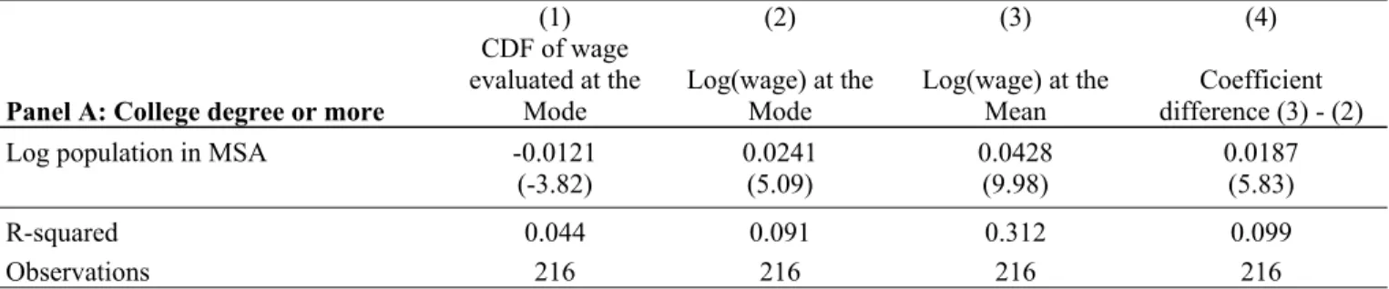
where 𝑐 𝜋 𝑢 𝑓 𝑢 𝑑𝑢 ensures that the conditional density in the large city integrates to 1.9 We illustrate the qualitative effects of selection in Figures 2a and 2b using the same simulated data as for Figure 1, first without and then with spillovers. As before, we assume only two cities, small and large. In Figure 2a, we set β0 = β1 = 0, consistent with the absence of agglomeration economies. The
πs(y) function is specified so that it increases up to a value of 1 at the mode of the latent distribution (at y
= 0.85).10 Imposing these features, ten percent of the simulated work force is selected out of the large city labor market, all of whom have skill levels to the left of the mode. The important point to recognize in Figure 2a is that even though all selection occurs to the left of the mode, selection steepens the slope of the large city density function on both sides of the mode while also increasing the height of the mode. Together, these effects cause the mode in the productivity density function to become more pronounced.
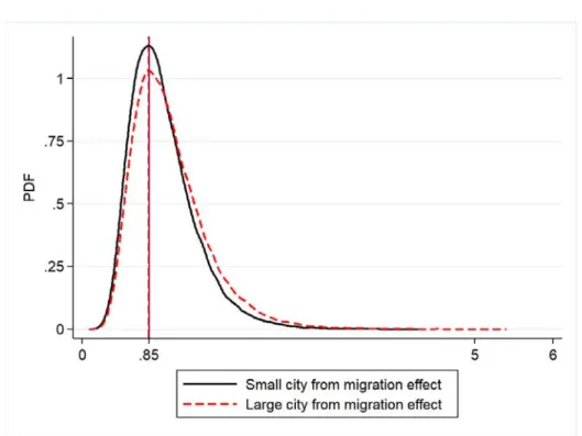
Figure 2b illustrates the combined influence of threshold and spillover effects, with density plots for small and large cities in the upper portion of the figure and corresponding CDF plots in the lower portion. In this instance we set β0 and β1 to the values used in Figure 1 and specify πs(y) as in Figure 2a.
Notice that the influence of threshold effects on the density functions for small and large cities is difficult to discern relative to the pattern in Figure 2a. That is because β1 > 0 flattens and right-skews the
distribution causing the mode to become less pronounced. This offsets the tendency for threshold effects to accenuate the mode. On the other hand, because all selection out of the large city distribution is to the left of the large city latent density mode, the CDF evaluated at the large city mode must shrink relative to
9 Notice that for the special case when selection is independent of y, πs(y) = 𝑐 = p, and in the absence of spillover effects (𝛽 = 𝛽 = 0), expression (2.4) simplifies to fs(y) = f0(y).
10 More precisely, we set π(y) = - 0.27 + 1.5y for y ≤ 0.85 and π(y) = 1 for y ≥ 0.85. Specified in this manner, πs(y) = 0 for the lowest level of y in the simulated sample and approaches 1 asymptotically from below at y = 0.85.
10 the CDF at the mode in the small city distribution. This is confirmed in the lower portion of the figure where the CDFs evaluated at the small and large city modes are, respectively, 0.34 and 0.27.
2.3 By how much does the mode shift in response to selection?
This section establishes conditions that govern the extent to which selection will cause the mode to shift. This will help to further clarify conditions under which the CDF evaluated at the mode is an effective device to detect selection. Awareness of the potential for modal shift is also important when using the mode to control for selection effects.
2.4.1 Elasticity condition
Suppose that selection effects are present but agglomeration economies are not. Then β0 = β1 = 0, and the conditional density in (2.4) becomes,
𝑓 𝑦 𝑓 𝑦 . (2.6)
The question we seek to answer is by how much selection may shift the mode of the conditional density fs(y) relative to the unconditional density f0(y). Since f0(y) is assumed to be differentiable and single peaked, its slope at the mode is zero. Differentiating (2.6) with respect to y and setting the derivative to zero, the modal value for y (denoted by ym) in the conditional density, fs(y), is assumed to be unique and
must satisfy,
𝜓 , 𝜓 , (2.7)
where 𝜓 , ≡ ′ and 𝜓 , ≡ are the semi-elasticities of the selection and latent density
functions, respectively. Note that these expessions vary with city size but the s subscripts are supressed to simplify notation.
11 Expression (2.7) indicates that at the mode of the conditional distribution, a small change in y yields equal magnitude but opposite signed percentage changes in the selection probability and the density of y. Multiplying both sides of (2.7) by y (for y ≠ 0) this can also be expressed as an elasticity condition,
𝜉 , 𝜉 , (2.8)
with 𝜉 , %∆
%∆ and 𝜉 , %∆
%∆ , where the s subscripts are supressed once again.
11 In some parts of the discussion to follow it is helpful to characterize modal shift using the semi-elasticity condition while in other instances the elasticity condition is more informative.
2.4.2 Magnitude of mode shift
Below are four propositions that govern the amount by which the mode may shift in a city of size s in response to selection effects relative to the latent density. The first case is relevant to when all selection occurs on just one side of the mode. In this instance, it is not necessary to specify any structure for the selection function.
Proposition 1: Given Assumption 1, if selection only removes mass from one side of the latent density mode ym then ...
(i) The mode of the conditional density function does not shift.
(ii) The CDF evaluated at the mode will decline if selection occurs to the left of the mode and will increase if selection occurs to the right of the mode.
Proof: By definition, the mode of a single-peaked density function has the highest density. Removing mass only from one side of the mode scales up the density elsewhere in the distribution – including at the original mode – by a common factor so that the conditional density integrates to one. This ensures that the mode does not shift.
The second case includes situations in which, over a relevant range of y, the selection probability πs(y) is a constant less than 1, indicating that selection is random. In this instance, the selection function
will be flat and 𝜉 , 0.
11 The elasticities above express the percent change along the vertical axis in response to a percent change along the horizontal axis. This is the inverse of familiar demand and supply elasticities. The elasticities in (2.8) are specified as above because y is the exogenous determinant of f and π.
12 Proposition 2: Given Assumptions 1 and 2, if the selection probability is constant for y > yp
where yp is to the left of ym, then the mode will not shift and Proposition 1 will hold even when
mass is withdrawn from the mode.
Proof: If πs(y) = p < 1 from a point yp to the left of the mode and beyond, then selection is random for all y
> yp. Thus, the rank order of the density at the mode will be preserved and the mode will not shift
regardless of the shape of the selection function.
Consider now a third and more general case in which the selection function increases with y and reaches an asymptote p to the right of the mode at yp > ym. In this instance, additional structure must be
imposed on both the density and selection functions in order to characterize the degree to which the mode will shift in response to selection. For the density function we replace Assumption 1 with a generalized error distribution (GED) and consider two cases based on the shape parameter, κ, as defined below.
Assumption 3: f0(y) belongs to the family of symmetric, generalized error distributions (GED):
𝑓 𝑦 𝑒 (2.9)
where 𝜇 is the center of the distribution (equal to the mode, median and mean, and ym above). The
scale parameter σ governs the degree of dispersion in the distribution, κ is a shape parameter that affects the degree to which the mode is sharply defined, with range from 0 to ∞, and 𝛤 denotes the gamma function.
For this density function, κ = 1/2 corresponds to the normal distribution. For κ = 1, the resulting
distribution is a double exponential or Laplace distribution which has a sharply defined mode, and for κ < 1/2 the distribution has a flatter mode than the normal. In the limit, as 𝜅 → 0, f0(y) converges to a uniform U(μ - σ, μ + σ) and at the other extreme, as 𝜅 → ∞ , f0(y) becomes degenerate with all mass concentrated at a single value for y.
In the discussion to follow we consider two cases based on whether κ is strictly less than 1 or κ ≥ 1. For the former, elasticity conditions govern modal shift. However, when κ ≥ 1, the GED has a non-differentiable point at the mode and the mode is as least as sharply defined as for the Laplace. For this case, we show in Appendix C that the mode does not shift for any continuous and differentiable selection process like the one described in equation (2.4).
13 Recall that equation (2.4) makes explicit that πs(y) reaches an asymptote p ≤ 1 at 𝑦 . If 𝑦 is to
the right of the latent density mode ym, the semi-elasticity and elasticity for the selection function are
given, respectively, by:
𝜓 , , for 𝑦 𝑦 0, for 𝑦 𝑦 . (2.10a) 𝜉 , 𝑦 , for 𝑦 𝑦 0, for 𝑦 𝑦 . (2.10b)
In the discussion to follow, it will become apparent that if 𝜓 , and 𝜉 , are in the inelastic range between 0 and 1, the degree to which the mode shifts in response to selection is reduced, and in that sense the mode is more robust. For 𝜉 , , a value in the inelastic range is always assured given the selection and
density functions specified in (2.4) and (2.9). For 𝜓 , , an inelastic value is not assured as a general principle but is very likely to hold for plausible specifications of the selection function. We elaborate on these points before proceeding.
Recall that πs(y) is a probability with range between 0 and 1. Also, skill level (Y) is non-negative
and is defined (without loss of generality) as having a minimum value of 1 with y having a corresponding minimum of 0. From (2.10), this implies that πs(y) = a, with 0 ≤ 𝑎 1. For b > 0 (nonrandom selection),
from (2.10b) the elasticity 𝜉 , has a maximum of 1 when a equals zero and shrinks towards zero at a rate
–by(a + by)-2 as a increases towards 1. This confirms that 0 ≤ 𝜉
, 1.
The semi-elasticity 𝜓 , is in the inelastic range as long as 𝜋 𝑦 > 𝜋 ′ 𝑦 = b. For plausible selection functions this condition is likely hold since 𝜋 𝑦 equals the integral of 𝜋 ′ 𝑦 from 0 to y. Moreover, 0 ≤ 𝜓 , 1 is assured for y > 1 and also if a > b in instances when 0 ≤ y < 1.12 Although a > b need not hold as a general property, it is likely to hold for a selection function governing participation in
12 From (2.10a), note that 𝜓
14 large city labor markets. New York city, for example, accounts for a large share of U.S. national
employment, implying “large” a. A wide range of skill in the workforce is also present in cities of all sizes in the United States, implying “small” b. For all of these reasons, the semi-elasticity above is likely in the inelastic range.
Bearing these points in mind, the extent to which the mode shifts in response to selection is governed by the parameters a, b, σ and κ, subject to the conditions in (2.7) and (2.8). These and related principles are formalized in Proposition 3.
Proposition 3: If assumptions 2 and 3 hold, the selection function reaches an asymptote p at 𝑦 > 𝑦 , and k < 1, then …
(i) Expressions (2.6) and (2.7) are satisfied at a value for y that is characterized by:
𝑦 𝑦 𝜎 𝜓 , (2.11a)
where 𝜓 , = , .
(ii) The mode of the conditional density in city s, denoted by 𝑦 , , is characterized by:
𝑦 , 𝑚𝑖𝑛 𝑦 , 𝑦 𝜎 𝜓 , (2.11b)
(iii) For normalized data with 𝜎 = 1, this simplifies to:
𝑦 , 𝑚𝑖𝑛 𝑦 , 𝑦 𝜓 , (2.11c)
Proof: See appendix A.
Proposition 3 has several subtle features. If the selection function hits an asymptote before the elasticity conditions in (2.7) and (2.8) are satisfied, then the mode changes by 𝑦 - ym . In this instance, if
𝑦 is close to ym then selection will have little effect on the mode. If instead 𝑦 is sufficiently large so that
the elasticity condition determines the conditional mode, then the mode shifts to the right by an amount governed by 𝜎 𝜓 , , where 𝜎 and k determine the degree to which the mode is sharply defined.
15 Suppose now that selection is random, as with the case associated with Proposition 2. Then 𝜓 , = 0 and (2.11) confirms that the mode does not shift. If instead, 𝜓 , 0, then for a given shape
parameter k, as the scale parameter 𝜎 of the latent density increases, the distribution of y becomes more spread out and (2.11b) indicates that modal shift increases.
Recall now that for plausible linear selection functions that govern participation in large city labor markets, 𝜓 , is likely less than 1. Consider also what happens as k approaches 1 from below so that the GED converges to a Laplace distribution. From (2.11b), provided 𝜎 < 1, modal shift goes to zero including for normalized data for which 𝜎 = 1 as in expression (2.11c). If instead 𝜎 > 1, the pattern is more complicated. In this instance, as k approaches 1 from below, modal shift is approximately given by
𝜎𝜓 , . This goes to zero if the product σ𝜓 , < 1, but becomes large if σ𝜓 , > 1. This last example illustrates that both 𝜎 and k govern how well defined the mode is when considering the influence of selection on modal shift.13
For the normal distribution, k = ½. In this instance, (2.11b) indicates that the change in the mode will be characterized by 𝜎 𝜓 , . Given how often normal distributions are relevant to economic data, this case is of particular interest.
The special case of the uniform distribution is also instructive. In the limit as k goes to 0, the GED converges to a uniform distribution, U( 𝑦 - σ, 𝑦 + σ). In this extreme case 𝑓 𝑦 becomes a constant equal to q for the relevant range of y. From (2.5) it follows that 𝑓 𝑦 𝜋 𝑦 . The
conditional density function therefore takes on the shape of the selection function scaled by q/c. With b > 0, the mode of fs(y) must shift all the way to the right edge of the distribution. This is also confirmed by
(2.11b), where the shift in the mode is given by σ when k = 0.
13 Substituting for 𝜓
, with , above, it is also clear that σ𝜓 , is more likely to be less 1 as the mode of the latent density function takes on a larger value.
16 It is also worth emphasizing that when 𝑦 is not binding, (2.11) will only have a closed form solution for 𝑦 , in select cases. This includes k = 0 as just discussed. A closed form solution is also
obtained if the selection process is exponential, with 𝜋 𝑦 𝑒 . In this instance the mode will shift by 𝜎𝜉 , , where the selection elasticity simplifies to 𝜉 , = b.
Consider now the shift in the mode relative to the shift in the mean.Under our modeling assumptions, the change in the mean arising from selection effects is approximately given by , where 𝜇 is the unconditional mean of y and the other terms are as defined in (2.10) (see Appendix B for a derivation). This approximation is exact if the selection function does not hit an asymptote within the domain of the latent productivity distribution.14 If 𝑦 is far to the right of 𝑦 , the shift in the mean
compared to the mode depends on the size of relative to 𝜎 𝜓 , . Both of these expressions collapse to zero when selection is random (b = 0). It is also worth noting that the shape parameter κ does not affect the shift in mean but does affect modal shift by governing the degree to which the mode is well defined. For distributions with sufficiently small 𝜎 and large κ the mode will shift by less for reasons described above. As the density function becomes flatter, however (with small κ), or more spread out (with large 𝜎), the mode becomes less well defined, and selection will eventually cause the mode to shift further to the right than the mean.15 These examples reinforce a central point emphasized at the start of the paper: the mode is an effective way to detect and control for selection when the density function has a well defined interior mode. This requires distributions that are not too flat or too spread out.
Two final comments remain when considering the viability of using the mode to detect and control for selection effects. First, sample size must be large enough to yield sufficiently reliable
14 If instead the selection process can be modeled as a Tobit, as an example, the conditional mean shifts by an amount given by the familiar inverse mills ratio scaled by σ, or σ𝐸 𝑦|𝑦 0 𝜎 // , where f and F are the density and CDF of the outcome distribution and μ is the mean of y in the absence of selection.
15 Recall also that the mode also shifts far to the right when 𝜎 is large even if κ is also large, as with a Laplace distribution (for which κ = 1). In that sense, the need for a “well-defined” mode precludes distributions that are too flat as well as distributions for which too little mass is concentrated close to the mode because of large 𝜎.
17 estimates of the mode. Second, the mode needs to be of intrinsic interest in the context being considered. It captures a different part of the distribution than the mean or median, for example.
2.4.3 Identifying whether selection is present and the underlying parameters
This section highlights conditions under which estimates from our regressions to follow can be used to identify whether selection is present and also the magnitude and/or sign of the underlying
parameters of the selection and productivity spillover functions, a, b, and p in (2.9) and β0 and β1 in (2.1), respectively.
As described in the Introduction, we estimate three regressions in the sections to follow:
𝐶𝐷𝐹 𝑦 , 𝑐 , 𝑐 , 𝑠 𝑒 (2.12a)
𝑦 , 𝑐 , 𝑐 , 𝑠 𝑒 (2.12b)
𝑦 𝑐 , 𝑐 , 𝑠 𝑒 (2.12c)
where, as before, 𝑦 , is the modal log wage in MSA i, 𝑦i is the average log wage in MSA i, and si is
MSA i’s log population. The constants in these regressions capture features that are not associated with MSA size and are not of interest for that reason. Instead, it is the three slope coefficients in (2.12a-c) that are the primary focus. Conditions under which these parameters help to identify the presence of selection and the underlying selection and spillover functions are summarized below. We focus only on cases for which b ≥ 0 given priors that if selection is present unusually skilled agents will select into larger city labor markets.
Proposition 4: For the spillover and selection functions assumed in (2.1) and (2.4), estimates of (2.12a-2.12c) imply that on average across cities in the sample …
(i) If b = 0, selection removes equal mass from the left and right of the mode, and c1,1 = 0.
(ii) If c1,1 < 0, it follows that b > 0 and selection removes more mass to the left of the mode.16
16 It is worth emphasizing that c
1,1 < 0 understates evidence that selection is present. This is because although b > 0 implies that selection removes more mass left of the mode, b > 0 also pushes the mode to the right. Because the latter increases the CDF evaluated at the mode, c1,1 < 0 understates evidence of selection.
18 (iii) If 0 ≤ 𝑦 𝑦 , all systematic selection is left of the mode and the mode does not shift in
response to selection. In this instance, c1,1 approximates the loss of mass to the left of 𝑦
in response to an increase in MSA size, and c1,2 measures the causal effect of MSA size
on factor returns at the mode.
(iv) If c1,1 = 0, then selection is absent in the sense defined in (i), and c1,2 and c1,3 measure the
causal effect of MSA size on factor returns at the mode and mean, respectively. In addition, β0 and β1 are identified as,
𝛽 𝑐 , 𝑐 , 𝑐 ,
𝑦 𝑦 𝑦
𝛽 𝑐, 𝑐 ,
𝑦 𝑦
where 𝑦 and 𝑦 are based on values for the reference city (e.g. the smallest city). (v) If c1,1 < 0 and 0 ≤ 𝑦 𝑦 , then c1,2 and c1,3 are both biased upwards by selection and
provide upper bounds on the causal effect of MSA size on productivity at the mode and mean, respectively.
In viewing the comments above, recall that because the productivity spillover function in (2.1) preserves an individual’s rank in the productivity distribution, spillover effects do not affect the CDF evaluated at 𝑦 . This leads to statements (i), (ii), and (iii).
In statement (iv) with c1,1 = 0, the regressions specified in (2.12b) and (2.12c) yield estimates of
the causal impact of MSA size on modal and mean productivity, respectively. In this instance, taking derivatives of (2.1), (2.12b) and (2.12c) with respect to s and solving yields expressions for β0 and β1.17 From those expressions, it is worth noting that if c1,2 = c1,3, then relative dilation is absent with β1 = 0 and c1,2 = c1,3 = β0.
For statement (v) with c1,1 < 0 and selection extending beyond the mode, selection causes both the
mode and the mean to shift to the right as described earlier. In this instance, c1,2 and c1,3 are both upper
bounds on the causal effect of spillover effects.
17 Taking derivatives of (2.1), (2.12b) and (2.12c) with respect to s yields, respectively, 𝛽 𝛽 𝑦, 𝑐 , , and 𝑐, . Evaluating the first of these derivatives at 𝑦 and 𝑦 yields two equations that can be solved for 𝛽 and
19 3. Data and Summary Statistics
3.1 Three datasets
Three datasets are used to estimate the returns to city size based on the model above as described in the Introduction. The first includes sale per worker at all law firms in the United States. The second sample is based on wage rates for married women who work full-time and are age 25-55, white, non-Hispanic and native born. The third sample focuses on wage rates for all men, including single and married. Each of the samples along with related summary statistics and density functions are described below. Additional details on how we measure the mode are provided in the section that follows.
For each of these samples, we first remove the influence of observables (e.g. education, age, etc. in the wage samples) so that our analysis of the presence and effect of selection is based on unobserved factors. In the discussion to follow, we show that the conditional outcome distributions for each of our samples are strongly single peaked with an interior mode, and for that reason, a good match for our modal approach.
3.2 Law firm establishment data from Dun & Bradstreet
We collected 2016 establishment-level data for all law firms in the United States (excluding Alaska and Hawaii) from the Dun & Bradstreet Million Dollar Database. The data provides information on establishment location, level of employment, sales, industry (SIC 8-digit code), year established, and other details. Compared to the Census data, an advantage of Dun & Bradstreet database is that it provides comprehensive coverage of small businesses including those with just one or two-workers.18
The data were collected in December 2016 and provide a snapshot of all law firms operating in the U.S. at that time. We use establishment-level sales per worker as a proxy for productivity, trimming
18 In our sample, there are 545,873 law establishments. Of these, 8.5% have one worker, 62.8% have two
employees, 15.0% have three workers, and 13.5% have four or more workers. In comparison, in the 2012 Economic Census, there are 186,831 law establishments in the U.S. The main reason for the difference is that Census indicates that it does not “survey very small businesses”. For details see the Census website:
20 out the top and bottom 0.1% of the data to reduce outliers.19 Certain types of law offices may be more prevalent in large cities (e.g. corporate law). Because concerns about selection stem from unobserved factors embedded in the error term, we pre-cleaned the data to difference out the average return for the primary classifications of law firms identified in the data.20 This was done by regressing individual establishment sale per worker on dummy variables for each type of 8-digit law office reported by Dun and Bradstreet. We then added back to the residual from this regression the average sale per worker for general law offices/attorneys which account for 90% of the sample. The adjusted cleaned residual has the same sample mean as in the raw data and is used as the dependent variable.
A key part of our empirical strategy is to measure the mode of the adjusted sales per worker distribution in each MSA. To ensure sufficient sample, we retain only MSAs for which all of the following conditions are satisfied: (i) more than 30 law firms age five or younger are present, (ii) more than 30 law firms over five years in age are present, and (iii) MSA total population is over 100,000. For all of the law firm models, MSA size was estimated using the 2015 American Community Survey which is approximately the same period as the 2016 law firm sample.21 Cleaning as above, we are left with 239 MSAs. The total count of law firms in the sample is 545,873 firms. Of these, 74,079 firms are young, defined as five years or less in age, and 471,794 firms are old, defined as over five years in age.22
Table 1 Panel A presents summary statistics of sales per worker for all law firms sample and also separately by age group (young and old). Based on the 25th and 75th quantiles, the majority of the sales per worker measures fall within the range of $60,000 and $85,000. Measured at the mean and different quantiles, old firms have higher sales per worker than the young firms, indicating that older law firms are more productive than younger companies.
19 Similar trimming procedure is also used in Combes et al. (2008), Combes et al. (2012) and Gaubert (forthcoming). 20 Based on SIC 8-digit codes, approximately 90% of the sample is coded as general law offices/attorneys. The remaining 10% of the sample is coded into more specialized classifications, including corporate law, family law, etc. 21 The 2013 Office of Management and Budget metropolitan area delineations are used to define MSAs.
22 Among the 545,873 establishments, age related information was missing in the D&B data for 67,358 establishments (12% of the sample). For roughly 200 of these firms, we searched the companies on the web by establishment name (which is also reported by D&B). In each instance, the establishments was over 5 years in age. For that reason, we classified all law firms in D&B with missing age information as over 5 years in age (i.e. as old establishments).
21 Figure 5 provides kernel density plots of sales per worker for the all firms sample (Panel A) as well as for the different age groups (Panels B and C for young and old, respectively). In each panel, the sales per worker distribution is strongly singled peaked (along with some secondary spikes that we return to in the following section). Panels D-F repeat these plots for law establishments in small (population < 1 million) and large (population > 2.5 million) MSAs. In each case, the large-MSA distribution of sales per worker is clearly right-shifted as compared to small MSAs.
3.3 Married white female full-time workers in the 2000 Census
The sample of female married white non-Hispanic native-born full-time workers (age 25-54) was obtained from the 2000 decennial census 5% public use micro sample (PUMS) from IPUMS.23 Full-time workers were coded as those who report working at least 35 hours per week and 40 weeks per year.24 Hourly wage was used as a proxy for productivity and was computed by dividing annual earnings by annual hours worked. As above, we trim the top and bottom 1% of the sample based on hourly wages to remove outliers.
Also analogous to above, the data were pre-cleaned to remove the influence of observables. This was done by regressing individual log wage on age fixed effects, education fixed effects, occupation fixed effects and industry fixed effects.25 We retain the wage residual from each worker and calculate the adjusted “cleaned” wage by adding back a constant that sets the mean of the adjusted wage series equal to that of the raw data sample mean. Wage data were cleaned separately for skilled (college degree or more) and low-skilled (high school degree or less) workers separately.26
23 See Steven et al., 2015 and www.ipums.org. Observations from Alaska and Hawaii were excluded.
24 We focus on full-time workers in part to reduce measurement error when calculating hourly wages which is more pronounced among part-time workers. See Baum-Snow and Neal (2009) for related discussion.
25 To be specific, there are 15 age fixed effects, 359 occupation fixed effects and 94 industry fixed effects. In the census, the most detailed version of occupation classification is at 6 digits, which is too refined for certain
occupations to have enough sample size to yield precise estimates of fixed-effects. Therefore, we choose to control for occupation fixed effects using 5-digit classification. As a robustness check, we find that controlling for
occupation fixed effects at 4-digit or 6-digit level yield similar results.
26 Using this approach, a small number of observations had negative adjusted wage. Dropping these observations did not affect our results.
22 MSA population size was estimated using the 2000 census, the same year that the wage data were drawn from.27 We retain only those MSAs for which all of the following conditions are satisfied: (i) more than 100 married female non-Hispanic white native-born workers with a college degree or more present, (ii) more than 100 married female non-Hispanic white native-born workers with a high school degree or less are present, and (iii) MSA total population is over 100,000. The data cleaning procedure leaves us a sample composed of 152,704 skilled married female workers and 153,168 low-skilled married female workers from 216 MSAs in the United States.
Table 1, Panel B provides summary statistics of adjusted hourly wage for the married female workers. Measured at the mean and each quantile, the adjusted hourly wage is higher among the skilled workers. Figure 6, Panels A and B, present kernel density plots of the adjusted hourly wage for high- and low-skilled workers. The first thing to note is that the both distributions are strongly single-peaked. The density plot for the skilled workers (Panel A) also has a longer right tail and a larger variance as
compared to the plot for low-skilled workers (Panel B). Splitting the samples into small and large MSAs, we reproduce the density plots in Panels C and D. For both groups of workers, the wage density plots for large cities is right-shifted and dilated as compared to the density plot for small cities.
3.4 Male full-time white workers in the 2000 Census
Male non-Hispanic white native-born full-time workers (age 25-54) data is also drawn from the 5% PUMS of the 2000 decennial Census. These data are cleaned in the same way as for the married female workers. This leaves us with 383,728 workers with a college degree or more and 393,598 with a high school degree or less. These workers are spread across 262 MSAs in the United States. Table 1, Panel C summarizes the adjusted hourly wage for the skilled (college degree or more) male workers and low-skilled male workers (high school degree or less).
27 The population estimate is obtained through the IPUMS website. Link: https://usa.ipums.org/usa-action/variables/MET2013#description_section
23 Not surprisingly, skilled workers have higher adjusted hourly wage than the low-skilled group, both at various quantiles and also at the mean. Figure 7, Panels A and B, display kernel density plots of the adjusted hourly wage for the two groups of male workers. In both panels, the aggregate adjusted wage distributions are again quite smooth and strongly single-peaked. Splitting the samples into small and large cities (Panels C and D, respectively), it is also evident that the wage density for large cities is right-shifted and dilated as compared to the density plot for smaller cities, similar to the patterns for the married female sample. Also similar to the female worker sample, the density plots for men in Figure 7 are quite smooth.
4. Measuring the mode 4.1 Measurement procedure
In the estimation to follow, separate modal values are first estimated for each MSA for each sample using a kernel density approach. In each instance, we use Epanechnikov for the kernel function and Silverman’s rule of thumb for selection of the optimal bandwidth.
Summary measures in Table 1 also provide some context as to reasonable bandwidths. In Panel A, notice that the inter-quartile range for the law firm sales per worker is roughly $20,000 to $25,000 for all three main samples, including all law firms, young and old. This suggests that any bandwidth larger than $10,000 would not preserve enough variation in the data to yield reliable results. In Panel B, observe that for female wages, the interquartile range of adjusted wage is $10 for the skilled married female workers and $5 for the low-skilled workers. For men the analogous measures in Panel C are $16 and $7. The range of these data suggests that a bandwidth as small as just $2 or $3 would likely be effective for the wage measures. The bandwidths selected by the smoothing algorithm are all within these ranges.28 It is also worth noting that the density plots in Figures 6 and 7 for female and male wages stratified into large and small MSAs are quite smooth. This is true both overall and in comparison to the law firm sale per worker density functions in Figure 5. To understand why, consider that each firm or individual’s skill
28 As a robustness check, we also re-ran all of the models to follow using one-half the optimal bandwidth from the kernel density routine. Results were quite close to those presented in Tables 3-5 and are not reported for that reason.
24 endowment can be expressed as the sum of a systematic component and a random component. It is
plausible to assume that the random component is drawn from a smooth single-peaked distribution. Recall also that we restrict our samples to relatively homogenous populations. We do not mix law firms with other types of establishments, for example. In the case of the wage models, we restrict the samples to white, non-Hispanic native-born full-time workers (age 25-54). As these sorts of sample restrictions become more refined, all that will remain will be random skill components.
4.2 Summary statistics for the modal values
Based on the MSA by MSA kernel density estimates, Table 2 displays summary measures for the model values of the sale per worker and wage measures for each of our samples. We emphasize that each observation in the table is a separate MSA. Observation counts differ across the samples because of the sample cleaning procedures described above.
Panel A reports values for law firm sale per worker. Regardless of age of the company, the median modal value across 239 MSAs is roughly $57,000 with a standard deviation of roughly $4,000 and range of $25,000. For female wages, the median modal wage among college educated workers is $21.30 with a standard deviation of $1.77 and a range of roughly $9. For college educated men (Panel C) wages are higher by about $5 at all points in the distribution and with a larger standard deviation of $2.1. Among workers with high school or less, differences in the distribution of modal wages for women and men are reduced and the overall distribution is shifted down. The median is close to $14 for both groups although there is more variation for men with a standard deviation of $1.5 and a range of $3.75.
5. Estimates
5.1 Young and old law firms
Table 3 presents MSA level regressions based on law firm sales per worker. Panel A reports results for the all firms sample, Panel B for young law firms (5 years or less in age), and Panel C for older firms (older than 5 years). For each panel, column (1) displays estimates from the first stage regression of
25 the CDF of sale per worker evaluated at the mode on log population of the MSA. Column (2) reports estimates from the second stage regression of log sale per worker at the mode on log population of the MSA. For comparison, Column (3) reports estimates from a regression of log sale per worker at the mean for the MSA. Column (4) reports a test of the difference between the two elasticity estimates in columns 3 and 4.
Recall from the data plots presented earlier that law firm sale per worker densities are strongly single peaked. Under such conditions, Propositions 1-4 in Section 2 suggest that disproportionately selecting out establishments to the left of the mode should cause the CDF evaluated at the mode to shrink. Column (1) estimates in Panel A for all law firms combined confirm that prior. The coefficient on log population is -0.0162 with a t-ratio of 4.99. This indicates that doubling city size reduces the CDF evaluated at the mode by 1.6 percentage points. If we knew that all selection was to the left of the mode, this would approximate the amount of mass removed by selection (see Proposition 4). The more likely case, however, is that selection extends beyond the mode, in which case the column 1 results confirm that selection disproportionately selects out lower performing establishments in larger MSAs.
Stratifying law firms into young and old companies yields a more nuanced pattern. In Panel B for young firms, the column (1) coefficient based on the CDF evaluated at the mode is positive 0.0036 with a t-ratio of 0.82. This is suggestive of no selection, both because the coefficient is small (relative to other column 1 estimates) and clearly not significant. Note, however, that doubling MSA size is associated with an increase in young law firm modal productivity of 3.10 percent (with a t-ratio of 11.02), while at the mean the corresponding estimate is smaller, 1.74 percent (with a t-ratio of 6.44). In the absence of selection, this is consistent with reverse dilation, with β1 < 1, implying that weaker establishments benefit more from operating in a larger MSA. This could arise if weaker lawyers need more assistance to operate their newly created companies, either in the form of opportunities to hire skilled employees, network with potential clients, or secure other inputs that are more accessible in larger MSAs.
We have a strong prior that a different pattern should be present for older law firms. Over time, weaker performing law firms should drop out because of mounting costs and especially so in larger
26 MSAs with higher operating costs. Panel C for older firms supports that prior. In column (1), the
coefficient on the CDF evaluated at the modal sale per worker is -0.0185 with a t-ratio of -5.01, indicating that among existing law firms, weaker companies disproportionately drop out in larger cities. Observe also that the elasticity of the modal sale per worker with respect to MSA size is 1.16 percent (with a t-ratio of 2.78) in column (2), and 1.63 percent (with a t-t-ratio of 6.41) at the mean in column (3). These estimates provide upper bounds on the causal effect of MSA size on productivity, as summarized in Proposition 4(vii).29
5.2 Married full-time working women
Table 4 reports results based on the married female wage data. Panel A displays estimates for skilled (college degree or more) workers while Panel B displays results for low-skilled workers. Columns 1-4 are organized in the same manner as in Table 3.
In Panel A, for college educated workers, observe that the column (1) coefficient on log MSA population is -0.012 with a t-ratio of -3.82. This indicates that as MSA size increases, selection drives less productive college educated married women out of the full-time labor market. Notice also that the wage elasticity with respect to city size is 2.4 percent based on modal workers (column 2) and 4.3 percent when evaluated at MSA means (column 3). Both estimates are highly significant and also significantly different from each other (the t-ratio in column (4) is 5.83). As for older law firms, these estimates provide upper bounds on the causal effect of MSA size on productivity.
Panel B presents corresponding estimates for married women with a high school degree or less. The qualitative pattern is the same as in Panel A, but the estimates suggest that selection is less
concentrated to the left of the mode. In column (1), the coefficient on log population is -0.007 with a
29 The point estimates above are on the lower side of many estimates reported in the literature, where recent reviews suggest that most estimates are between 2 and 5 percent (Rosenthal and Strange (2004); Combes and Gobillon (2015)). However, it is also worth emphasizing that most previous studies of agglomeration economies have focused on manufacturing and/or wage rates (e.g. Rosenthal and Strange (2008)). We are not aware of prior estimates based on law firms.
27 ratio of -2.08. This is smaller than for skilled (college) workers, but still suggestive that less productive workers disproportionately select out of larger city labor markets. The columns (2) and (3) estimates of the return to MSA size at the mode and mean are, respectively, 3.26 percent (with a t-ratio of 6.89) and 3.88 percent (with a t-ratio of 10.03). These estimates are also significantly different based on the t-ratio of 2.21 in column 4, and should be interpreted as upper bounds on the productivity effects of MSA as above.
5.3 Male full-time working men
Table 5 reports estimates for this sample and is organized in the same fashion as for female workers. Focus first on Panel A which reports estimates for college educated men. In column (1), the coefficient on log population is -0.007 with a t-ratio of -2.60. As for college educated women, this confirms that selection reduces the tendency for weaker performing workers to participate in larger MSA labor markets. Observe also that the wage elasticity with respect to city size is 2.1% when measured at the mode (column 2) and 4.5% when measured at the mean (column 3), and highly significant in both cases. The difference in these estimates is also significant with a t-ratio of 3.94 in column (4). Once again, these estimates should be interpreted as upper bounds on productivity effects.
Results for low-skilled men are presented in Panel B. The pattern here is different. In column (1), there is little evidence of selection based on the CDF evaluated at the mode; the coefficient is small in magnitude and equals just -0.0020. It is also not significant with a t-ratio of -0.87. Also noteworthy, the estimated returns to MSA size at the mode and mean in columns 2 and 3 are nearly identical: 3.5% and 3.6%, respectively, with t-ratios of 5.94 and 7.46. From Proposition 4, this enables us to identify the parameters of the underlying productivity spillover function, with β1 = 1 (no dilation) and β0 = 0.035.
6. Conclusion
This paper develops an easy to implement method that identifies whether selection contributes to productivity in cities while providing new estimates of the return to city size. Our approach requires that
28 the underlying factor return distribution is single peaked with a well-defined interior mode. Given that assumption, if selection removes only low-performing agents from large city labor markets, the CDF at the mode shrinks with city size while modal productivity remains fixed. If instead, selection extends beyond the mode, a negative relationship between the CDF at the mode and city size still provides unambiguous evidence that selection is present. In this instance, however, the modal factor return to city size is upward biased by an amount governed by elasticity conditions developed in the paper, and which goes to zero as the mode becomes increasingly well-defined.
Results based on the CDF evaluated at the mode provide compelling evidence that selection on unobservables contributes to urban productivity. This is especially true among college educated workers, both male and female, and also older law firms. For the former, the estimated modal wage effects from doubling MSA size are 2.1% and 2.4% for married women and men, respectively. For older law firms the corresponding estimate is 1.1%. Given evidence of selection we argue that these estimates are upper bounds on the productivity effects of MSA size. For men with a high school degree or less, evidence of selection is absent and the returns to city size are the same at the mode and mean. For this group, estimates indicate that doubling MSA size causes wages to increase by roughly 3.5%.
Our use of the mode can be applied to other settings in which selection is important and the underlying latent density function for the outcome measure is thought to have a well-defined single-peaked shape with an interior mode. As examples, this could include instances where the goal is to assess whether discrimination is present, a type of selection, or whether selection into parochial or charter schools contributes to differences in student performance.
29 References
Ahlfeldt, Gabriel, Stephen J. Redding, Daniel M. Sturm and N. Wolf (2015). “The economics of density: evidence from the Berlin Wall”. Econometrica 83(6), 2127-2189.
An, Mark Yuying (1996). “Log-Concave probability distributions: Theory and statistical testing”. Duke University Department of Economics, Working Paper No. 95-03: 9-10.
Bacolod, Marigee, Bernardo S. Blum and William C. Strange (2009). “Skills in the City,” Journal of Urban Economics, 65(2), 136-153.
Baum-Snow, Nathaniel, and Ronni Pavan (2012). “Understanding the city size wage gap.” The Review of
Economic Studies 79.1: 88-127.
Baum-Snow, Nathaniel and Ronni Pavan (2013). “Inequality and City Size”. Review of Economics and Statistics, 95(5), 1535-1548.
Baum-Snow, N., Neal, D. (2009). “Mismeasurement of usual hours worked in the census and ACS”. Economics Letters, 102(1), 39-41.
Behrens, Kristian, Gilles Duranton and Frederic Robert-Nicoud (2014). “Productive cities: Sorting, selection, and agglomeration”. Journal of Political Economy, 122(3), 507-553.
Behrens, Kristian and Frederic Robert-Nicoud (2015). “Agglomeration theory with heterogeneous agents”. Gilles Duranton, J. Vernon Henderson and William C. Strange (eds), Handbook in Regional and Urban Economics, Amsterdam (Holland), Elsevier Press.
Black, Daniel A., Kolesnikova, Natalia, Lowell J. Taylor (2014). “Why do so few women work in New York (and so many in Minneapolis)? Labor supply of married women across US cities.” Journal of Urban Economics, 79, 59-71.
Blau, Francine D., Lisa M. Kahn (2007). “Changes in the labor supply behavior of married women: 1980–2000”. Journal of Labor Economics, 25(3), 393-438.
Bosquet, Clement and Pierre-Philippe Combes (2017). “Sorting and agglomeration economies in French economics departments”. Journal of Urban Economics, 101, 27-44.
Cardoso, Ana Rute and Pedro Portugal, (2005). “Contractual wages and the wage cushion under different bargaining settings”. Journal of Labor economics, 23(4), 875-902.
Chamberlain, Gary (1986). “Asymptotic efficiency in semi-parametric models with censoring”. Journal of Econometrics, 32(2), 189-218.
Chen, Yen-Chi, Christopher R. Genovese, Ryan J. Tibshirani and Larry Wasserman (2016). “Nonparametric modal regression”. The Annals of Statistics, 44(2), 489-514.
Chotikapanich, Duangkamon, Rebecca Valenzuela, and DS Prasada Rao (1997). “Global and regional inequality in the distribution of income: estimation with limited and incomplete data.” Empirical Economics 22.4: 533-546.
30 Clementi, Fabio, and Mauro Gallegati (2005). “Pareto’s law of income distribution: Evidence for
Germany, the United Kingdom, and the United States.” Econophysics of wealth distributions. Springer, Milano, 3-14.
Combes, Pierre Philippe, Gilles Duranton, and Laurent Gobillon (2008). “Spatial Wage Disparities:
Sorting Matters!” Journal of Urban Economics 63(2), 723-742.
Combes, Pierre-Philippe, Gilles Duranton, Laurent Gobillon, Diego Puga, Sebastian Roux (2012). “The productivity advantages of large cities: Distinguishing agglomeration from firm
selection”. Econometrica 80.6: 2543-2594.
Combes, Pierre-Philippe and Laurent Gobillon (2015). “The Empirics of Agglomeration Economies” in G. Duranton, J. V. Henderson and W. Strange (eds), Handbook in Regional and Urban Economics, Volume 5, Amsterdam (Holland), Elsevier Press.
Costa, Dora L. and Matthew E. Kahn (2000), “Power Couples: Changes in the Locational Choice of the College Educated, 1940-1990,” Quarterly Journal of Economics, Volume CXV, 1287-1315.
De la Roca, Jorge (2017). “Selection in initial and return migration: Evidence from moves across Spanish cities”. Journal of Urban Economics, 100, 33-53.
De la Roca, Jorge, and Diego Puga (2017). “Learning by Working in Big Cities”. The Review of Economic Studies, 84.1: 106-142.
Drennan, Matthew P. and Hugh F. Kelly (2012). “Measuring Urban Agglomeration Economies with Office Rents”. Journal of Economic Geography 12(3),481-507.
Duranton, Gilles, and Diego Puga (2001). “Nursery cities: Urban diversity, process innovation, and the life cycle of products”. American