Virginia Commonwealth University Virginia Commonwealth University
VCU Scholars Compass
VCU Scholars Compass
Theses and Dissertations Graduate School
2016
Methods for Predicting an Ordinal Response with
Methods for Predicting an Ordinal Response with
High-Throughput Genomic Data
Throughput Genomic Data
Kyle L. FerberVirginia Commonwealth University
Follow this and additional works at: https://scholarscompass.vcu.edu/etd
© Kyle L. Ferber
Downloaded from Downloaded from
https://scholarscompass.vcu.edu/etd/4585
This Dissertation is brought to you for free and open access by the Graduate School at VCU Scholars Compass. It has been accepted for inclusion in Theses and Dissertations by an authorized administrator of VCU Scholars Compass. For more information, please contact [email protected].
c
Kyle L. Ferber, December 2016 All Rights Reserved.
METHODS FOR PREDICTING AN ORDINAL RESPONSE WITH HIGH-THROUGHPUT GENOMIC DATA
A dissertation submitted in partial fulfillment of the requirements for the degree of Doctor of Philosophy at Virginia Commonwealth University.
by
KYLE L. FERBER
B.S. Mathematics, College of William and Mary, 2012
Director: Kellie J. Archer, Ph.D., Professor, Department of Biostatistics
Virginia Commonwewalth University Richmond, Virginia
Acknowledgements
First and foremost, I would like to thank my advisor, Dr. Kellie J. Archer, for being an incredible mentor to me and for serving as an example of a dedicated and successful researcher. I have benefited greatly from her intelligence, patience, and teaching and com-munication skills over the past three and a half years. I also want to thank her for supporting me as a Research Assistant on her NIH Research Project Grant.
I would also like to thank my committee members for their efforts and for taking the time to read my thesis and attend regular meetings. Dr. Roy Sabo and Dr. Le Kang provided great suggestions regarding the statistical aspects of my dissertation, while Dr. Michael Idowu and Dr. Colleen Jackson-Cook contributed useful insights regarding the clinical and genomic applications.
I would like to thank Russell Boyle for teaching and emphasizing valuable skills as the instructor for Biostatistical Consulting (BCL). Through that class, I have become a more effective communicator of statistical concepts to researchers without a strong quantitative background. This crucial skill is too often overlooked. Furthermore, my critical thinking and public speaking skills also grew over the eight semesters of BCL.
I also need to thank my family for their unwavering encouragement and support. The formidable first year in graduate school would have been much more difficult without weekly dinners with my brother and sister-in-law. I am also incredibly lucky to have parents that have done everything in their power to help me succeed. I am certain that I would not be here without them. Finally, my wife, Laura, has kept me afloat from day one of graduate school. Despite her own busy schedule, she has firmly committed herself to supporting me no matter what, and I will always be grateful for that.
TABLE OF CONTENTS
Chapter Page
Acknowledgements . . . ii
Table of Contents . . . iii
List of Tables . . . vi
List of Figures . . . viii
Abstract . . . xi
1 Introduction . . . 1
1.1 Motivation . . . 1
1.2 Analysis of ordinal response data . . . 2
1.2.1 Ordinal regression . . . 3
1.2.2 Maximum likelihood estimation . . . 5
1.3 Microarray experiments . . . 6
1.4 High-dimensional classification . . . 7
1.4.1 Least Absolute Shrinkage and Selection Operator . . . 8
1.4.2 Component-wise gradient boosting . . . 9
1.5 Measuring model performance . . . 11
1.5.1 Prediction . . . 11
1.5.1.1 10-Fold cross-validation . . . 12
1.5.2 Feature selection . . . 13
1.6 Discussion . . . 13
2 Feature Augmentation via Nonparametrics and Selection . . . 14
2.1 Introduction . . . 14
2.1.1 Ensemble learners . . . 14
2.1.2 Feature Augmentation via Nonparametrics and Selection . . . 16
2.1.3 Extending FANS to the ordinal response setting . . . 21
2.2 Approach 1: Aggregating penalized binary response models . . . 23
2.2.1 Predicting new observations . . . 25
2.2.2 Feature selection . . . 26
2.3 Approach 2: Proportional Odds Boosting . . . 27
2.3.1 Functional gradient descent . . . 27
2.3.2 Fitting the Ordinal FANS model with Proportional Odds Boosting . 31
2.3.2.1 Predicting new observations . . . 33
2.3.2.2 Feature selection . . . 34 2.4 Simulation study . . . 34 2.4.1 Simulations with K = 3 . . . 35 2.4.2 Simulations with K = 4 . . . 37 2.5 Data analysis . . . 39 2.6 Results . . . 43 2.6.1 Simulation results . . . 43
2.6.2 Data analysis results . . . 48
2.7 R package . . . 53
3 Comparative Analysis . . . 55
3.1 Methods . . . 55
3.1.1 Weightedk-Nearest Neighbors . . . 55
3.1.2 Component-Wise Proportional Odds Boosting . . . 56
3.1.3 Generalized Monotone Incremental Forward Stagewise Method . . . 58
3.2 Simulation study . . . 59
3.3 Data analyses . . . 60
3.3.1 Progression to cervical cancer . . . 61
3.3.1.1 Data preprocessing . . . 61
3.3.2 Progression to malignant melanoma . . . 61
3.3.2.1 Data preprocessing . . . 62
3.3.3 Pathogenesis of hepatocellular carcinoma . . . 63
3.3.3.1 Data preprocessing . . . 63 3.4 Results . . . 64 3.4.1 Simulation study . . . 64 3.4.1.1 Prediction . . . 64 3.4.1.2 Feature selection . . . 67 3.4.2 Data analyses . . . 70 3.5 Summary . . . 72
4 Discrete Survival Time Analysis in High-Dimensional Settings . . . 74
4.1 Introduction . . . 74
4.1.1 Motivating example: extended phase of the AML DREAM Challenge 77 4.1.2 Definitions . . . 78
4.1.3 Low-dimensional discrete time survival analysis . . . 79
4.2 Forward continuation ratio model . . . 81
4.2.1 Penalized and unpenalized predictors . . . 81
4.2.2 Likelihood . . . 82
4.2.4 Performance measures . . . 87
4.2.5 Simulation . . . 88
4.2.6 Data analysis . . . 90
4.2.6.1 Exploratory data analysis . . . 90
4.2.6.2 Analysis . . . 92
4.3 Results . . . 92
4.3.1 Simulation results . . . 92
4.3.2 Data analysis results . . . 96
4.4 Summary . . . 100
5 Conclusions and future work . . . 102
5.1 Conclusions . . . 102
5.2 Future work . . . 104
Appendix A Code for Chapter 1 . . . 106
A.1 Ordinal FANS, approach 1 . . . 106
A.2 Ordinal FANS, approach 2 . . . 121
Appendix B Code for Chapter 3 . . . 155
B.1 Extended phase of the AML DREAM Challenge analysis . . . 155
References . . . 167
LIST OF TABLES
Table Page
1 Median classification error (%) on an independent test set with standard
errors for the simulation study. Different values of ρ were used for each example. 20 2 Median test set performance for models fit using the Ordinal FANS binary
aggregation approach and the Ordinal FANS boosting approach. Results are
presented for L= 10 FANS iterations. . . 47 3 Median sensitivity and specificity for models fit using the Ordinal FANS
bi-nary aggregation approach and the Ordinal FANS boosting approach. Results
are presented for L= 1 FANS iteration. . . 50 4 Genes deemed important in the classification of normal, HSIL, and cervical
carcinoma samples by the Ordinal FANS models fit to GSE7803. The genes listed were included in either the model fit using the boosting approach or in the model fit using the binary aggregation approach (or in both models). A check mark denotes that the gene was included in the model fit using the given approach. One Affymetrix probe id could not be matched to a unique
gene symbol and is denoted by <NA>. . . 53 5 Median test set misclassification rates and class-specific misclassification rates
(in parentheses) by method. . . 65 6 10-fold cross-validation estimates of Somers’ DXY, misclassification rate, and
class-specific misclassification rates for the classification of normal (n = 10),
HSIL (n= 7), and cervical carcinoma (n = 21) samples from GSE7803. . . 71 7 10-fold cross-validation estimates of Somers’ DXY, misclassification rate, and
class-specific misclassification rates for the classification of normal (n = 7),
nevus (n = 18), and melanoma (n = 45) samples from GSE3189. . . 72 8 10-fold cross-validation estimates of Somers’ DXY, misclassification rate, and
class-specific misclassification rates for the classification of normal (n = 20), HCV-cirrhotic (n = 16), and HCV-HCC (n = 20) liver tissue samples from
GSE18081. . . 72 9 Distribution of T (% censored within interval) for the Extended Phase of the
10 Percent censored within each interval in the AML dataset, by RAS mutation status. 91 11 Extended Phase of the AML DREAM Challenge univariate feature selection
for the unpenalized subset. . . 93 12 Number of nonzero coefficient estimates among the 261 penalized predictors
when using the entire AML dataset. The GMIFS iteration of the selected
LIST OF FIGURES
Figure Page
1 A cumulative logit model with a single predictor and an ordinal outcome with
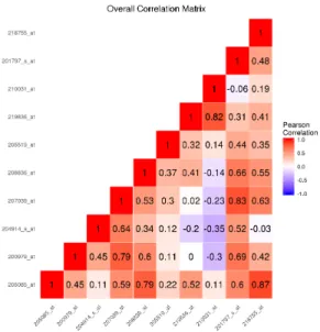
K = 3 classes. . . 4 2 The sample correlation matrix of the features simulated to be important to
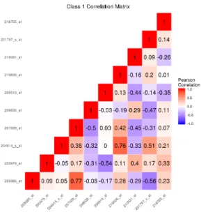
class separation for the linear decision boundary simulation with K = 3 classes. . 37 3 Among observations in class 1, the sample correlation matrix of the
fea-tures simulated to be important to class separation for the nonlinear decision
boundary simulation with K = 3 classes. . . 38 4 Among observations in class 2, the sample correlation matrix of the
fea-tures simulated to be important to class separation for the nonlinear decision
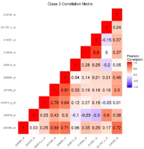
boundary simulation with K = 3 classes. . . 38 5 Among observations in class 3, the sample correlation matrix of the
fea-tures simulated to be important to class separation for the nonlinear decision
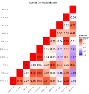
boundary simulation with K = 3 classes. . . 39 6 The sample correlation matrix of the features simulated to be important to
class separation for the linear decision boundary simulation with K = 4 classes. . 40 7 Among observations in class 1, the sample correlation matrix of the
fea-tures simulated to be important to class separation for the nonlinear decision
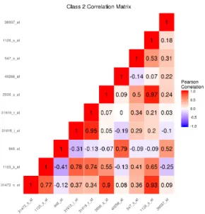
boundary simulation with K = 4 classes. . . 40 8 Among observations in class 2, the sample correlation matrix of the
fea-tures simulated to be important to class separation for the nonlinear decision
boundary simulation with K = 4 classes. . . 41 9 Among observations in class 3, the sample correlation matrix of the
fea-tures simulated to be important to class separation for the nonlinear decision
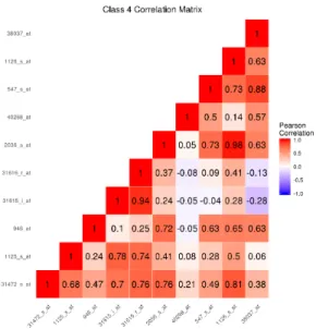
boundary simulation with K = 4 classes. . . 41 10 Among observations in class 4, the sample correlation matrix of the
fea-tures simulated to be important to class separation for the nonlinear decision
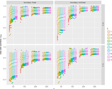
11 Test set Somers’ DXY for models fit using the binary aggregation approach
to the Ordinal FANS algorithm. As the number of classifiers in the FANS
ensemble (L) increases, the predictive performance improves monotonically. . . . 44 12 Test set Somers’ DXY for models fit using the boosting approach to the
Ordi-nal FANS algorithm. As the number of classifiers in the FANS ensemble (L)
increases, the predictive performance improves monotonically. . . 45 13 Test set Somers’ DXY for models fit using the Ordinal FANS binary
aggrega-tion approach (blue) and the Ordinal FANS boosting approach (red). Results
are presented for L= 10 FANS iterations. . . 45 14 Sensitivity for models fit using the Ordinal FANS binary aggregation approach
(blue) and the Ordinal FANS boosting approach (red). Results are presented
for L= 1 FANS iteration. . . 48 15 Specificity for models fit using the Ordinal FANS binary aggregation approach
(blue) and the Ordinal FANS boosting approach (red). Results are presented
for L= 1 FANS iteration. . . 49 16 10-fold cross-validation estimates of Somers’ DXY for the classification of
nor-mal, HSIL, and cervical carcinoma samples from GSE7803. Results are shown for the P/O boosting approach (red) and binary model aggregation approach
(blue). . . 49 17 10-fold cross-validation estimates of the misclassification rate for the
clas-sification of normal, HSIL, and cervical carcinoma samples from GSE7803. Results are shown for the P/O boosting approach (red) and binary model
aggregation approach (blue). . . 51 18 10-fold cross-validation estimates of the class-specific misclassification rates
for the classification of normal (red), HSIL (green), and cervical carcinoma (blue) samples from GSE7803. Results are shown for the P/O boosting
ap-proach (red) and binary model aggregation apap-proach (blue). . . 51 19 Simulation results: Distribution of test set Somers’ DXY estimates for varying
K, n, and decision boundaries for each method in the comparative analysis. . . . 64 20 Simulation results: Distribution of sensitivity for varying K, n, and decision
boundaries. . . 68 21 Simulation results: Distribution of specificity for varying K, n, and decision
22 Proportion missing among predictors with at least one missing value in the
AML dataset. . . 91 23 Proportion missing among samples with at least one missing value in the
AML dataset. . . 91 24 Validation set estimates of Somer’s DXY from the simulation study for models
fit using each of the four assumptions and for different proportions of censor-ing. Results from both the AIC-selected (red) and BIC-selected (blue) models
are shown. . . 95 25 The distribution of sensitivity estimates from the simulation study for models
fit using each of the four assumptions and for different proportions of censor-ing. Results from both the AIC-selected (red) and BIC-selected (blue) models
are shown. . . 97 26 The distribution of specificity estimates from the simulation study for models
fit using each of the four assumptions and for different proportions of censor-ing. Results from both the AIC-selected (red) and BIC-selected (blue) models
are shown. . . 98 27 Leave-one-out cross-validation estimates of Somer’s DXY ±one standard error
for models fit using the AML data and for each of the four assumptions. Results from both the AIC-selected (red) and BIC-selected (blue) models are
Abstract
METHODS FOR PREDICTING AN ORDINAL RESPONSE WITH HIGH-THROUGHPUT GENOMIC DATA
By Kyle L. Ferber
A dissertation submitted in partial fulfillment of the requirements for the degree of Doctor of Philosophy at Virginia Commonwealth University.
Virginia Commonwealth University, 2016. Major Director: Kellie J. Archer, Ph.D.,
Professor, Department of Biostatistics
Multigenic diagnostic and prognostic tools can be derived for ordinal clinical outcomes using data from high-throughput genomic experiments. For example, one may wish to classify tissue samples as healthy, pre-malignant, or malignant using data from a microarray experiment. Here, the goal is twofold: to develop an accurate classifier of the ordinal outcome and to select features that play an important role in the tissue’s progression from a healthy to a malignant state.
A challenge in this setting is that the number of predictors is much greater than the sample size, so traditional ordinal response modeling techniques must be exchanged for more specialized approaches. Existing methods perform well on some datasets, but there is room for improvement in terms of variable selection and predictive accuracy. Therefore, we extended an impressive binary response modeling technique, Feature Augmentation via Non-parametrics and Selection (FANS), to the ordinal response setting and developed software for implementing the extension. Through simulation studies and analyses of high-throughput genomic datasets, we showed that our Ordinal FANS method is sensitive and specific when discriminating between important and unimportant features from the high-dimensional fea-ture space and is highly competitive in terms of predictive accuracy.
Discrete survival time is another example of an ordinal response. For many illnesses and chronic conditions, it is impossible to record the precise date and time of disease onset or
relapse. Further, the HIPPA Privacy Rule prevents recording of protected health information which includes all elements of dates (except year), so in the absence of a “limited dataset”, date of diagnosis or date of death are not available for calculating overall survival. Therefore, increasingly survival is collected as a discrete event time. We previously demonstrated that a penalized forward continuation ratio model can be fit to discrete survival time data in high-dimensional settings, but this model does not incorporate censoring information. Thus, we developed a method that is suitable for modeling high-dimensional discrete survival time data while accommodating censoring information and assessed its performance by conducting a simulation study and by predicting the discrete survival times of acute myeloid leukemia patients using a high-dimensional dataset.
CHAPTER 1
INTRODUCTION
1.1 Motivation
Physicians are faced with difficult medical decisions on a daily basis. Oncologists, for instance, need to personalize treatment plans for their patients. If the desired results are not obtained after a given amount of time, they may need to consider switching therapies. These choices are made based on expert medical knowledge, intuition, and past experiences, and each decision they make will affect their patients’ survival times. Consequently, two independent, equally qualified physicians may make different decisions about what is best for the well-being of a patient. A more objective method for making certain medical decisions is to use data collected on past patients to build a predictive model that can be applied to future patients.
Consider the case of a breast cancer patient with three treatment options. The physician will choose one of the three options, the patient will be given that treatment, and then the physician will assess how well the treatment worked based on characteristics of the residual disease. The success of treatment can be measured using the residual cancer burden (RCB) index, an ordinal measure (RCB-I < RCB-II < RCB-III) that takes into account primary tumor bed dimensions, cellularity fraction of invasive cancer, size of largest metastasis, and the number of positive lymph nodes [1]. Alternatively, data on patients who have received each of the three treatments could be used to build a regression model. Then, the patient would be given whichever treatment the model predicted will result in the best outcome. In this situation, neither the physician nor the data-driven model are going to make the best decision 100% of the time. Ayers (2007) argues this by stating “In the end, super crunching is not a substitute for intuition, but rather a complement [2].” By super crunching, he is
referring to the practice of using large amounts of data to make informed decisions. He then goes on to say, “Traditional experts make better decisions when they are provided with the results of statistical prediction. Those who cling to the authority of traditional experts tend to embrace the idea of combining the two forms of ‘knowledge’ by giving the experts statistical support [2].” Our goal in developing methods for fitting predictive ordinal response models is not to replace a physicians decision making, but rather to support it with additional information. The methods we developed utilize high-dimensional genomic data to predict patient outcome, whereas physicians typically make decisions based on standards of care that are often developed by clinical knowledge, not rigorous analyses of experimental data.
Predictive ordinal response models could also help in simpler situations, such as de-termining the grade of a particular tumor, which is a relatively subjective procedure done by examining the microscopic cell appearance. Tumor grade is taken into account when deciding on a treatment regimen, so it is important to make an accurate assessment. Gene expression can be taken into account through a predictive model to improve the accuracy of a pathologist’s diagnosis [3].
1.2 Analysis of ordinal response data
An ordinal response is unique in that there is an intrinsic ordering to the possible values of the response, but the distance between these possible values, called classes, is unknown. For instance, the four stages of cancer are ordered (stage I is less severe than stage II; stage II is less severe than stage III, etc.), but we cannot objectively measure the quantitative difference in severity between each of the four stages. Thus, ordinal variables are somewhat of a hybrid between a nominal categorical variable and a continuous variable. Ordinal re-sponses are ubiquitous in biomedical data. For example, in cancer research, discrete survival time, tumor grade, and the degree of regional lymph node involvement are all ordinal mea-surements. Furthermore, the severity of many conditions, such as heart failure, Alzheimer’s
disease, and chronic kidney disease, are defined by an ordinal stage of disease [4, 5, 6].
1.2.1 Ordinal regression
Ignoring any aspect of the ordinal response results in a loss of information. For instance, modeling an ordinal outcome using multinomial logistic regression, given below, ignores the ordering of the classes.
log P(Yi =k|xi)
P(Yi =K|xi)
=β0k+xiβk, k = 1, ..., K −1
Givenppredictors, this model estimates a different set ofpcoefficients for each of the K−1 logistic regression models, and as a result, it is difficult to interpret and is not parsimonious. Another approach for modeling an ordinal response is to assign each class an integer rank (i.e. 1, 2, ..., K) and use traditional linear regression to model the response. However, this method makes the unrealistic assumption that the distances between adjacent ordinal classes are equal. Furthermore, assigning integer values to the ordinal classes is arbitrary. For example, one could instead assigneven integers to the ordinal classes (2, 4, ..., 2K). Finally, a linear regression model assumes that Y|X is normally distributed. This assumption will clearly fail when the response is ordinal because the response is discrete and predicted values are not restricted to be between 1 and K.
Proportional odds models are a class of models that are appropriate for modeling an ordinal outcome. Models in this class only estimate pcoefficient estimates by taking advan-tage of the ordered structure and making a simple assumption. For example, for observation
i= 1,2, ..., n, the cumulative logit model is given by: logP(Yi > k|xi)
P(Yi ≤k|xi)
=αk+xiβ, k= 1, ..., K−1
In the estimation procedure, a constraint is placed on the class-specific intercepts, or thresh-olds, such that α1 < α2 < ... < αK−1, which preserves the positivity of the class-specific
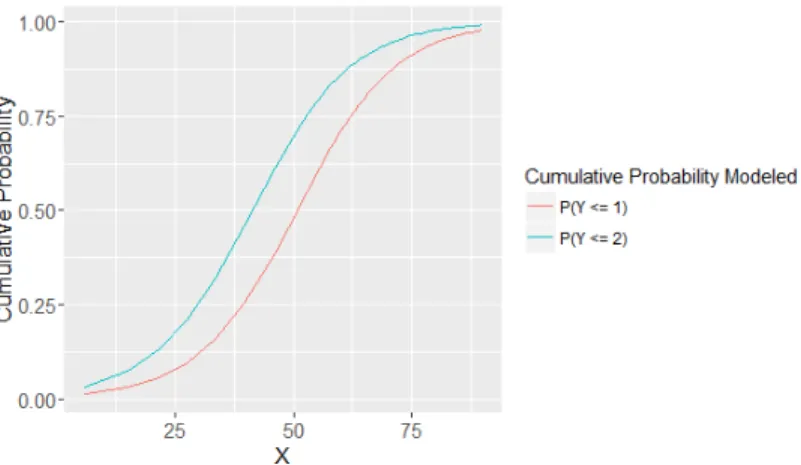
Fig. 1. A cumulative logit model with a single predictor and an ordinal outcome withK = 3 classes.
so K −1 parallel logit models are produced. Further, this model is a type of proportional odds model because the cumulative odds ratio is proportional to the difference between two vectors of predictors. The cumulative odds ratio, which is defined as the odds of Y > k
given X =x1 compared to the odds of Y > k given X =x2, is given by:
P(Y >k|x1) P(Y≤k|x1) P(Y >k|x2) P(Y≤k|x2) = exp(αk+x1β) exp(αk+x2β) = exp(αk+x1β−αk−x2β) = exp((x1−x2)β)
which does not depend on k. The proportional odds assumption is displayed by the parallel logistic curves in Figure 1.
Other logit-link proportional odds models include: • The adjacent category model:
logP(Yi =k+ 1|xi)
P(Yi =k|xi)
=αk+xiβ, k= 1, ..., K−1
• The backward continuation ratio model: logP(Yi =k|Yi ≤k,xi)
P(Yi < k|Yi ≤k,xi)
• The forward continuation ratio model: logP(Yi =k|Yi ≥k,xi)
P(Yi > k|Yi ≥k,xi)
=αk+xiβ, k = 1, ..., K −1
Furthermore, alternative link functions can be used for these models. For example, instead of the logit, the cumulative link model can utilize a:
• Probit link: Φ−1(P(Yi>k|xi)
P(Yi≤k|xi)) =αk+xiβ, where Φ is the cumulative distribution function
(CDF) of the standard normal distribution
• Complimentary log-log (cloglog) link: log(-log(1−P(Yi > k|xi))) =αk+xiβ
1.2.2 Maximum likelihood estimation
The length-nordinal response vectorycan be reformatted as annxK response matrix,
Y as follows, yik =
1 if observationi belongs to classk
0 otherwise
Then the log-likelihood can be expressed as [7]
L= n X i=1 K X k=1 yiklog[P(Yi =k|xi)]
Pratt (1981) and Burridge (1981) showed that the log-likelihoods of the cumulative link models are concave, so a unique global maximum exists [8, 9]. However, a closed-form solution does not exist, so an iterative algorithm is needed to find the maximum likelihood (ML) estimates of the parameters, β and α1, ..., αK−1. One such method that is commonly
used in low-dimensional problems (i.e. p < n) is the Newton-Raphson algorithm. Let the vector of all parameter estimates be denoted by θ = {α1, ..., αK−1, β1, ..., βp}. The gradient
of L, which consists of the partial derivatives of L with respect to each parameter, is given by g(θ) = (∂L ∂θ1 , ∂L ∂θ2 , ..., ∂L ∂θp+K−1 )
and the Hessian, the (p+K −1) x (p+K −1) matrix of second-order partial derivatives, is denoted by H(θ)= ∂2L ∂θa∂θb a,b∈{1,...,p+K−1}
Let the iteration number be denoted by s. The Newton-Raphson algorithm begins by spec-ifying starting values for the parameters that are to be estimated, θ[1]. The update at the next iteration and each of the subsequent iterations is
θ[s+1] =θ[s]−(H(θ[s]))−1g(θ[s])
The algorithm continues until convergence, which occurs when the difference between suc-cessive log-likelihoods, L(θ[s+1])−L(θ[s]), is negligible.
1.3 Microarray experiments
The central dogma of molecular biology states that the genetic information encoded in the DNA within the nucleus of each cell is transcribed into messenger RNA (mRNA), and the mRNA is then translated into proteins in the cell cytoplasm. Genes are the regions of DNA that encode instructions to produce proteins, and proteins are “used to support the cell structure, to break down chemicals, to build new chemicals, to transport items, and to regulate production [10].” Put simply, genes dictate which proteins and how much of the proteins should be synthesized, and proteins control cell function. Thus, along with environmental factors, genes determine the characteristics, or phenotypes, of cells and as a result, the entire organism [11]. Furthermore, aberrant cell function can lead to a host of diseases, so interest lies in detecting which genes are involved in causing the problem. We can measure the activity of a gene (calledgene expression) by quantifying the amount of mRNA that is transcribed from that particular gene. A microarray does this for thousands of genes simultaneously. There are many assays developed by different companies, but we analyzed data from two of the most common platforms, Affymetrix GeneChips and Illumina BeadChips. The technology involved in the two arrays is quite different, but the goal is
the same: to quantify the expression of the tens of thousands of genes present on the chip. Each gene is represented on the array by a set of short sequences of nucleotides called oligonucleotides. Each chip is used to measure a single patient’s gene expression. Thus, a typical experiment involves n microarrays and the goal is to detect differences in expression between groups with different phenotypes (e.g. cancer patients and healthy patients). There are a multitude of statistical challenges that arise from microarray experiments. The data are inherently noisy because there are many sources of obscuring variation, including from array fabrication and image processing [11]. However, we will be focusing on the statistical challenges that arise once the data has been cleaned and normalized: namely the fact that there are far more predictors than samples in a typical experiment, i.e. p >> n.
1.4 High-dimensional classification
Traditional methods for fitting classification and regression models require the number of subjects, n, to be larger than the number of predictors, p, and they assume that the predictors are independent. However, in high-throughput genomic experiments, we cannot safely assume independence of the predictors (often called features in this field) andp >> n, which results in a host of complexities. First, the design matrix will not be full-rank, which eliminates the ability to find a stable, unique solution. Second, with a large number of predictors relative to the sample size, a subset of the predictors is likely to exhibit collinearity, which will lead to unstable parameter estimates. Furthermore, genomic data is typically sparse, meaning out of the thousands of features, only a small proportion are associated with the response, which complicates the process of discovering significant features. Model building tools such as forward and backward stepwise selection are not feasible given the huge number of predictors.
1.4.1 Least Absolute Shrinkage and Selection Operator
Recently, penalization (also referred to as regularization) has stood out as an effective method to combat the issues that come with high-dimensional data. There are several popular penalization methods, but the defining characteristic of them all is that they shrink the absolute coefficient estimates towards 0. As a result, bias is introduced into the parameter estimates in exchange for a reduction in variance. In cases where model parsimony and interpretability are important, the least absolute shrinkage and selection operator (LASSO) penalization method is effective as it shrinks parameter estimates deemed unimportant to be exactly zero [12]. LASSO models are fit by maximizing the likelihood of the data minus a penalty term, as given below:
ˆ β = argmax β L(β|y,x)−λ P X p=1 |βp| !
The tuning parameter, λ, controls the balance between bias and variance. Traditional max-imum likelihood estimation occurs when λ = 0, but as previously mentioned, when p > n, there is no unique solution. Therefore, the parameter estimates will have minimal bias but will be highly unstable (high variance). As λ increases, the parameter estimates shrink to-wards 0. As this happens, more bias is added to the estimates, but the variance decreases. Asλ increases, the number of nonzero coefficient estimates decreases, which leads to a more stable and interpretable model.
Hastie et. al showed that the Generalized Monotone Incremental Forward Stagewise (GMIFS) algorithm solves for the LASSO solution in a penalized logistic regression model [13]. The algorithm proceeds as follows:
1. Enlarge the predictor space as ˜X = [X : −X] , where X represents the standardized predictors.
2. For step s=0, initialize the components of ˆβ(s) as ˆβ1 = ˆβ2 = ...= ˆβP = ˆβP+1 = ...=
ˆ
3. Find m = argmin
j
-δlogL/δβj at the current estimate ˆβ
(s)
.
4. Update ˆβm(s+1) = ˆβm(s)+, where is a small step size, such as 0.001.
5. Repeat steps 3 to 4 many times.
The design matrix is expanded with its negated version to avoid the computationally bur-densome step of calculating the second derivative, which would have been needed to find the step direction in step 4. The final coefficient estimates are given by
ˆ
βj = ˆβj −βˆj+P, j = 1, ..., p
The GMIFS method was extended by Archer et al. for fitting logit, probit, and complimen-tary log-log link ordinal response models (cumulative, adjacent category, stereotype, forward continuation ratio, and backward continuation ratio) to high-throughput genomic data[7]. We discuss this method in detail in Chapter 4.
1.4.2 Component-wise gradient boosting
Another method for fitting a logistic regression model in high-dimensional data settings is called componentwise gradient boosting [14]. According to Hastie et. al, boosting is “one of the most powerful learning ideas introduced in the last twenty years.”[15] It is one method in a class of ensemble schemes that combines multiple weak function estimates to form one aggregated estimator. The aim of boosting is to estimate a function, f∗(·), that minimizes the risk:
R=E[L(Y, f(X))],
whereLis the loss function chosen dependent on the structure of the response[14]. Gradient boosting searches for the solution by following the steepest path down the gradient of the empirical risk function, n1Pn
i=1L(yi, f(xi)) in function space. Gradient boosting can be
applied to many different estimators including regression trees, generalized linear models (GLMs), and Cox proportional hazards models, but we limit our discussion to GLMs. Most
often the loss function is the negative log-likelihood of the response distribution and f is assumed to belong to a parameterized class of functions, f(x,P). The component-wise gradient boosting algorithm for GLMs is as follow:
1. Center the predictors and set m= 0.
2. Initialize ˆβ[0] = 0, where ˆβ[0] is the vector of initial parameter estimates of length p. 3. Initialize the function estimate as ˆf[0] = argmin
c
Pn
i=1L(yi, c), where ˆf is a vector of
length n.
4. Increase m by 1 (m represents the number of iterations).
5. Compute the negative gradient of the loss function with respect to f and, for each observation, evaluate it at the estimate of the previous iteration, fˆ[m−1](xi):
U[m]=Ui[m] i=1,...,n = − δ δfL(yi, f)|f=fˆ[m−1](xi) i=1,...,n
6. Fit each predictor, xj, separately to the negative gradient vector U[m] using a “base learner,” h(xj;βj), j = 1, ..., p. A base learner in this context is a simple linear
model, and the coefficient in each model is estimated using least squares. Each of the
p models will result in a different estimate ofU[m].
7. Select the model that fits the negative gradient best as determined by the residual sum of squares criterion. Let ˆU[m] represent the vector of predicted values for that model and assign the estimated coefficient of that model to ˆβs.
8. Update the current function estimate and parameter estimate:
ˆ
f[m] =fˆ[m−1]+νUˆ[m] ˆ
β[m] =βˆ[m−1]+νβˆs
Note that ν is a pre-specified small step length factor between 0 and 1. Also, βˆ[m] is the vector of coefficient estimates, while ˆβs is a single coefficient estimate.
Repeat steps 4-8 until m = mstop, where mstop represents the stopping iteration which is
generally chosen by cross-validation or an information criterion. Furthermore, the choice of ν is not highly influential; any small value (e.g. ν = 0.1) is fine[14]. A cumulative logit ordinal response model can be fit using an extension of component-wise gradient called proportional odds boosting [16]. We will discuss this method in Chapter 2.
1.5 Measuring model performance
We are interested in assessing the models’ ability to accurately predict the outcome of new observations as well as their ability to discriminate between important and unimportant features in the high-dimensional feature space.
1.5.1 Prediction
To assess prediction in a classification setting with a binary outcome, the misclassifica-tion rate, which is defined as
#(Y 6= ˆY)
n
is often utilized. The misclassification rate is a useful and simple measure. However, in the ordinal response setting, the severity of the misclassifications is lost. For instance, the same penalty is applied if an observation in class 1 is classified to class 2 or to class 4. Therefore, a better method is to examine the misclassification rate separately for each class. The resulting
K measures are called the class-specific misclassification rates.
Another useful metric examines the association between the observed and predicted values in terms of discordance and concordance. Let ya and ˆya be the observed and the
predicted ordinal response variables, respectively, for subject a. Given a pair of subjects, if the subject that has a larger observed value also has the larger predicted value, the pair of subjects is concordant. If the subject that has a larger observed value has the smaller predicted value, the pair of subjects is discordant. Now, let C represent the number of concordant pairs in a sample and D represent the number of discordant pairs. Define TY
as the number of pairs in which the two subjects had the same observed response value (i.e. they were tied with respect to y). Somer’s D is an asymmetric measure of association, meaning we cannot treat the two variables interchangeably. We used Somer’s DXY, which
measures how wellX serves as a predictor ofY [17]. Here,X represents the predicted value, or ˆya, and Y represents the observed outcome, ya. The sample version of Somer’s DXY is given by:
DXY =
C−D n(n−1)/2−TY ,
where the numerator represents the difference in the number of concordant and discordant pairs, and the denominator represents the total number of pairs that are untied onY. DXY
ranges from -1 to 1, where DXY = −1 indicates a perfect negative association, DXY = 1 indicates a perfect positive association, and DXY = 0 indicates no association.
1.5.1.1 10-Fold cross-validation
One way of assessing performance is to fit a model to the entire dataset, predict the outcome of the observations in the same dataset, and then estimate the metrics described previously using the predictions. This method gives overly optimistic results and does not estimate how well the model’s performance will generalize to independent data. One way of overcoming these shortcomings is to use 10-fold cross-validation, which proceeds as follows:
1. Split the data evenly into 10 equal partitions. 2. For m = 1,2, ...,10:
(a) Fit a model using all partitions except partition m.
(b) Predict the outcome of observations in partition m using the fitted model. (c) Estimate the performance measure(s) using the predicted classes of observations
in partitionm.
3. Let nm denote the sample size of partition m, and let n denote the total sample size.
observations in partition m (e.g. Somers’ DXY). Estimate the 10-fold cross-validation
estimate of the metric, ˆw, as
ˆ w= 10 X m=1 nm n wˆm 1.5.2 Feature selection
Let the features that are truly associated with the ordinal response be deemed important, and we call the features that are not associated with the outcome unimportant. To assess feature selection in simulations, where we know which features are important and which are unimportant, we estimate
1. Sensitivity = Number of important features selectedTotal number of important features
2. Specificity = Number of unimportant featuresTotal number of unimportant featuresnot selected
In gene expression data analyses when we do not know which features are truly impor-tant and which are truly unimporimpor-tant, we can examine the features selected by the model in the literature in an attempt to validate model findings.
1.6 Discussion
In this chapter, we have provided the necessary overview of ordinal regression as well as methods for fitting penalized classification and regression models. In Chapter 2, we introduce the method we developed, Ordinal Feature Augmentation via Nonparametrics and Selection (FANS). This method is compared to other methods suitable for fitting high-dimensional ordinal response models in Chapter 3. To that end, we examine prediction accuracy as well as feature selection in a simulation study and several gene expression data analyses. Next, in Chapter 4, a novel method for performing discrete time survival analysis in high-dimensions is described. Finally, we conclude with a discussion of the methods developed as well as future work in Chapter 5.
CHAPTER 2
FEATURE AUGMENTATION VIA NONPARAMETRICS AND SELECTION
2.1 Introduction
2.1.1 Ensemble learners
In a supervised learning problem with a discrete outcome, the goal is to use a training sample of known outcomes and predictors, {yi,xi}n1, to build a classifier that accurately
predicts the outcome of a future observation. An ensemble learner is composed of two or more classifiers, with the idea that the combination of classifiers should produce more accurate predictions than any of the individual models. However, the constituents must be both accurate and diverse in order for an ensemble to be more accurate than any of the individual classifiers [18]. Here, an accurate classifier is defined as one with a misclassification rate lower than that of random guessing, and two classifiers are said to be diverse if they make different errors on new data [19]. In the ordinal response setting, the misclassification rate of random guessing is equal to KK−1, where K denotes the number of classes in the outcome.
There are several methods for constructing an ensemble learner that can be applied to a variety of classification and regression algorithms [19]. One method forms an ensemble of classifiers using manipulated versions of the training data. Breiman (1994) created one of the first ensemble schemes in this way [20]. The method, called bootstrap aggregation, or bagging for short, generates multipledecision trees using bootstrap replicates of the training data. To build a decision tree, all observations begin together in one set, called a root node. The observations are then partitioned, or split, into two distinct sets, called nodes. Each of these nodes is then further split into two nodes. This process continues until some stopping criteria is met. At each step, to determine the optimal split, we need a set of binary questions
which are defined such that [21]:
1. Each split depends on only one predictor.
2. For ordered (ordinal and continuous) predictors, the question takes the form, “Is x≤
c?”, where cis in the set of observed values for that predictor.
3. For nominal predictors, the binary question takes the form, “Is x∈ A?, where A is a subset of the observed values for that predictor.
Bagging begins by sampling n observations with replacement from the training data of size n to create abootstrap replicate. Then, a classifier is built using the bootstrap replicate. This procedure of sampling with replacement from the training data and then building a classifier using the bootstrap replicate is repeated many times. When the outcome is discrete, the classifiers are aggregated by plurality voting. That is, each classifier returns a prediction for a new observation, and the class with the most “votes” is the predicted class [20]. The performance of the ensemble generally improves as the number of constituent classifiers increases. However, at a certain point, the performance stabilizes and adding more classifiers does not help much. With bagging, Breiman succinctly states that “what one loses...is a simple and interpretable structure. What one gains is increased accuracy.”[20] Manipulating the input features is another method for constructing an ensemble [19]. For instance, Cherkauer (1996) trained an ensemble of 32 models based on 8 different sub-sets of the 119 available features and 4 different tuning parameters [22]. This method for constructing an ensemble only works well when the predictors suffer from collinearity [19].
A third technique for building an ensemble learner is to manipulate the outcome variable. A method called error-correcting output coding randomly partitions the K classes of a discrete (nominal) outcome into two subsets, A and B [23]. The training data are re-coded so that the outcome for all observations whose response is inAis coded as 0 and the outcome for any observations whose response is in B is coded as 1. Then, a classifier is built using the binary outcome. The steps of partitioning the outcome classes, re-coding the multi-class
outcome for each observation in the training data, and then fitting a binary response model is repeatedLtimes. For a new observation, each of theL classifiers will predict whether the outcome is in AorB. Each time a classifier predicts the outcome is inA, the classes in that subset receive a vote, and likewise for subset B. Then, the class with the most votes is the predicted class on the original multi-class scale [23].
Finally, a fourth general method for building an ensemble of classifiers is to inject randomness into the learning algorithm [19]. Random forest is one of the most common ensemble schemes and it improves on bagging by injecting randomness into the tree building procedure [24]. At each step in the tree-building procedure, instead of considering all features when searching for the best split, random forest considers a random subset of the features. This helps to reduce the correlation among the classifiers (trees) that are aggregated, which drives down the variance of the ensemble learner.
2.1.2 Feature Augmentation via Nonparametrics and Selection
Feature Augmentation via Nonparametrics and Selection (FANS) is a two-class modeling procedure that has shown promising results in high-dimensional learning problems [25] by building an ensemble of classifiers in a unique way. Suppose we have n feature-outcome pairs in a training set, T ={(xi, yi)}
n
i, where yi ∈ {0,1} and xi ∈Rp. We begin with some
definitions. Let g(x) = P(X = x|Y = 0), f(x) = P(X = x|Y = 1), and π = P(Y = 1). The Bayes classifier, which minimizes the probability of misclassifying an observation, assigns observations to class 1 if P(Y = 1|X) > 0.5 and to class 0 otherwise. Thus, the Bayes-optimal decision boundary is defined as
{x:P(Y = 1|x) =P(Y = 0|x)} ⇒ {x: πf(x) πf(x) + (1−π)g(x) = (1−π)g(x) πf(x) + (1−π)g(x)} ⇒ {x: πf(x) (1−π)g(x) = 1}
If we assume equal priors, i.e. P(Y = 1) = P(Y = 0), then the Bayes decision boundary becomes {x: f(x) g(x) = 1}={x: log f(x) g(x) = 0}.
Thus, given a single feature, x, the best univariable classifier of y is [25]
ˆ y= 1 if logfg((xx))>0 0 if logfg((xx))<0
The Na¨ıve Bayes classifier assumes the p features within each class are independent, so the joint distribution of features in the two classes becomes f(x) = Qp
j=1fj(xj) and
g(x) =Qp
j=1gj(xj). Consequently, the nonparametric Na¨ıve Bayes decision boundary is
( x: p X j=1 logfj(xj) gj(xj) = 0 ) .
However, this independence assumption is too strong in most cases. For example, in a gene expression microarray experiment, each feature is designed to interrogate a gene (or part of a gene), and we know that genes interact in biological networks. Hence, non-zero correlations exist among some sets of genes. Thus, assuming the features from a microarray experiment are independent would be ill-advised. The FANS method attempts to account for dependence among the features by adding optimized weights to the Na¨ıve Bayes classifier to form the following decision boundary [25]:
FANSD = ( x:β0+ p X j=1 βjlog fj(xj) gj(xj) = 0 ) .
The method combines the best univariable predictors in a linear and additive manner in an attempt to create a powerful multivariable classifier. Note that the decision boundary based on the original features is nonlinear, which makes the classifier more flexible. However, since FANSD is linear in the coefficients, we can rename the transformed variables (i.e. zj =
logfj(xj)
gj(xj)) and apply any binary linear classification procedure to estimate the coefficients. When p > n, the model is overparameterized, so penalization/regularization techniques are
required to fit the model. These methods shrink the coefficient estimates towards zero, which adds bias in exchange for a reduction in variance, leading to improved model performance [15]. The FANS classifier uses penalized logistic regression [25] and is fit using the following algorithm that utilizes data splitting and prediction averaging to build an ensemble learner [25]:
1. Randomly partition the data into two sets, (D1, Dc1), analogous to splitting data into
a training set and a test set.
2. UsingD1, estimatefj(xj) =P(Xj =xj|Y = 1) and gj(xj) =P(Xj =xj|Y = 0), j =
1, ..., p by kernel density estimation. Denote the estimates as ˆf = ( ˆf1, ...,fˆp) and
ˆ
g= (ˆg1, ...,ˆgp).
3. Use the data in Dc
1 to calculate the matrix of transformed variables, Z, where
zij = log " ˆ fj(xij) ˆ gj(xij) # , xij ∈D1c 4. Using Z and y ∈Dc
1, fit an L1 penalized logistic regression model.
5. Repeat steps 1-4 L times to obtain (D1, D1c), ...,(DL, DcL). However, the partitions in
step 1 are formed differently for odd and even numbered iterations. For odd numbered iterations, the training set is randomly partitioned. For even numbered iterations, the roles of the partitions in the preceding odd numbered iteration are reversed. That is, the first partition estimates the marginal densities for odd numbered iterations, but for even numbered iterations, the second partition estimates the marginal densities. In general, (D2l, Dc2l) = (D2cl−1, D2l−1) forl = 1, ...,bL2c, where (D2l−1, D2cl−1) is formed by
randomly partitioning T and (D2l, D2cl) is formed by reversing the roles of D2l−1 and
Dc
2l−1.
In order to predict the outcome of a new observation, xi = (xi1, ..., xip), we must use
obtain a different estimate of f and g, and a different fitted model. Thus, for each of the
l = 1,2, ..., Lpartitions, we can use ˆfl and ˆgl to transformxi and obtainzil = (zi1l, ..., zipl),
where zijl = log " ˆ fjl(xij) ˆ gjl(xij) # , j = 1, ..., p.
So, we end up with L vectors of transformed features, one from each iteration of the FANS algorithm. Each one can be input into the corresponding fitted model from step 4 in order to obtain a predicted probability, pil = ˆP(Yi = 1|zil). The average of these L
predicted probabilities, ¯pi = L1 PL
l=1pil, is used to classify the observation according to the
Bayes classifier: if ¯pi >0.5, predict class 1; otherwise, predict class 0 [25].
In step one, the roles of the data used for the density estimation and model fitting are reversed from one partition to the next in order to ensure a balanced assignment of data for the two tasks [25]. Partitioning the data multiple (L) times and averaging the predicted probabilities makes efficient use of the data and ensures the procedure is robust to arbitrary assignment of data to the two tasks [25].
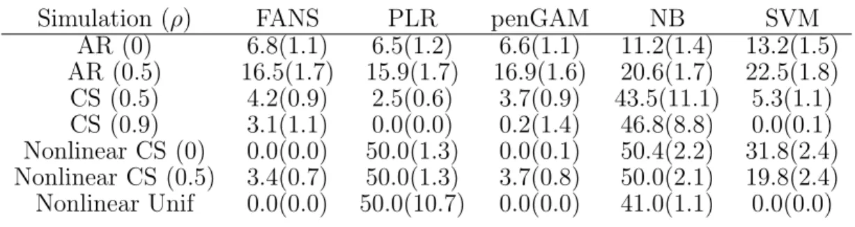
Several simulation examples were reported in the FANS manuscript [25]. The first three simulations generated the features in each class from a multivariate Gaussian distribution. The first let the two classes be linearly separable with an autoregressive (1) correlation structure among the features. The second simulation was the same as the first except the correlation structure was changed to be compound symmetric. The third generated the two classes to be separable by a nonlinear decision boundary with a compound symmetric correlation structure. Finally, the fourth simulation used a nonlinear decision boundary but generated the features using a uniform distribution. The FANS method performed as well or better than the competing methods including penalized logistic regression (PLR), penalized additive logistic regression (penGAM), Na¨ıve Bayes (NB), and support vector machines (SVM) (Table 1) [25]. The most competitive method to FANS in terms of misclassification error was penGAM. However, the median computation time for the simulations ranged from 3.4 to 6.6 seconds for FANS and 243.7 to 4811.9 seconds for penGAM, so FANS seemed to
Table 1. Median classification error (%) on an independent test set with standard errors for the simulation study. Different values of ρwere used for each example.
Simulation (ρ) FANS PLR penGAM NB SVM
AR (0) 6.8(1.1) 6.5(1.2) 6.6(1.1) 11.2(1.4) 13.2(1.5) AR (0.5) 16.5(1.7) 15.9(1.7) 16.9(1.6) 20.6(1.7) 22.5(1.8) CS (0.5) 4.2(0.9) 2.5(0.6) 3.7(0.9) 43.5(11.1) 5.3(1.1) CS (0.9) 3.1(1.1) 0.0(0.0) 0.2(1.4) 46.8(8.8) 0.0(0.1) Nonlinear CS (0) 0.0(0.0) 50.0(1.3) 0.0(0.1) 50.4(2.2) 31.8(2.4) Nonlinear CS (0.5) 3.4(0.7) 50.0(1.3) 3.7(0.8) 50.0(2.1) 19.8(2.4) Nonlinear Unif 0.0(0.0) 50.0(10.7) 0.0(0.0) 41.0(1.1) 0.0(0.0) be much more computationally efficient [25].
The authors also compared the predictive performance of FANS and the other methods using a lung cancer gene expression dataset. There were p = 12,533 features and n = 181 observations, where the number of observations in the training set, ntrain, was 32, and the
number of observations in the test set, ntest, was 149. The aim was to predict whether
observations in the test set were adenocarcinoma (ADCA) or mesothelioma [25]. With
L = 20 partitions, FANS obtained a 0% misclassification rate, while the other methods failed to do so [25].
In order to independently verify the predictive performance of FANS, we coded the method in the R programming environment [26] and compared the performance of models fit using FANS, penalized logistic regression, and Na¨ıve Bayes. We applied the three methods to a publicly available lung cancer gene expression dataset, GSE4115, where there were
n = 163 observations after removing samples without a definitive cancer diagnosis and
p = 22,215 features [27]. We split the data into a training set and an independent test set. Given the fact that the training set is partitioned into two sets in the first step of the FANS algorithm, we wanted to ensure there was enough data in the first set to estimate the marginal densities. Therefore, we assigned 23 of the data to the training set (ntrain = 136)
and the remaining 13 to the test set (ntest = 27). For the FANS model, we set L = 2, 10,
and 20. The aim was to predict whether subjects had lung cancer or not [27]. The model fit using FANS with L = 20 achieved a 0% misclassification rate on the independent test set,
while the misclassication rates for the penalized logistic regression and Na¨ıve Bayes models were 25.9% and 18.5%, respectively. Therefore, we also identified FANS as a competitive algorithm in the binary response case. With L = 2 and L = 10, the FANS misclassication rates were 14.8% and 3.7% respectively, suggesting that the data splitting and prediction averaging scheme in the FANS algorithm is effective. For L = 2, 10, and 20, the runtime for FANS was 31.29 minutes, 114.63 minutes, and 312.09 minutes, respectively. Meanwhile, the runtimes for Na¨ıve Bayes and penalized logistic regression were 0.96 minutes and 0.293 minutes, respectively. However, we did not apply parallel programming techniques when we coded the FANS algorithm, which would have significantly reduced the runtime.
2.1.3 Extending FANS to the ordinal response setting
In the binary response setting, FANS models the class-conditional marginal density ratios, zj = log P(Xj =xj|Y = 1) P(Xj =xj|Y = 0) = logfj(xj) gj(xj) .
Because there are K >2 ordinal outcome classes, the augmented features must be redefined in the FANS algorithm to accommodate all K class-conditional density estimates. One approach to create the ordinal augmented features is to consider the decision boundaries between adjacent classes, which would result in K−1 augmented features for each original feature: zj(1) = log " ˆ P(Xj =xj|Y = 1) ˆ P(Xj =xj|Y = 2) # zj(2) = log " ˆ P(Xj =xj|Y = 2) ˆ P(Xj =xj|Y = 3) # .. . z(jK−1) = log " ˆ P(Xj =xj|Y =K−1) ˆ P(Xj =xj|Y =K) # .
This approach reduces to the binary FANS method when K = 2. However, one issue is that the augmented features do not use the whole training set. Furthermore, the density estimates may be poor if there is not a sufficient number of observations in each class. Thus, the augmented features will be defined in a way that avoids these issues:
z(1)j = log " ˆ P(Xj =xj|Y = 1) ˆ P(Xj =xj|Y >1) # = log " ˆ fj(1)(xj) ˆ g(1)j (xj) # z(2)j = log " ˆ P(Xj =xj|Y ≤2) ˆ P(Xj =xj|Y >2) # = log " ˆ fj(2)(xj) ˆ g(2)j (xj) # .. . zj(K−1) = log " ˆ P(Xj =xj|Y ≤K −1) ˆ P(Xj =xj|Y =K) # = log " ˆ fj(K−1)(xj) ˆ gj(K−1)(xj) # . (2.1)
This way, each augmented feature uses the entire dataset, and the only densities that are class-specific (i.e. conditional on only one class) are ˆfj(1) and ˆgj(K−1). Furthermore, this approach also reduces to the binary FANS method when K = 2.
Now, because there are K −1 augmented features for each original feature, we must discover the best way to model the augmented features. One method is to include allK−1 in the model, resulting in (K − 1)∗ p input variables for the Ordinal FANS model. A typical Affymetrix HG-U133A microarray contains around 22,215 features, and if K = 4, we would need to model 22,215∗3 = 66,645 augmented features. This approach would greatly increase the computational time of fitting the model and may reduce the predictive accuracy of the model by increasing the sparsity of the solution. Another option would be to perform principal components analysis (PCA) on each of the p sets of K−1 augmented features. We could then fit a model with the first principal component (PC) from each analysis. However, if the first PC in each of the p PCAs does not explain the vast majority of the total variance, we would lose significant information by excluding the other PC’s. Therefore, we implemented two approaches:
1. Fit a penalized binary response model for each of the K−1 augmented features and aggregate the results using the technique proposed in the Ordinal Real AdaBoost algorithm [28]. We refer to this approach as the binary aggregation approach.
2. Fit a cumulative logit model using proportional odds boosting [16], where the K −1 augmented features for each predictor will either all be included or all be excluded from the fitted model. We refer to this approach as the boosting approach.
2.2 Approach 1: Aggregating penalized binary response models
Define the matrix, Z(k), which contains the elements z(k)
ij for subjects i ∈ {1,2, ..., n}
and featuresj ∈ {1,2, ..., p}. In other words,Z(k)is the design matrix for augmented feature
k, and z(ik) is a 1 xp row in Z(k). We will fit the following K −1 binary response models using Z(1), ...,Z(K−1): log P(Y = 1|z(1)) P(Y >1|z(1)) =β0(1)+z(1)β(1) log P(Y ≤2|z(2)) P(Y >2|z(2)) =β0(2)+z(2)β(2) .. . log P(Y ≤K −1|z(K−1)) P(Y =K|z(K−1)) =β0(K−1)+z(K−1)β(K−1) (2.2)
Each model is fit using L1-penalized logistic regression, which estimates the penalized solution given by ˆ β= argmax β L(β|y,z)−λ P X p=1 |βp| !
The resulting solution is sparse, meaning that the model fitting algorithm shrinks the coef-ficient estimates of features deemed unimportant to zero resulting in a parsimonious set of features with non-zero coefficient estimates. Thus, model fitting and feature selection are performed simultaneously. The tuning parameter,λ, controls the amount of shrinkage and is either chosen by cross-validation or by minimizing an information criterion (e.g. AIC, BIC).
Asλincreases, the number of parameter estimates that will be shrunk to zero also increases. The log-likelihood, L, of the kth logistic regression model is given by
L(β) = n X i=1 {I(Yi ≤k)log(P(Yi ≤k)|z(k)) +I(Yi > k)log(P(Yi > k)|z(k))} From equation (2.2), P(Yi ≤k)|z (k) i ) = exp{zi(k)β(k)} 1 + exp{zi(k)β(k)} P(Yi > k)|z (k) i ) = 1 1 + exp{zi(k)β(k)}
The binary response model fit using Z(k) will predict whether y ≤ k or y > k. For a
given subject i, define [28] ˆ p(1ki)= ˆp(2ki)=...= ˆp(kik)= ˆP(Yi ≤k|z (k) i ) ˆ p((kk)+1)i = ˆp((kk)+2)i =...= ˆp(Kik)= 1−Pˆ(Yi ≤k|z (k) i ).
For a given subjecti, each of theK−1 binary classifiers returns a vector, resulting in K−1 length-K vectors: (ˆp(1)1i ,pˆ(1)2i , ...,pˆ(1)Ki) (ˆp(2)1i ,pˆ(2)2i , ...,pˆ(2)Ki) .. . (ˆp(1Ki −1),pˆ2(Ki −1), ...,pˆ(KiK−1)) (2.3)
We can then sum the vectors from the binary classifiers fit usingZ(1), ...,Z(K−1) to form an aggregated vector of scores. The class with the largest score is the predicted class for that subject [28]: ˆ yi = argmax m K−1 X k=1 ˆ p(mik) (2.4)
1. Randomly partition the n feature-outcome pairs into two sets, (D1, D1c). 2. Using D1, estimate ˆf (1) j (xj), ...,fˆ (K−1) j (xj) and ˆg (1) j (xj), ...,ˆg (K−1) j (xj) for j = 1, ..., p
using kernel density estimation.
3. Evaluate the density estimates at the observed values inD1c, and calculate the matrices of augmented features, Z(1), ...,Z(K−1), where z(k)
ij = log ˆ fj(k)(xij) ˆ gj(k)(xij) ∈ Z(k) for x ij ∈ Dc 1, i= 1, ..., n and j = 1, ..., p and k= 1, ..., K−1. 4. Use y ∈ Dc
1 to fit the K − 1 binary classifiers defined in equation (2.2) using
L1-penalized logistic regression. The tuning parameter, λ is chosen by minimizing the AIC.
5. Reverse the roles of D1 and D1c and repeat steps 2 - 4. Let D2 =Dc1 and D2c=D1 .
6. Repeat steps 1 - 6 L
2 times, which results in L∗(K−1) penalized logistic regression
models based on the Ldifferent partitions, (D1, D1c), ...,(DL, DLc). 2.2.1 Predicting new observations
In order to predict the outcome of a new observation, x= (x1, x2, ..., xp), we must use
the densities and models estimated from the learning set. For each of the L partitions, we obtain different kernel density estimates and as a result, different fitted models. Thus, for each of theL partitions, we can use the kernel density estimates to transform xand obtain theK−1 length-pvectors of augmented features. Then, the augmented features are plugged into the respective fitted binary classifiers. Finally, the L∗(K−1) binary response models are aggregated to arrive at the class prediction on the ordinal scales.
Explicitly, for a new observation, x= (x1, x2, ..., xp),
1. Using the kernel densities estimated with D1, calculate ˆf (1) j (xj), ...,fˆ (K−1) j (xj) and ˆ gj(1)(xj), ...,ˆg (K−1) j (xj) for j = 1, ..., p.
2. Form the K−1 vectors augmented features, z(1)= log " ˆ fj(1)(xj) ˆ gj(1)(xj) # , j = 1,2, ..., p z(2)= log " ˆ fj(2)(xj) ˆ gj(2)(xj) # , j = 1,2, ..., p .. . z(K−1)= log " ˆ fj(K−1)(xj) ˆ gj(K−1)(xj) # , j = 1,2, ..., p
3. Plug each of the length-p vectors of augmented features into the respective fitted penalized logistic regression models in equation (2.2) and obtain the estimates of
P(Y ≤k|z(k)),k = 1,2, ..., K −1.
4. Form the vectors in equation (2.3). 5. Repeat 1-4 for (D2, D2c), ...,(DL, DcL).
6. Sum the L∗(K −1) vectors of scores. The element in the vector of sums with the largest value is the predicted value on the original ordinal scale,
ˆ y = argmax m L X l=1 K−1 X k=1 ˆ p(mk) 2.2.2 Feature selection
In addition to developing an accurate predictive model, we are interested in discriminat-ing between important and unimportant features from the high-dimensional set of predictors. This can be accomplished by running the FANS algorithm once, i.e. by setting L = 1. In this approach, the K −1 L1-penalized logistic regression models in equation (2.2) are fit, and each model produces a parsimonious set of features with non-zero coefficient estimates. The union of these sets is the final set of features selected.
2.3 Approach 2: Proportional Odds Boosting 2.3.1 Functional gradient descent
In the following setting, let y represent an outcome variable and let x = {x1, ..., xp}
represent a vector of p predictors. Recall that in a predictive learning problem, the goal is to use a training sample of known outcomes and predictors,{yi,xi}n1, to estimate a function
that maps x to y. The true, unknown function is denoted F∗(x) and the estimate is ˆF(x). Ideally, the function would be estimated by minimizing the expected value of a loss function (chosen depending on the distribution of y),Ey[L(y, F(x))|x] [29]. Minimizing the expected
loss (also known as the risk) in function space requires treating the functionF(x) evaluated at each x as a parameter. However, there is an infinite number of such parameters in Rp. If we instead attempt to simplify the estimation by using data, we can evaluate F at each
xi in the training set. Unfortunately, this approach breaks down because the expected loss cannot be estimated accurately using a finite dataset, and even if it could, estimates ofF∗(x) outside of the training set could not be obtained [29]. To remedy this situation, the function can be assumed to take a parametric form, F(x;P), where P ={P1, P2, ...} is a finite set
of parameters [29]. In this case, the function estimation problem can be simplified to one of parameter estimation. Boosting assumes an additive form for the function, given by
F(x;{νm,βm} M 1 ) = M X m=1 νmh(x;βm).
In this form, the base learner, h(x;β), is a simple function of the predictors (or a subset of the predictors), parameterized by β, and ν is a weight, or step size, for h. Futhermore, M
is the number of base learners that are combined to form the estimated function. The goal then becomes to estimate the parameters that minimize the empirical risk,
argmin {νm,βm}M1 n X i=1 L yi, M X m=1 νmh(xi;βm) ! .
In many problems, including when p >> n, this is infeasible, so a “greedy stagewise” ap-proach is taken [29]. For m= 1,2, ..., M,
1. (νm,βm) = argmin ν,β
Pn
i=1L(yi, Fm−1(xi) +νh(xi;β))
2. Fm(x) =Fm−1(x) +νmh(x;βm)
Here, νmh(x;βm) is called a step, where νm is the step size, and the vector h(x;βm) is the step direction. The goal is to take the largest possible step in the direction of the minimum of the empirical risk. By construction, the best steepest-descent step direction is the negative gradient evaluated at the prior step’s function estimates,
−gm(xi) =− ∂ ∂F(xi) L(yi, F(xi)) F(xi)=Fm−1(xi)
for x1, ...,xn, which is given by gm(x) = {−gm(xi)}ni=1. However, this gradient is only
defined at x1, ...,xn [29]. To generalize to other points outside the training set, we can
choose the base learner, h(xi;βm) that is most correlated with gm(x). This corresponds
to replacing the difficult two-step function estimation problem given above with a simple least squares estimation problem to choose the base learner, h, among a set of candidate base learners. Specifically, the negative gradient vector is fit using each base learner, and h
is set to the base learner with the smallest residual sum of squares (RSS). Then, Freidman states that we can use a line search to estimate νm [29], but B¨uhlmann and Hothorn have
suggested that the additional line search is unnecessary [14]. Using empirical evidence, they determined that one can simply use a single small constant step size ν, and further, the choice of ν is unimportant, as long as it is sufficiently small (such as 0.1) [14]. Thus, the generic boosting algorithm, without the line search for step size, is given by [29, 14]:
1. Specify a set of candidate base learners. These can be, for example, regression trees or linear models with a subset of the p predictors. Herein we focus our attention on linear models. The simplest setting specifies p base learners, where each base learner is a simple linear regression model with one of the p predictors as the sole input. For
example, the base learner for the jth predictor would be defined as gm(x) = xjβ+
2. Let m= 0 and initialize the vector of the estimated function evaluated at the n data points as F0(x) = argmin
c
Pn
i=1L(yi, c). That is, each element in the length-n vector
is initialized to the constant that minimizes the empirical risk. 3. Increase m by one and compute the negative gradient vector, gm(x).
4. Fit the negative gradient vector using each base learner. An estimate of the negative gradient vector is obtained from each fitted model. Denote the estimate from the base learner with the smallest RSS as ˆgm(x).
5. Update the function estimate, Fm(x) =Fm−1(x) +νgˆm(x;β).
6. Iterate steps 3-5 M times, whereM is a tuning parameter that is generally chosen by cross-validation [30].
Thus, the final function estimate takes the formF(x) =F0(x) +PMm=1νgˆm(x). 2.3.1.1 Proportional Odds Boosting
A cumulative logit proportional odds model for ordinal response data is given by
P(Y ≤k|x) = 1
1 + exp(F(x)−θk)
, k = 1, ..., K −1,
where F(x) is the prediction function defined in the previous section and {θ1, ..., θK−1} are
class-specific intercepts, or thresholds, that are constrained to be increasing from θ1 to θK
and are estimated simultaneously with F. The model can be expressed equivalently as log P(Y > k|x) P(Y ≤k|x) =F(x)−θk, k= 1, ..., K−1.
Using the given model, the class-specific probabilities can be estimated as: P(Y =k|x) =πk = 1 1+exp(F(x)−θ1) for k = 1 1 1+exp(F(x)−θk) − 1 1+exp(F(x)−θk−1) for 1< k < K 1− 1 1+exp(F(x)−θK−1) for k =K, (2.5)
which are used to specify the log-likelihood [16]:
l(F,θ) = −I(Y = 1)∗log[1 + exp(F(x)−θ1)]
+ K−1 X k=2 I(Y =k)∗log (1 + exp(F(x)−θk))−1−(1 + exp(F(x)−θk−1))−1 +I(Y =K)∗log 1−(1 + exp(f −θK−1))−1
Schmid et al. extended the generic boosting algorithm to the ordinal response setting, using the negative log-likelihood as the loss function, L, which resulted in the proportional odds (P/O) boosting algorithm [16]:
1. Let ˆFm and θˆm denote the vectors of estimates, ( ˆF(x1), ...,Fˆ(xn)) and (ˆθ1, ...,θˆK−1)
at step m. Set m= 0 and initialize ˆF0 and θˆ0.
2. Specify the base learners.
3. Increasemby 1 and compute the negative gradient of the loss with respect toF and, for each observation, evaluate it at the estimates of the previous iteration, ˆFm−1(xi),θˆm−1:
gm(x) = (−gm(xi))i=1,...,n = − δ δFL(yi, F,θ)|F= ˆFm−1(xi),θ=θˆm−1 i=1,...,n
4. Fit each of the base learners to the negative gradient vectorgm(x). Each model results in a different estimate of gm(x).
5. Select the model that fit the negative gradient best as determined by the R2
6. Update the current function estimate : ˆ
Fm = ˆFm−1 +νgˆm(x)
Note thatν is a pre-specified small step length factor between 0 and 1 and is not highly influential as long as it is sufficiently small (e.g. ν= 0.1) [14].
7. Treating the function estimate as fixed, estimate θm by minimizing the empirical risk,
1
n Pn
i=1L(yi,Fˆm,θ).
8. Repeat steps 3-7 until m =M, where M represents the stopping iteration chosen by cross-validation.
The final function estimate is given by ˆ FM = M X m=0 ˆ Fm = ˆF0+ M X m=1 νgˆm(x)
2.3.2 Fitting the Ordinal FANS model with Proportional Odds Boosting
We can model the augmented features i