University of Louisville University of Louisville
ThinkIR: The University of Louisville's Institutional Repository
ThinkIR: The University of Louisville's Institutional Repository
Electronic Theses and Dissertations8-2017
Accurate and justifiable : new algorithms for explainable
Accurate and justifiable : new algorithms for explainable
recommendations.
recommendations.
Behnoush AbdollahiUniversity of Louisville
Follow this and additional works at: https://ir.library.louisville.edu/etd
Part of the Artificial Intelligence and Robotics Commons, and the Other Computer Sciences Commons
Recommended Citation Recommended Citation
Abdollahi, Behnoush, "Accurate and justifiable : new algorithms for explainable recommendations." (2017). Electronic Theses and Dissertations. Paper 2744.
https://doi.org/10.18297/etd/2744
This Doctoral Dissertation is brought to you for free and open access by ThinkIR: The University of Louisville's Institutional Repository. It has been accepted for inclusion in Electronic Theses and Dissertations by an authorized administrator of ThinkIR: The University of Louisville's Institutional Repository. This title appears here courtesy of the author, who has retained all other copyrights. For more information, please contact [email protected].
ACCURATE AND JUSTIFIABLE: NEW ALGORITHMS FOR EXPLAINABLE RECOMMENDATIONS
By
Behnoush Abdollahi
M.Sc., Computer Engineering and Computer Science, University of Louisville, Louisville, KY
A Dissertation
Submitted to the Faculty of the
J.B. Speed School of Engineering of the University of Louisville in Partial Fulfillment of the Requirements
for the Degree of
Doctor of Philosophy in Computer Science and Engineering
Department of Computer Engineering and Computer Science University of Louisville
Louisville, Kentucky
Copyright 2017 by Behnoush Abdollahi
ACCURATE AND JUSTIFIABLE: NEW ALGORITHMS FOR EXPLAINABLE RECOMMENDATIONS
By
Behnoush Abdollahi
M.Sc., Computer Engineering and Computer Science, University of Louisville, Louisville, KY
A Dissertation Approved On
August 4, 2017
by the following Dissertation Committee:
Dr. Olfa Nasraoui, Dissertation Director
Dr. Nihat Altiparmak
Dr. Adrian Lauf
Dr. Scott Sanders
ACKNOWLEDGEMENTS
I would like to thank my advisor Dr. Olfa Nasraoui for her endless support and encouragement. Without her patience, motivation and guidance in all aspects of being a good research scientist, this experience would not have been the same. I would like to extend my gratitude to the rest of my committee members: Dr. Nihat Altiparmak, Dr. Adrian Lauf, Dr. Scott Sanders, and Dr. Jacek Zurada, for their valuable and constructive feedback. In addition, I would like to thank Dr. Ming Ouyang, Dr. Ayman El-baz and Dr Simone Stumpf who gave me the opportunity to learn from them and provided insight and expertise that greatly assisted my research.
I wish to express my thanks to the Computer Science and Computer Engineering Department and Speed School of Engineering and School of Interdisciplinary and Graduate Studies for providing me the opportunity to pursue my degree and for their unfailing support and assistance throughout my graduate studies. I would also like to thank the Kentucky Science and Engineering Foundation for partially providing the funding for the work.
My sincere thanks goes to my fellow lab-mates, with a special mention to Wen-long Sun and Gopi Chand Nutakki. Our conversations on research and their good-hearted support and friendship will not be forgotten.
Last but by no means least, I am so grateful to my family and friends who have supported me in every possible way unconditionally and selflessly. Many thanks to my sister Behnaz Abdollahi for encouraging me and expressing confidence in my abilities when I could only do the opposite. Moreover, thanks to Milad Nikoukar for motivating me to keep reaching for excellence.
ABSTRACT
ACCURATE AND JUSTIFIABLE: NEW ALGORITHMS FOR EXPLAINABLE RECOMMENDATIONS
Behnoush Abdollahi
August 4, 2017
Websites and online services thrive with large amounts of online information, prod-ucts, and choices, that are available but exceedingly difficult to find and discover. This has prompted two major paradigms to help sift through information: information retrieval and recommender systems. The broad family of information retrieval techniques has given rise to the modern search engines which return relevant results, following a user’s explicit query. The broad family of recommender systems, on the other hand, works in a more sub-tle manner, and do not require an explicit query to provide relevant results. Collaborative Filtering (CF) recommender systems are based on algorithms that provide suggestions to users, based on what they like and what other similar users like. Their strength lies in their ability to make serendipitous, social recommendations about what books to read, songs to listen to, movies to watch, courses to take, or generally any type of item to consume. Their strength is also that they can recommend items of any type or content because their focus is on modeling the preferences of the users rather than the content of the recommended items.
Although recommender systems have made great strides over the last two decades, with significant algorithmic advances that have made them increasingly accurate in their predictions, they suffer from a few notorious weaknesses. These include the cold-start
problem when new items or new users enter the system, and lack of interpretability and explainability in the case of powerful black-box predictors, such as the Singular Value De-composition (SVD) family of recommenders, including, in particular, the popular Matrix Factorization (MF) techniques. Also, the absence of any explanations to justify their predic-tions can reduce the transparency of recommender systems and thus adversely impact the user’s trust in them. In this work, we propose machine learning approaches for multi-domain Matrix Factorization (MF) recommender systems that can overcome the new user cold-start problem. We also propose new algorithms to generate explainable recommendations, using two state of the art models: Matrix Factorization (MF) and Restricted Boltzmann Machines (RBM). Our experiments, which were based on rigorous cross-validation on the MovieLens benchmark data set and on real user tests, confirmed that our proposed methods succeed in generating explainable recommendations without a major sacrifice in accuracy.
TABLE OF CONTENTS
ACKNOWLEDGEMENTS iii
ABSTRACT iv
LIST OF TABLES ix
LIST OF FIGURES x
LIST OF ALGORITHMS xiv
CHAPTER
1 INTRODUCTION . . . 1
1.1 Problem Statement . . . 4
1.1.1 Assumptions . . . 5
1.2 Research Contributions . . . 5
2 BACKGROUND AND LITERATURE REVIEW . . . 7
2.1 Recommendation Systems . . . 7
2.1.1 Memory-based Methods . . . 10
2.1.2 Model-based Methods . . . 11
2.1.3 The Sparsity Problem . . . 12
2.1.4 The Cold start problem . . . 13
2.2 Latent Factor Models . . . 14
2.2.1 Principal Component Analysis (PCA) . . . 14
2.2.2 Singular Value Decomposition (SVD) . . . 15
2.2.3 Matrix Factorization (MF) . . . 15
2.2.4 Restricted Boltzmann Machines (RBM) . . . 18
2.3 Comprehensible Classification Models . . . 19
2.4.1 Benefits of Explanation . . . 23
2.4.2 Explanation Approaches and Algorithms . . . 24
2.4.3 Explanation Evaluation . . . 30
2.5 Summary . . . 31
3 PROPOSED WORK . . . 32
3.1 A Generalized Asymmetric MF-based Framework in Collaborative Fil-tering . . . 33
3.2 A Warm-Up Solution for the Cold-Start Problem . . . 34
3.3 Explanation Generation Using Asymmetric MF . . . 36
3.3.1 NSE-based Explanation Generation in the Latent Space . . . . 36
3.3.2 ISE-based Explanation Generation in the Latent Space . . . 37
3.4 Explainability . . . 39
3.4.1 NSE-based Explainability . . . 39
3.4.2 ISE-based Explainability . . . 41
3.4.3 KSE-based Explainability . . . 41
3.5 Explainability Graph . . . 42
3.6 Explainable Matrix Factorization . . . 43
3.6.1 Proof of Convergence of EMF . . . 44
3.6.2 Explainability Effect in the Latent Space . . . 46
3.7 Explainable Restricted Boltzmann Machines . . . 48
3.8 Summary . . . 50
4 EXPERIMENTAL EVALUATION . . . 52
4.1 Cross-modal MF-based CF . . . 52
4.2 Explainable Matrix Factorization (EMF) . . . 53
4.2.1 Recommender System Evaluation . . . 61
4.2.2 Explainability Evaluation . . . 63
4.4 User Study . . . 80
4.4.1 Hypothesis . . . 82
4.4.2 Methods . . . 82
4.4.3 Subject Recruitment . . . 83
4.4.4 Sample Size Estimation . . . 83
4.4.5 Procedures . . . 83 4.4.6 Analysis of Results . . . 86 4.4.7 Hypothesis Testing . . . 92 4.5 Summary . . . 94 5 CONCLUSION . . . 96 REFERENCES 98 CURRICULUM VITAE 105
LIST OF TABLES
TABLE Page
3.1 Number of explainable items in the top-10 recommendation generated using EMF has larger mean and standard deviation than using MF technique. Paired T-test on the difference showed the EMF has improved at 1% level or
higher (p−value= 7.784e−12). . . 49
4.1 Top-5 rated movies by Sample User A, along with the movies’ genres. . . . 53
4.2 Top-3 recommended movies to Sample User A, along with the movies’ genres. 54 4.3 Top-5 rated movies by Sample User B, along with the movies’ genres. . . . 54
4.4 Top-3 recommended movies to Sample User B, along with the movies’ genres. 57 4.5 Performance of the EMF when varying θ. . . 71
4.6 Performance of the ERBM when varying θ. . . 74
4.7 Top-5 rated movies by a sample user along with the movies’ genres. . . 80
4.8 Likert scale survey questions. . . 86
4.9 Demographic questions. . . 86
4.10 Categorization of the survey questions from Table 4.8 according to the re-search questions. . . 93
4.11 Tukey multiple comparisons of means at 95% family-wise confidence interval for transparency. . . 94
4.12 Tukey multiple comparisons of means at 95% family-wise confidence interval for satisfaction. . . 94
LIST OF FIGURES
FIGURE Page
1.1 Four different explanation style examples. . . 3
2.1 A user-book ratings matrix, representing ratings of books on a scale of 1-5. 9 2.2 Collaborative filtering process. . . 10
2.3 Decomposed matrices with rank 2. . . 16
2.4 An RBM network with nhidden andm visible units. . . 20
3.1 Example of multiple-domain movie data. . . 32
3.2 Asymmetric multi domain MF. . . 35
3.3 An NSE-based explanation showing the user’s neighbors’ ratings. . . 37
3.4 An ISE-based explanation showing the user’s ratings to the recommended item’s neighbors. . . 38
3.5 Four different explanation style formats: (1) NSE,(2) ISE ,(3) NSE,(4) KSE. 40 3.6 An example of explainability graph. The blue and the purple nodes are the users and all the other nodes are the items. For the sample user (in color blue), the explainable items are shown in color green. . . 43
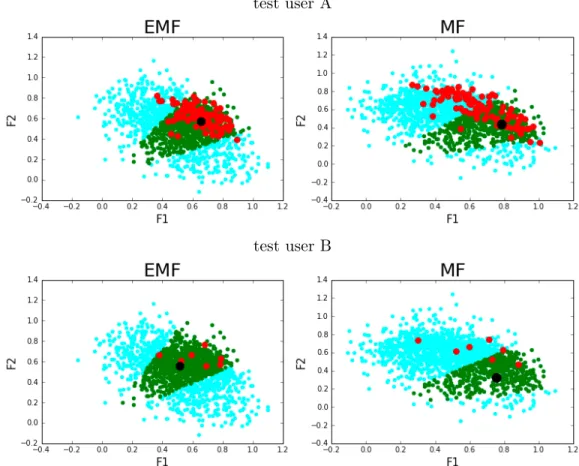
3.7 Red points = explainable items, green points = relevant items, Cyan points = remaining items, black point = sample user. For two sample users (top and bottom rows), the items are represented in the latent space (f = 2, for visualization purpose). In each case, EMF has resulted in explainable items to be located closer to the user and in the green area (relevant items for recommendations). . . 48
3.8 Conditional RBM for explainable recommendations. . . 50
4.2 Corresponding Top-3 NSE-based explanations generated for the recommen-dations shown in Table 4.2. Recommenrecommen-dations/explanations are generated using asymmetric MF for Sample User A. . . 55 4.3 Corresponding Top-3 ISE-based explanations generated for the
recommen-dations shown in Table 4.2. Recommenrecommen-dations/explanations are generated using asymmetric MF for Sample User A. . . 56 4.4 Genre frequency of the rated movies by Active User B. . . 57 4.5 Corresponding Top-3 NSE-based explanations generated for the
recommen-dations shown in Table 4.4. Recommenrecommen-dations/explanations are generated using asymmetric MF for Sample User B. . . 58 4.6 Corresponding Top-3 ISE-based explanations generated for the
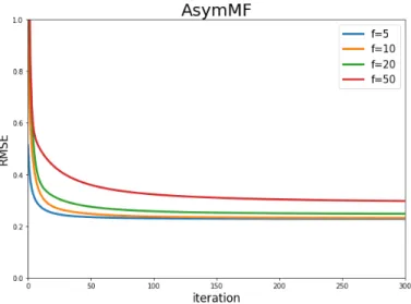
recommen-dations shown in Table 4.4. Recommenrecommen-dations/explanations are generated using asymmetric MF for Sample User B. . . 59 4.7 RMSE calculated over the testing data with each iteration decreases. The
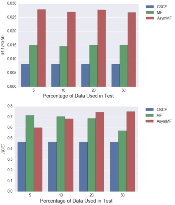
setting for this experiment isα= 0.001 and β = 0.01, when varyingf. . . . 60 4.8 Comparison of accuracy when varying the percentage of data used in the test. 61 4.9 Objective function, J, calculated over the training data in each iteration
decreases until convergence. The setting for this experiment is f = 5,|N.|=
50, andθ= 0 for all three explanation styles. . . 62 4.10 Comparison of accuracy when varyingf. . . 63 4.11 Comparison of accuracy when varying|N.|. . . 64
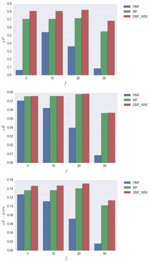
4.12 Comparison of user basedxP,xR, andxF scorewhen varyingf. ForEM F techniques we set |N.|= 50. . . 65
4.13 Comparison of item based xP,xR, and xF scorewhen varying f. ForEM F techniques we set |N.|= 50. . . 66
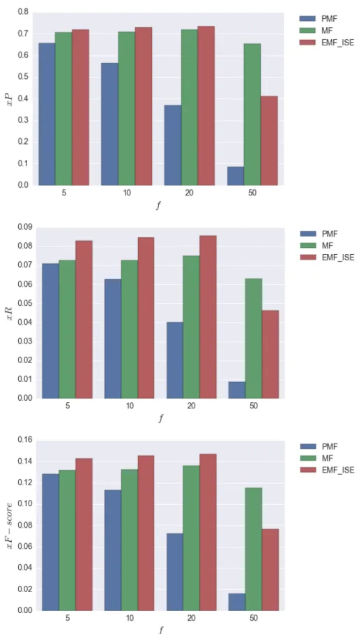
4.14 Comparison of feature based xP, xR, and xF score when varying f. For EM F techniques we set |N.|= 50. . . 67 4.15 Comparison of user basedxP,xR, and xF score when varying|N.|. . . 68
4.16 Comparison of item basedxP,xR, and xF scorewhen varying|N.|. . . 69
4.17 Comparison of accuracy when varyingf. ForEM Ftechniques we set|N(u)|= 50. . . 73 4.18 Comparison of accuracy when varying|N.|. . . 74
4.19 Comparison of user basedxP,xR, and xF scorewhen varying f. ForERBM techniques we set |N.|= 50. . . 75
4.20 Comparison of item basedxP,xR, andxF scorewhen varyingf. ForERBM techniques we set |N.|= 50. . . 76
4.21 Comparison of feature based xP, xR, and xF score when varying f. For ERBM techniques we set|N.|= 50. . . 77 4.22 Comparison of user basedxP,xR, and xF score when varying|N.|. . . 78
4.23 Comparison of item basedxP,xR, and xF scorewhen varying|N.|. . . 79
4.24 Example of an automated explanation generated for the recommended movie: “Lost Highway (1997)” using the EM FN SE technique. . . 80
4.25 Example of the automated explanation generated for the recommended movie: “McHale’s Navy (1997)” using theEM FISE technique. . . 81
4.26 Example of the automated explanation generated for the recommended movie: “That Darn Cat! (1965)” using theEM FKSE technique. . . 81
4.27 Comparison between two explanations for a test user where the explainability of the itemi1 on the left is higher than item i2 one on the right. . . 82 4.28 Example of movies shown to the user to rate. . . 84 4.29 Example of a recommendation with explanation presented to the user. . . . 85 4.30 Horizontal bar graph of the answers to the questions in Table 4.8. . . 87 4.31 Horizontal bar graph of the answers of people in the group ”low” to the
questions in Table 4.8. . . 88 4.32 Horizontal bar graph of the answers of people in the group ”medium” to the
4.33 Horizontal bar graph of the answers of people in the group ”high” to the
questions in Table 4.8. . . 88
4.34 Heat-map plot of the answers to the questions in Table 4.8. . . 89
4.35 Heat-map plot of the answers of people in the group ”low” to the questions in Table 4.8. . . 89
4.36 Heat-map plot of the answers of people in the group ”medium” to the ques-tions in Table 4.8. . . 90
4.37 Heat-map plot of the answers of people in the group ”high” to the questions in Table 4.8. . . 90
4.38 Distribution of the participants’ gender. . . 91
4.39 Distribution of the participants’ age. . . 91
4.40 Distribution of the participants’ weekly hours watching movies. . . 91
4.41 Distribution of the participants’ familiarity with recommender systems. . . 92
4.42 Distribution of the participants’ favorite genres. . . 92
4.43 Visualization of group pairs’ differences for “transparency”. . . 95
LIST OF ALGORITHMS
ALGORITHM Page
2.1 Basic Alternating Least Square (ALS) Algorithm . . . 17
2.2 Basic SGD Algorithm for MF . . . 18
3.1 NSE-Based Explanation Generation Algorithm in the Latent Space . . . 37
3.2 ISE-Based Explanation Generation Algorithm in the Latent Space . . . 38
CHAPTER 1
INTRODUCTION
Machine learning (ML) models are being used increasingly in many sectors, ranging from health and education to e-commerce and criminal investigation. Hence, these Artificial Intelligence (AI) systems are starting to affect the lives of more and more human beings. Examples include risk modeling and decision making in insurance, education (admission and success prediction), credit scoring, medical, criminal investigation and predicting re-cidivism, etc. Without the intelligent systems’ ability toexplain their decisions and actions
to the human users, the effectiveness of these systems can be limited. Users may require
understandingandtrusting predictions made by these systems before making decisions with
an inherent risk, as a result of these predictions [1].
Furthermore, AI models are susceptible to bias that stems from the data itself or from systemic social biases that generated the data (e.g. recidivism, arrests). As such, models that are learned from real world data can become unethical if their outputs discriminate, albeit unintentionally, against a certain group of people. While building ethical and fair models seems like the ultimate and ideal goal, the minimum and urgent criterion that ML models should satisfy istransparency, and this could be the first step in the direction toward
fair and ethical models. Therefore, designing explainable intelligent systems that facilitate conveying the reasoning behind the results is of great importance.
Recommender systems are a special kind of ML AI systems that suggest interesting items to users in various decision making situations, with suggested items ranging from songs and books to courses and news. Recommender systems represent a valuable means of helping online users with information overload and they have recently become powerful pillars in e-commerce and information retrieval (IR). Collaborative filtering (CF) recommendation
systems try to suggest items of interest (e.g., movies, songs, books, applications, websites and travel destinations) to a user based on their user profile which can be explicit (e.g. user ratings) or implicit (e.g. their browsing or purchase history) [2,3]. CF recommender systems provide recommendations to users based on the similarity between users or between items, giving rise to neighborhood-based CF approaches, which can be user-based or item-based. Other sources of information such as users’ demographic data and items’ features may be used to provide a user with a list of items that maximize the user’s utility or satisfaction. These recommender systems exploit rating or purchase history as their main source of input information. When there is not enough history available for new users or new items in the system, a CF system cannot provide good recommendations. This is known as the cold-start problem, and can be considered as an extreme case of sparse input data.
It is important for a recommender system to provide explanations for recommenda-tions. In fact, most commercial recommender systems provide simple explanations to the users, and this can enhance the user’s trust and acceptance. Even long before automated recommender systems, a medical expert, system’s explanation of the reasoning behind a suggestion, has been found to be critical to the users’ acceptance of the system’s sugges-tion [4]. Amazon’s recommender system shows similar items that the user (or other similar users) have bought or viewed, when recommending a new item. The Netflix recommender system justifies its movie suggestions by listing similar movies obtained from the user’s so-cial network. When an interpretable model is used in a recommender system, it has been shown that explanations can help users make more accurate decisions; hence, improving user satisfaction and acceptance of recommendations [5–7].
In Figure 1.1, four different explanation examples are shown, where (1) and (3), are based on the ratings of the active user’s most similar users (neighbors) that is called Neighbor Style Explanation (NSE); (3) is a feature-based explanation that is based on the content and keyword features, and is called Keyword Style Explanation (KSE); while (4) is based on the active users ratings of items that are similar to the recommended item, and is called Item Style Explanation (ISE) [6].
(1) (2)
(3) (4)
Figure 1.1: Four different explanation style examples.
Machine Learning techniques used for recommender systems can be categorized in two families: White-Box methods (WB), such as Decision Trees [8, 9], and production rule learners [10, 11], which are interpretable and essentially come with explanations. On the other hand, Black-Box (BB) methods such as Artificial Neural Networks [12], Support Vec-tor Machines [13], Ensemble Methods [14], and Matrix FacVec-torization (MF) [15, 16] produce opaque models which are not easily interpretable by humans. Most accurate recommender systems, available nowadays, developed mainly in research labs and in some cases for com-mercial use, are BB models. The most popular BB models, for recommender systems, nowadays are based on Matrix Factorization models, with deep learning networks, also recently becoming another popular BB model. MF methods are accurate CF approaches that map users and items to low-dimensional feature vectors [17]. MF methods fit a model to the known ratings and use the model for further predictions. In most MF-based tech-niques, predictions are not interpretable and cannot be justified to the user as easily as in neighborhood-based CF methods. Although a few of these provide some form of explana-tion, it is not clear why the system is recommending a specific item, which may result in users not trusting the suggestions of the recommender system. One way to communicate
explanations would be based on identifying similar users and/or items in the latent space and presenting the most similar users and/or items as the explanation. The drawback of this method is that the way the explanation is generated does not necessarily comply with the learned ML model. This is because the solution to the MF optimization problem does not guarantee that the most similar users to an active user, who have liked the system’s suggestion, are necessarily the active user’s neighbors in the latent space. Thus, the only way to assess the quality of the recommendation for the user is to try the item. This, however, is contrary to one of the goals of a recommendation system, which is reducing the time that users spend on exploring items.
It would be very desirable and beneficial to design recommender systems that can give accurate suggestions, which, at the same time, facilitate conveying the reasoning behind the recommendations to the user. However, a main challenge in designing a recommender system is whether to choose an explainable technique with moderate prediction accuracy or a more accurate technique (such as MF) which does not give explainable recommendations.
1.1 Problem Statement
Due to the trade-off between a machine learning model’s prediction accuracy and its interpretability [18], it is generally very challenging to achieve both accuracy and explain-ability. Therefore, it is common, in many applications, to opt for accuracy at the expense of interpretability.
Our research question is: can we design a model-based recommender engine that suggests items that are explainable, while recommendations remain accurate? In order to
answer this question, we define explainability and hypothesize that recommendations that have higher explainability value, help users make better decisions, therefore they are more effective.
1.1.1 Assumptions
We assume that the BB recommender system is mainly rooted in a latent factor-based or deep learning model using ratings as the primary input and possibly augmented with item or user attributes into a hybrid CF system. We also assume that the input to the recommendations and the input to the explanations are not constrained to be exactly the same. This is because an input can contribute to empowering a BB model’s training, while not necessarily being a good source of human explanation. Most studies in the literature study the effect of explanations as a separate module from the recommender module [5,6,19]. The focus of their studies are mostly on the types and formats or visualizations of the explanations regardless of the recommender module [19, 20].
Our current scope is limited to CF recommendations where explanations for recom-mended items are in one of the three main explanation styles: NSE, ISE or KSE, as shown in Figure 1.1. We encode the user-item explainability relationship in a graph. While other methods in the literature have used graph structures to find a better representation of data points in lower spaces, we further incorporate the explainability graph in the design of the MF model to be able to generateexplainable recommendations.
1.2 Research Contributions
1. We present a cross-modal recommender engine that leverages multiple domains of data to retrieve similar items and recommend the most relevant items to the user. We show how this approach can automatically generate explanations for the recommendations and also has the potential to alleviate the cold-start problem, one of the most notorious limitations of Collaborative Filtering (CF) techniques.
2. We propose a probabilistic formulation for measuring the explainability of Neighbor-Style Explanation (NSE), Influence Neighbor-Style Explanation (ISE), and feature Neighbor-Style Expla-nation (KSE) for recommendations.
explain-able recommendations that can leverage the accurate predictions of MF and the trans-parency of neighborhood-based CF algorithms. In our method, explainability can be directly formulated based on the rating distribution within the user’s or item’s neigh-borhood. If many neighbors have rated the recommended item, or the user have rated many similar items to the recommended item, then this provides a basis upon which to explain the recommendations.
4. We propose an explainability metric based on Keyword Style Explanation that uses item content features to generate explanations and recommend explainable items. 5. We encode the user-item explainability relationship in a graph. While other methods
in the literature have used graph structures to find a better representation of data points in lower spaces, we further incorporate the explainability graph in the design of the MF model to be able to generate explainable recommendations.
6. We propose an explanation-aware neural network using constrained Restricted Boltz-mann Machines (RBM) for CF to recommend items that are explainable.
7. We propose offline metrics to evaluate the explainability of recommender systems. 8. We present user study experiments for online evaluation of our proposed explainable
CHAPTER 2
BACKGROUND AND LITERATURE REVIEW
“We are leaving the Information Age and entering the Recommendation Age [21].” In the past, gathering information to make effective and efficient decisions was difficult, and recommendations from others and their experience were a guide to us through this lack of knowledge. Today, we are overloaded with information which means we have more choices and therefore making choices is becoming even harder. Recommender systems can act as shortcuts through the information to help us narrow our choices, and obtain relevant information.
Recommender systems are used in many websites to personalize the experience of a user based on their past history, item content, or user demographic information. Among recommender systems, collaborative filtering (CF) is an effective recommendation approach in which the preference of a user can be predicted based on information from other users that share similar interests, without requiring any content information about the recommended items. This chapter presents a thorough overview of the methods in the literature. In Section 2.1, we review recommender system approaches, and their challenges such as the cold-start problem and the importance of providing explanations. Section 2.2 is devoted to latent factor models including Matrix Factorization and Restricted Boltzmann Machines. Section 2.4 presents the review of recommendation explanation mechanisms. Finally, in Section 2.5, we summarize the chapter.
2.1 Recommendation Systems
The recommender problem may be defined as approximating a utility function that predicts how a user will like an item automatically. Utility is usually represented by user
ratings, however it could be any function. The recommendation process is based on the past behavior of the users, the relations between the users or the items, item similarity based on the content, and finally context [22].
Formal definition of a recommender system: let U be the set of users, I be the set of possible recommendable items, andf be the utility function measuring the usefulness of itemi to user u. For each user u belonging to U, we want to choose items belonging toI, that maximize f, i.e.,
∀u U, i∗=argmax(f(u, i)) s.t. i I (2.1)
Recommender systems can be divided based on which data and which mechanism they use to make recommendations. The main categories of recommender systems are
content-based filtering (CBF), collaborative filtering (CF), and hybrid methods. Content-based filtering makes recommendations Content-based on the content of the items (e.g. text or images) and the content of the user profiles. The similarity between an object of interest and the items that the user has bought, viewed, or ranked before, is calculated based on a user or item profile, and is used as the basis for the recommendation. Content-based approaches require ratings made by only the user herself in contrast to collaborative filtering models that also use the ratings of other users who are similar to the target user in order to derive the recommendations. Collaborative filtering algorithms exploit the historical ratings and preferences of the active user’s preference and the like-minded users to suggest items or to predict the utility of an item for a particular user. Content-based characteristics can be combined with collaborative filtering models to improve the results of recommendation. This type of recommendation is known as a hybrid recommendation [23].
In a typical CF framework, there are m users: U = {u1, u2, ..., um} and n items:
I ={i1, i2, ..., in}. The set of items that the userui has expressed her opinions about isIui. Note that it is possible for Iui to be a null set. The opinions can be explicitly provided by the user as a rating score, or can be implicitly derived from the purchase logs or web history of the user [24,25]. In 2.1, an example of a utility matrix is shown that represents the users’
Figure 2.1: A user-book ratings matrix, representing ratings of books on a scale of 1-5.
ratings of books on a scale of 1-5, with 5 being the highest rating. Users are shown in the rows and books are shown in the columns. The number of stars in each cell represents the rating of the user in the corresponding row on the specific book in the corresponding column, while blank cells show the situation where no rating is available. CF methods estimate the appropriate value for some of the blank cells (cells filled in with a question mark).
For the active user ua, the result of the CF algorithm can take two forms (that do
not necessarily have direct relationship [26]):
1. A numerical value, which is a predicted value for the likeness of item i /∈Iua for the active userua.
2. A list of top-N recommended items for the active user ua. The set of top-N
recom-mended items and the items that the user has already purchased or rated must not have any overlap.1
2.2 shows the general framework for the collaborative filtering process on the rating data that is shown in 2.1.
CF techniques can be classified into two groups: memory-based methods and
model-based methods [27].
1The exception rule is ignored in some cases, such as certain eBay and e-learning transactions, as well as
Figure 2.2: Collaborative filtering process.
2.1.1 Memory-based Methods
Memory-based methods provide recommendations based on the user or similar-item neighborhood around the target user or the target similar-item. Depending on whether the obtained neighbors are similar users or items, memory based methods are classified as user-based algorithms or item-based algorithms. Similar to the idea of nearest neighbor classification, after computing the similarities, the neighbors are aggregated to get the top-N most similar users or items [28–30]. The similarity w between users a and u can be computed usingPearson’s correlation coefficient [31]:
w(a, u) = Pm j=1(ra,j −r¯a)(ru,j−r¯u) q Pm j=1(ra,j −r¯a)2 Pm j=1(ru,j−r¯u)2 (2.2)
wheremis the total number of items that bothaanduhave rated. ra,j is the rating
that user a gave for item j and ru,j is the rating of user u on item j. ¯ra and ¯ru are the
averages of user a’s ratings and user u’s ratings for all items, respectively. Similarly, the similarity between items kand ican be computed using the following formula:
w(k, i) = Pm j=1(rj,k−r¯k)(rj,i−r¯i) q Pm j=1(rj,k−r¯k)2Pmj=1(rj,i−r¯i)2 (2.3)
wheremis the total number of users that rated both itemskandi. rj,k is the rating
that userjgave to itemkandrj,iis the rating of userjto itemi. ¯rkand ¯ri are the average
ratings of itemsk andi, respectively.
similarity between two users or two items. The similarity between two users a and u is defined as: Cos(a, u) = m X j=1 ra,j q Pm j=1ra,j2 ru,j q Pm j=1ru,j2 (2.4)
wheremis the total number of items that bothaanduhave rated. ra,j is the rating
that useragave for itemjandru,jis the rating of useruon itemj. Similarly, the similarity
between items kand i, can be computed using the following formula:
Cos(k, i) = m X j=1 r,j,k q Pm j=1r2j,k rj,i q Pm j=1rj,i2 (2.5)
wheremis the total number of users that rated both itemskandi. rj,k is the rating
that userj gave to itemk and rj,i is the rating of userj on itemi.
Recommender Systems traditionally use the Pearson’s correlation or cosine similar-ity, however, many other similarity measures can be used. Ellen Spertus et al. [32] evaluated six different similarity measures in the context of the Orkut social network. The best re-sults were for recommendations generated using the cosine similarity. On the other hand, Lathia et al. [33] studied several similarity measures in the context of recommender systems and concluded that the prediction accuracy was not affected by the choice of the similarity measure.
One drawback of memory-based methods is that computing accurate similarities Another drawback is that the search for neighbors among a large user population of potential neighbors forms a bottleneck in the user-based neighborhood CF methods [28]. Item-based techniques may be able to avoid this bottleneck because item neighborhoods are relatively static compared to user neighborhoods.
2.1.2 Model-based Methods
Model-based CF methods use the rating data to train a system to make predictions based on a learned model. The model can be built using different machine learning
al-gorithms such as Bayesian networks [34, 35], clustering [36], matrix factorization [15], and rule-based approaches [37].
Some representative methods include [3, 38–40]. Among the model-based CF meth-ods, matrix factorization based methods [27] have been the most popular in recent years, and they have proven to address collaborative filtering challenges such as scalability and sparsity effectively [16, 41, 42]. Memory-based and model-based CF approaches can be combined to form hybrid CF approaches to improve the recommendations [43, 44]. More recent work uses textual reviews and opinions to improve the performance of rating prediction [45–47]. Even though CF tasks have achieved some success in providing recommendations to the users, there are additional challenges that they still need to address to produce high quality predictions, such as data sparsity and the cold-start problem (new items or new users) [48]. Usually, in recommender systems, there is a large set of items to evaluate. This results in an extremely sparse user-item matrix for collaborative filtering [27]. The cold-start problem happens when a new user or a new item enters the system. The system cannot recommend items to the new user until some of their rating information becomes available; similarly, new items cannot be recommended until some users have rated them [43, 48].
2.1.3 The Sparsity Problem
Recommender systems generally have to deal with data in a very high dimensional space. This space is usually very sparse and only a limited number of features are available for each object. For example, in Amazon.com, only a few ratings out of billions of items are typically available from each user. In a high dimensional space, all objects tend to be dissimilar and finding objects that form groups with similar properties becomes critical. This is because there is no intuitive notion of density or distance between points as in low dimensional spaces. This is known as the Curse of Dimensionality [22].
To overcome this problem, dimensionality reduction techniques are typically used to convert the high dimensional space to a new lower-dimensional space. The most relevant methods for dimensionality reduction in recommender systems are Matrix Factorization
(MF) methods. These techniques will be presented in section 2.2.
2.1.4 The Cold start problem
The cold-start problem is a notorious problem for CF systems. It happens when rec-ommendations have to be made for new users in the system, or when new items that no one has rated yet need to be recommended. Providing an accurate and efficient recommendation result in the cold start case is a key challenge in CF [49]. Cold start problems can occur in three cases: (a) recommendation on existing items for new users, (b) recommendation for existing users on new items, and (c) recommendations on new items for new users.
When new users enter the system, they are asked to provide their ratings for different items to acquire information for CF. Usually in CBF, the system asks new users a series of questions to generate her initial profile with her explicitly stated preferences. As a user likes or consumes more items, the system can update her profile and give more weights to the content features of the items that she consumed. In these approaches, the recommended items are similar to the items that were previously consumed by the user. This can result in lack of diversity and therefore low satisfaction with recommendation results.
One possible remedy for the cold-start problem is to exploit user and item attributes because they can help create a bridge between existing users or items and new users or items. Rashid et al. [50] propose several strategies that can be incorporated in CF algorithms to learn about the new users in the system. These techniques, which present items to new users, range from random item selection to methods that exploit database queries such as choosing popular items. Park and Chu [51] proposed a predictive regression model that incorporates demographic information as well as content features to tackle the cold-start problem. Shaw et al. [52] used association rule mining to expand user profiles and provide more accurate recommendations for new users. However, extracting rules from large datasets with a very large number of multi-valued attributes is often computationally prohibitive. Golbandi et al. [53] presented a model for profiling new users in the system by eliciting the opinion of users about items. The core of their method is an efficient decision-tree-based recommender
algorithm, suitable for an adaptive bootstrap process. In [54], a functional matrix factor-ization (fMF) was proposed. An initial interview is performed to acquire information from the new user. To construct the adaptive interview, a decision tree is learned with each node being an interview question. Zhang and Li [55] proposed a solution for the cold start that makes use of social tags. Their recommendation algorithm considers social tags as a bridge that connects users and items. Shein et al. [56] proposed a probabilistic model for combining collaborative filtering and content information to recommend new items to the users. They used the EM algorithm to fit the model to the data.
2.2 Latent Factor Models
As described in Section 2.1.3, one drawback of memory-based CF methods is that it is solely based on the co-rated items and does not consider the hidden interests and topics that similar users and items share. Latent factor models, that are also known as Matrix Factorization (MF) models, are model-based techniques that leverage the idea that ratings are influenced by a set of lower rankfactors, such as movie genres, characters, etc. In these
type of models, both users and items are projected into a new latent feature space using an objective function. Similar to MF techniques, Restricted Boltzmann Machines (RBM) also perform latent factor discovery and can be categorized into latent factor models. These latent factors are solved using optimization techniques. In this section, an overview of some of the most common latent factor models in the literature is given.
2.2.1 Principal Component Analysis (PCA)
PCA is a statistical method that converts a set of data points observed from possibly correlated variables into a set of points with linearly uncorrelated variables that are called principal components. The amount of variance captured by the first component is larger than the second component and so on. PCA is applicable when the data set is mostly Gaussian.
2.2.2 Singular Value Decomposition (SVD)
SVD is another powerful method for dimensionality reduction in Recommender Sys-tems, which allows for extracting concepts from the high dimensional data in a new space. Given the matrix X(n×m), X can be decomposed intoX =UΣWT, where Σ is a k-by-k rectangular diagonal matrix of positive numbers, called the singular values of X; U is an n-by-k matrix, the columns of which are orthogonal unit vectors of length ncalled the left singular vectors ofX; andW is a m-by-k matrix whose columns are orthogonal unit vectors of lengthm and called the right singular vectors ofX. The k Eigenvalues in Σ are ordered in decreasing magnitude. To approximate X, the Eigenvalues matrix Σ can be truncated up to row i, resulting in Xi: Xi = UiΣiWiT which is the closest rank-i matrix to X. In
terms of factorization computation,W is equivalent to the eigenvectors ofXTX, sinceXTX can be written as: XTX = WΣUTUΣWT = WΣ2WT. Similarly, U is equivalent to the eigenvectors ofXXT.
Although Matrix Factorization methods such as PCA and SVD can be used in preprocessing to lower the dimensionality, in recent years they have been employed as independent approaches to Recommender Systems.
2.2.3 Matrix Factorization (MF)
MF is a family of latent factor algorithms where a data matrix,X, is factorized into two lower rank approximated matrices P and Qas follows:
Xn×m 'Pn×fQTm×f (2.6)
f is the rank of matrices P and Q, and it is selected such that f min(m, n), so that the number of elements in the decomposition matrices is far less than the number of elements of the original matrix: nf +f mnm.
One of the common applications of matrix factorization is in collaborative filtering recommender systems [15]. The Netflix prize competition has contributed a lot to the popularity of matrix factorization in recommender systems [15]. In this context, MF takes
Figure 2.3: Decomposed matrices with rank 2.
as input the user-item rating data and decomposes users and movies into a set of latent factors that define a new latent space, which can be thought of as concepts or categories. 2.3 shows an example of user and item decomposition matrices with f = 2, where MF projected onto a lower dimensional latent space extracted using matrix factorization. An effectively intuitive interpretability of the resulting factors, as shown in 2.3 in this fictitious example, can make MF especially interesting for many applications.
MF algorithms learn the factors pu ∈ Rf and qi ∈ Rf, which are the lower-rank
representations of useruand item iin a latent space of reduced dimensionalityf. In order to estimate pu and qi, the following objective function is minimized [17]:
JM F = X (u,i)∈R (ru,i−puqTi )2+ β 2(||pu|| 2+||q i||2) (2.7)
where R is the set of available ratings for the (u, i) pairs. The regularization term (||pu||2+||qi||2) with the regularization coefficient,β, control the smoothness and sparseness
of the resulting factors. This optimization problem is not convex; however, it is convex with respect to matrixP only or matrixQonly. It can therefore be solved by using arithmetic or
multiplicative updates forP andQ. In Sections 2.2.3.1 and 2.2.3.2, two of the most common algorithms in the literature, for solving MF, are reviewed.
2.2.3.1 Alternating Least Squares
Alternating Least Square (ALS) is an iterative approach, which fixesP orQin each iteration. Although 2.7 is not convex, it is convex in either P or Q. However, it does not guarantee that the matrices found are the global solutions and provides only a local minimum to the MF problem. The ALS method is outlined in Algorithm 2.1 [16, 57]. Algorithm 2.1 Basic Alternating Least Square (ALS) Algorithm
Input: data matrixR, number of factors f Output: optimal matrices Pand Q
1. Initialize matrix P(for example randomly) 2. Repeat
3. Solve for Qusing: PTPQ=PTR 4. Solve for Pusing: QQTPT =QRT 5. Until the cost function converges
2.2.3.2 Stochastic Gradient Descent
In the basic Stochastic Gradient Descent (SGD) approach,pu andqiare modified in
each iteration by an amount proportional to the value of the gradient [58]. The derivative of JM F with respect to pu and qi is:
∂JM F ∂pu =−2(ru,i−puqiT)qi+βpu (2.8) ∂JM F ∂qi =−2(ru.i−puqTi )pi+βqi (2.9)
Given Formula 2.8 and 2.9 the SGD update rules are as follows:
qi+1 ←qi+α(2(ru,i−puqiT)pu−βqi) (2.11)
where α and β are the learning rates. Algorithm 2.2 shows the application of SGD update rules iteratively until convergence.
Algorithm 2.2 Basic SGD Algorithm for MF
Input: data matrix R, number of factorsf, learning rates α and β Output: optimal matricesPand Q
1. Initialize matrix P and Q(for example randomly) 2. Repeat
3. For every (u,i) pair
4. updatepu : pnewu ←pu+α(2(ru,i−puqiT)qi−βpu)
5. updateqi : qinew←qi+α(2(ru,i−puqTi )pu−βqi)
6. End for
7. Until the cost function converges
Choosing the right values for α and β is very important in the gradient decent algorithms. If these values are too small, the updates will converge too soon, and if large values are selected, it will not converge.
2.2.4 Restricted Boltzmann Machines (RBM)
Restricted Boltzmann Machines (RBM) is another kind of latent factor model that extracts a smaller set of hidden variables from the input data, that can be used as data representation. RBM is a two layer stochastic neural network consisting of visible and hidden units that are connected bidirectionally. Each visible unit is connected to all the hidden units in an undirected form. No visible/hidden unit is connected to any other visible/hidden unit. The stochastic, binary visible units encode user preferences on the items from the training data, therefore the state of every visible unit is known. Hidden units are also stochastic, binary variables that capture the latent features. A probability
p(v, h) is assigned to each combination hidden unit, h, and visible unit,v:
p(v, h) = e −E(v,h)
Z (2.12)
where E is the energy of the system and Z is a normalizing factor [59]. E can be defined as follows: E(v, h) =− n X i=1 m X j=1 wijhivj− m X j=1 bjvj − n X i=1 cihi (2.13)
wheremand nare the numbers of visible units and hidden units, respectively,wij is a real
valued weight associated with the edge between the units of visible units and hidden units, and bj and ci are real valued bias terms associated with the visible units and hidden units
respectively. The network graph representation of an RBM is shown in Figure 2.4. The conditional probabilitiesp(hj = 1|v) and p(vi = 1|h) are defined as:
p(hi= 1|v) =σ(ci+ m X j=1 vjwij) (2.14) p(vj = 1|h) =σ(bj+ n X i=1 hiwij) (2.15)
whereσ(x) is the logistic function (1+1e−x). To train for the weights, a Contrastive Divergence method was proposed by Hinton [59].
Salakhutdinov et al. [60], proposed an RBM framework for CF. Their model assumes one RBM for each user and takes only rated items into consideration when learning the weights. They presented the results of their approach on the Netflix data and showed that their technique was more accurate than Netflix’s own system. The focus of this RBM approach was on evaluating the performance of the proposed system in terms of rating prediction.
2.3 Comprehensible Classification Models
In this section, we review interpretable classification models because explanations are related to interpretability of predictive models.
Figure 2.4: An RBM network with nhidden and mvisible units.
In the context of machine learning, interpretability means “explaining or presenting in understandable terms” [61]. In addition, interpretability and explanations can help to determine if qualities such as fairness, privacy, causality, usability and trust are met [62].
Doshi-Velez and Kim [62] presented a taxonomy of approaches for the evaluation of interpretability in ML models in general: application-grounded, human-grounded, and functionality-grounded. Application-grounded and human grounded evaluation approaches are both user-based, while the functionality-grounded approach does not require human evaluation and uses some definition of the interpretability for the evaluation. Experiments can be designed based on different factors, such as global vs local, which considers the general patterns existing in the model as global, while considering local reasoning behind the specific prediction of the model as local [62]. The former is usually helpful for the designer and developer of the model when understanding or detecting bias or causality in the model. The latter can be aimed at the end user of the systems to understand the justifications of the system decisions.
Ribeiro et al. [63] proposed an explanation technique that explains the prediction of the classifiers locally, using a learned model. Their proposed explanation conveys the relationship between the features (such as words in texts or parts in images) and the pre-dictions; and helps in feature engineering to improve the generalization of the classifier. This can help in evaluating the model to be trusted in real world situations, in addition to using the offline accuracy evaluation metrics.
mod-els (decision trees, decision tables, classification rules, nearest neighbors, and Bayesian network classifiers). It is important to distinguish understanding or interpreting an entire model (which the paper does) from explaining a single prediction (which is the focus of this dissertation). In addition, we note that Freitas overviews the problem from several perspectives and discusses the motivations for comprehensible classifier models, which are: 1. Trusting the model: Regardless of accuracy, users are more prone to trusting a model
if they can comprehend why it made the predictions that it did.
2. Legal requirements, in some cases like risk modeling, require a justification in case of denying credit to an applicant.
3. In certain scientific domains such as bioinformatics, new insights can be gained from understanding the model, and can lead to new hypothesis formation and discoveries. 4. In some cases, a better understanding can help detect learned patterns in the classifi-cation model that are not really stable and inherent in the domain, but rather result from overfitting to the training data, thus they help detect the data shift problem: i.e., when the new instances deviate in their distribution from past training data; we note that concept drift (i.e. when a previously learned and accurate model no longer fits the new data because of changes in patterns of the data) can be considered as a special case of the data shift.
Understanding the logic behind the model and predictions (in other words, comprehension)
can reveal to the user the fact that the (new) data has outpaced the model. The user can then realize that the model has gotten old and needs to be updated with a new round of learning on new data. Various interpretation methods exist depending on the family of clas-sifier models: decision trees, rule sets, decision tables, nearest neighbors. Different studies have shown that the interpretability of entire classifier models depends on the application domain and the data, with findings that sometimes contradict each other. Regardless of all the findings in interpreting models, we note that the task of interpreting an “entire classifier
model” (e.g. a complete decision tree or a set of 500 rules) is different from that of one user trying to understand the rationale behind a “single prediction/recommendation” instance. That said, we find Freitas’ review to be very important for this work: first he argues that model size alone is not sufficient to measure model interpretability, as some models’ complexity is beyond mere size and small models can actually hurt the user’s trust in the system (a notorious example is decision stump models (1-level trees) in the medical or legal domain which do not offer enough evidence to be able to judge a prediction model and would actually lead to the same explanation for each new test instance. Also, extremely small models would likely suffer in accuracy. Second, the work on interpreting rule-based models and nearest neighbor models can be useful to us because it is closest to the CF mechanisms we study. For nearest neighbor models, Freitas [64] mentions that attribute values of nearest neighbors can help provide explanations for predictions, and that showing these values in decreasing order of relevance (based on an attribute weighting mechanism) is a sensible strategy. Another strategy is to show the nearest prototypes of training instances, for example after clustering the training instances. However, in both of these strategies, Freitas [64] was motivating types of entire models rather than individual prediction explanations in the context of recommending thousands of items.
2.4 Explanation Mechanisms in Collaborative Filtering
Most recommendations are the result of black box systems which do not provide the reasoning behind their suggestions to the user. While the user might trust a recommenda-tion to listen to a song, s/he is less willing to act based on recommendarecommenda-tions in higher risk content domains such as renting a holiday resort. Herlocker et al. presented evidence that showed explanations improves the acceptance of recommender systems by the user [65]. The explanation may, or may not reflect the underlying algorithm used by the system. Explanations can be given using words related to item features or user demographic data, but these cannot be done easily in CF approaches. They vary between simple explanation formats such as: “people also viewed” in e-commerce websites [66] to the more recent
so-cial relationships and soso-cial tag based explanations [67, 68]. Bilgic & Mooney [69] showed how explaining recommendations can improve the user’s estimation of the item’s quality and help users make more accurate decisions (i.e. user satisfaction). In black box models, the technology behind generating recommendations may not be conveyable to the user. However, one way to provide explanations to justify any recommender system’s output is by providing the system’s past performance. Explanations help provide transparency into these type of systems.
2.4.1 Benefits of Explanation
Explanations can help the user detect errors in recommender systems. The output of recommender systems is prone to error which can be due to data errors or the model not matching the user’s requirements. Data errors are intrinsic characteristics of collaborative filtering systems which can happen because of missing and sparse data, poor or bad data, and high variance data.
In addition to trust and error detection benefits, explanations can add justifica-tion and acceptance. Justificajustifica-tion gives the user an understanding of the reasoning in the recommendation process which helps the user decide how much confidence to put in the output. Acceptance of a recommender system can be improved after an explanation since the system’s limits and strengths become more visible to the users.
Tintarev and Masthoff [70] studied additional aims of explanations such as trust, effectiveness, and satisfaction. A good explanation would increase the perceived quality of the recommendation and adoption of the recommender system by the user.
We can summarize the benefits of explanation in the following list:
• Perceived quality and satisfaction: According to Pu et al., the key factor in a successful
recommendation system is its quality, which will affect the acceptance of the system by the user and interaction with the recommender system [71]. Explanation is another factor in increasing the perceived quality. Descriptions and explanations have been found to be correlated with the perceived usefulness of the recommender system,
thereby increasing the overall satisfaction of the user [72].
• Trust: Studies by [65, 70, 73] have shown that a good explanation interface could
increase users’ trust and satisfaction by providing information to justify the recom-mendations. This in turn increases user involvement and educates users on the internal logic of the system. Trust in the recommender system also depends on the accuracy of the recommendation. Good explanations may not compensate for poor recommen-dations, however if a user understands why a bad recommendation has been made, they may be more confident in the system.
• Transparency and scrutability: Explanations can provide the user with the logic
be-hind the recommendation to clarify how a recommendation was chosen. The impor-tance of transparency also known as “visibility of system status” has been confirmed by user studies of recommender systems [72]. Following transparency, recommender systems should allow the user to correct the reasoning and assumptions made where needed.
• Persuasiveness: The recommender system could persuade the user into buying or
trying a recommended item, whether the prediction is accurate or not.
• Effectiveness: Effectiveness is highly dependent on the accuracy of the
recommenda-tion. An effective explanation can assist the user to make better decisions according to their preference, by giving the user a broad range of options, including a new domain, or new range of products.
2.4.2 Explanation Approaches and Algorithms
Most recommender systems in the literature are black boxes. Although, a few of them provide some form of explanation, it is still not clear to the user why a specific item is being suggested. This results in users not trusting the suggestions of the recommender system. However, the way that white box models perform are close to the conceptual model of the human recommendation process. Usually white box collaborative filtering systems are
neighborhood based, in which neighboring users are selected based on a similarity measure. The prediction is performed as the process of aggregation of the ratings of the neighbor. This process could end up giving weak recommendations which could be discovered with good explanations.
Based on [69], three different approaches to explanations can be delineated:
1. Neighbor Style Explanation (NSE):compile a chart in CF that shows the active user’s nearest CF neighbors’ ratings on the recommended item: these are grouped into 3 categories: bad (ratings of 1-2), neutral (rating 3), and good (4-5). Then showing a histogram of these categories among the nearest 30 neighbors.
2. Influence style Explanation (ISE): present a table of those items, that had the most impact on computing the current recommendation. They can be used in both CBF and CF.
3. Keyword style Explanation (KSE): analyze the content of recommended items and the user’s profile (interests) to find matching words in CBF.
NSE approaches: Generally, neighbor style explanations can be categorized into 3 ap-proaches: item based, user based, and feature based. Item based explanations are presented
based on the relationship between the user and the set of related items, usually the items that the user has rated. User based explanations are presented based on the relationship
between the user and similar users. Feature based approaches use characteristics of the recommended item.
An in-depth analysis on how to provide explanations of a user-similarity based CF was performed for the MovieLens project [65]. Several ways of presenting auxiliary infor-mation about the ratings were scrutinized, such as expert critics, assessment of accuracy or links to ratings made by the correlated users. It was demonstrated that providing good ex-planations raised a user’s trust; however, some exex-planations may be actually more harmful than the lack of explanation. A well known style of explanations in collaborative filtering is used by Amazon: “Customers who bought this item also bought ..”. This model implies
that the system retrieved and recommended items from similar users in the neighborhood (i. e. who also bought a common item). Figure 3.5 (3), shows an example of a neighbor style explanation (NSE) for a recommended movie based on the user’s neighbors. This user-based example presents the ratings distribution of the user’s neighbors on three rating levels.
Giving the user information about what type of data is used in the system encourages the user to provide more helpful data of that kind, such as preference ratings. Information about the neighbors selected as the predictors could give the user a chance to examine their ratings and to disregard the recommendations if the right neighborhood is not selected. A good explanation could also help discover weak predictions. Distribution of the ratings of the neighbors on a target item is helpful in identifying whether the prediction is based on enough data or not.
Herlocker et al. [65] compared 20 other explanation systems and found histograms to perform best based on promotion only.
KSE and ISE approaches: Bilgic & Mooney [69] proposed a book recommendation system (LIBRA). They argued that the quality of explanation can be measured using two different approaches: the promotion approach or the satisfaction approach. Thepromotion approach favors the explanation that would convince the user to adopt an item, while the
satisfaction approach favors an explanation that would allow the user to assess the quality
of (or how much they like) an item best.
Bilgic & Mooney’s experiments contradicted Herlocker et al.’s findings. One reason is that Herlocker’s experiments measured only “promotion” while Bilgic & Mooney studied both promotion and satisfaction. They proposed KSE and ISE evaluation approaches in addition to NSE. for the ISE approach. They compute 2 influence scores: content and collaborative influence scores, and then scale each one to a common [-100,100] range and average the two. The Content influence of an item = difference between the recommen-dation scores computed using a Bayesian classifier trained with and without that item. The Collaborative Influence of an item = difference between the CF scores computed with
and without using that item in computing the Pearson’s correlations that are combined to obtain the CF score.
The conclusion from Bilgic & Mooney is that while the NSE style explanations were top performers in Herlocker et al. from the point of view of “promotion”, Bilgic & Mooney found KSE and next ISE explanations to be the top performers from a “satisfaction” perspective.
Other than [69], Vig et al. [68] proposed a KSE explanation based on two key com-ponents: 1) tag relevance: the degree indicating how the tag describes an item, and 2) tag preference: the user’s sentiment toward a tag. They introduce tagsplanation, which is
generating explanations based on community tags. In their method, they consider a form of content-based explanation. The average of a given user’s ratings of the movies with a specific tag defines how relevant a tag is for that user.
Another KSE approach is presented by McCarthy [74]. Their explanation is knowl-edge and utility based; that is, based on the users’ needs and interests. The explanation is presented by describing the matched item for the specified requirements from the user. Zhang et al. [75] proposed an Explicit Factor Model (LFM) to generate explainable recom-mendations. They extracted explicit product features and user opinions using sentiment analysis. [76] studied the impact of personalizing feature-based explanations on effectiveness and satisfaction. Their results showed that personalization was detrimental to effectiveness, though it may improve user satisfaction.
Ardissonoa et al. [77] built a recommendation system that suggests places to visit based on the travelers’ type (e.g. children, impaired). In this case, the explanation comes in the form of the presentation of the recommendation to the user. The demographic information of the user is utilized to group users, and the explanation is focused on the most meaningful types of information for each group.
Billsus and Pazzani [78] presented a keyword style and influence style explanation approach for their news recommendation system which synthesizes speech to read stories to the users. The system generates explanations and adapts its recommendation to the user’s
interests based on the user’s preferences and interests. They ask for a feedback from the user on how interesting the story had been to the user or if the user needs more information. The explanation is then constructed from the retrieved headlines that are closest to the user’s interests. An example of their explanation is: “This story received a [high — low]
relevance score, because you told me earlier that your were [not] interested in [closest
headline].”
Symeonidis et al. [79] proposed an objective metric, computed as the coverage ratio for a user U for whom a recommendation is being made. This metric is the ratio of the sum of the relevant features in the justification list J(U) to the total sum of relevant features that exist in the user’s feature profile. Starting with a top-n list L of recommended items L(U) = I1, ..., In, the justification list J(U) is the list of ordered pairs J(U) =
(f1, c1), ...,(fm, cm), used as justification for the recommendations in L. Each ordered pair
contains an item content featuref, matching the user profile features, with its frequencyc inside recommended listL.
Their explanations have the form: “Item x is recommended, because it contains fea-tures a,b,..., which are included in items z,w,.., that you have already rated.” Thus their
justification style combines the keyword-based style explanations KSE (because of listing features) and the influence style explanations ISE (because of listing items), that were each defined previously in [69]. Their recommendation system was the feature-weighted nearest bicluster (FWNB) algorithm, and they measured the accuracy of the recommendation us-ing precision and recall. Their recommendation is based on findus-ing biclusters containus-ing item content features that have strong partial similarity with the test user. Similarity is a convex combination of two similaritiesS = (1−a)S1+ (a)S2. Similarity S1 is based on agreement between the user and bicluster’s ratings. SimilarityS2, referred to as justifiable, is based on agreement between user’s item content features (from the user profile) and a bicluster’s content features. The convex combination can lean toward ratings or justifica-tions in weighing the two similarities by tuning parameter a(this was done empirically to maximize recommendation precision and coverage). The item content features can later be
used for justifying the recommendations.
They extracted the dominant features that influence recommendations by first con-structing matrix Fb with element Fb(i;f) denoting the influence of feature f of item i in
the biclusters’ neighborhood of a user u, while Bu is the set of nearest biclusters of user
u. The dominant features are those with highest total influence. Then to find the total influence of an item in the user’s neighborhood, they addFb(i;f) elements of matrixFb for
each individual item i, thus, revealing the items that contain the most dominant features. Then they keep thej(j > N) items with the highest aggregated values creating theBb set
of items and furthermore exclude those items fromBb that have already been rated by the
test user. The justifiable list consists of the items from the recommend list L that are the most influential in the feature profile of the test user.
They used the 100K movielens benchmark data set and extracted the movie content features from the Internet movie database (imdb). The join process lead to 23 different genres, 9847 keywords, 1050 directors and 2640 different actors and actresses.
Their survey-based user study measured the user satisfaction against KSE, ISE and their own style, called KISE. They designed a user study with 42 pre- and post-graduate students of Aristotle University, who filled out an online survey. Each target user was asked to provide ratings for at least five movies that exist in the Movielens data set. Then, they recommended to each target user a movie, justifying their recommendation by using the three justification styles (a different style each time). Finally, target users were asked to rate (in 1-5 rating scale) each explanation style separately to explicitly express their actual preference among the three styles. Subsequent analysis of the mean and standard deviation of the users’ ratings for each explanation style, found KISE to outperform all other styles. Paired t-tests also concluded that the difference between KISE from KSE and ISE was statistically significant at p= 0.01 level.
Although the findings in [79] did not compare with NSE, their study and experi-ments were similar to those of Bilgic&Mooney [6] who previously found KSE to be the top performer, followed closely by ISE (then by a margin, NSE). However it is worth mentioning