Resource Extraction, Backstop Technologies, and Growth

Resource Extraction, Backstop Technologies, and Growth

Preliminary Version

Gerard van der Meijden]

VU University Amsterdam Tilburg University Sjak Smulders‡ Tilburg University University of Calgary January 15, 2013 Abstract

We incorporate a non-renewable resource in a standard framework of endogenous growth through expanding varieties. Moreover, we allow for a backstop technology that is able to produce a perfect substitute for the resource. Our model is used to analyze resource extraction and technological progress over time. Three consecutive regimes of energy use can emerge in the economy: only resource extraction, simultaneous use, and complete reliance on the backstop technology. The introduction of the backstop technology crucially affects the time paths of fossil fuel extraction and technological progress. We provide conditions under which either peak-oil emerges, or the extraction path is monotonically increasing or decreasing until exhaustion of the resource stock. The rate of technological progress is non-monotonic over time: it declines initially, starts increasing when the economy approaches the regime change and jumps down once the resource stock is exhausted.

JEL codes: O30, Q32, Q42, Q56

Keywords: Endogenous growth, non-renewable resource, backstop technology, sus-tainability, regime shifting

∗

The authors would like to thank Jenny Ligthart, Rick van der Ploeg, Hiroaki Sakamoto, Ralph Winter, Cees Withagen, and participants at the NAKE Research Day (Utrecht, October 2011), the ERC-meeting at the Tinbergen Institute (Amsterdam, February 2012), the Paris Environmental and Energy Economics Seminar (Paris, March 2012), the Monte Verit`a Conference on Sustainable Resource Use and Economic Dynamics (Ascona, June 2012), the 19thAnnual Conference of the European Association of Environmental and Resource Economists (Prague, June 2012), and the CESifo Workshop on the Theory and Empirics of the Green Paradox (Venice, July 2012) for helpful comments.

]

Corresponding author: Department of Spatial Economics, VU University Amsterdam, De Boelelaan 1105, 1081 HV, Amsterdam, The Netherlands, Phone: +31-20-598-2840, E-mail:[email protected]

‡

Department of Economics and CentER, Tilburg University, P.O. Box 90153, 5000 LE Tilburg, The Netherlands, Phone: +31-13-466-3653, Fax: +31-13-466-3042, E-mail: [email protected]

1

Introduction

Within the field of economic growth theory, attention has recently been shifted from explaining the unprecedented period of sustained income growth since the industrial revolution, towards scrutinizing the hypothesis that this growth era will eventually come to an end because of the finite availability of non-renewable natural resources on earth. Substitution possibilities between factors of production and the rate and direction of technological progress are crucial for the relationship between resource dependency, resource extraction, and the development of income growth over time. Substitution of man-made inputs for natural resources and the increase of factor productivity through technological change may potentially offset the devastating growth effects of ever declining inputs of natural resources, on which many production processes in industrialized countries still rely.

Enriched with the insights from resource economics, the endogenous growth theory de-veloped during the last two decades provides a useful framework to analyze the interaction between resource scarcity, substitution, technological change, and income growth. However, although the synthesis of resource economics and endogenous growth theory allows for study-ing gradual substitution and ever increasstudy-ing productivity of conventional production factors through technological progress that potentially offset the declining input of natural resources, this paradigm ignores the possibility of transition to new technologies of energy generation that eventually will replace natural resources completely. Nordhaus (1973) was the first one to introduce such a substitute technology that is not constrained by exhaustibility, which he called a ‘backstop technology’. Examples of already available backstop technologies for natural resources are nuclear fusion, solar energy, and wind energy. Backstop technologies are often not yet competitive enough to be implemented on a large scale (Chakravorty, Roumasset, and Tse, 1997; Gerlagh and Lise, 2003; IPCC, 2012). We contribute to the literature by introducing a backstop technology and studying the effects of its availability on the rate of technological progress and the resource extraction path in an analytically tractable, general equilibrium model in which growth is driven by research and development (R&D).

Our main findings are, first, that the economy experiences different regimes of energy generation: a resource regime and a backstop regime. Moreover, a regime of simultaneous use may exist, even without imposing the convexities in backstop production or resource extraction costs that are normally required for obtaining this result. Second, the time profile

of the rate of technological progress is non-monotonic, whereas it would be monotonically decreasing without the backstop technology available. Third, technological progress is faster during the entire resource regime than it would be without the backstop technology. Fourth, the resource extraction path does no longer necessarily become downward sloping eventually (as it would without the backstop technology). We provide conditions under which the development of extraction is upward-sloping or downward-sloping until exhaustion, or exhibits an internal resource extraction peak, usually referred to as ‘peak-oil’. The shape of the time path depends crucially on the elasticity of substitution between energy and man-made inputs. Finally, when calibrating the model to match the data on consumption growth and the resource expenditure share in GDP for the US (averaged over the last decades), the model with the backstop technology available generates a reserve to extraction rate for the resource in line with the global figure for crude oil in 2011 (BP, 2012). Conversely, the specification of our model without the backstop technology implies a reserve to extraction rate that is way too high compared to the data. This finding might suggest that resource markets have already priced in the future adoption of backstop technologies.

The first cornerstone on which our analysis builds, is the so-called Dasgupta-Heal-Solow-Stiglitz (DHSS) model. The DHSS model integrates non-renewable resources into the neo-classical exogenous growth framework, and consists of the seminal contributions of Dasgupta and Heal (1974), Solow (1974b; 1974a), and Stiglitz (1974a; 1974b).1 Some important lessons from the DHSS model are that an essential resource stock should not be exhausted in finite time, that a positive constant consumption level can be sustained forever if the elasticity of substitution between the resource and man-made inputs is at least unity, if the output elasticity of the resource is not larger than that of physical capital, and if physical capital does not depreciate, or if the rate of exogenous technological progress is large enough (Solow, 1974a; Stiglitz, 1974a).2 Moreover, for the special case of Cobb-Douglas production, Dasgupta and Heal (1974) show that the optimal time path of resource extraction is downward sloping over the entire time horizon.

Although backstop technologies are not an integrated feature of the DHSS model, some of the early studies do take the existence of substitutes for the non-renewable resource into

1

Recently, Benchekroun and Withagen (2011) have developed a technique to calculate the closed form solution to the DHSS model.

2

A natural resource is typically defined to be ‘essential’ if production is zero without input of the resource (Dasgupta and Heal, 1974).

account. Dasgupta and Heal (1974) and Dasgupta and Stiglitz (1981) allow for the invention of a backstop technology, which occurs each period with an exogenously given probability. The backstop invention probability is shown to have important consequences for resource prices and extraction paths. Kamien and Schwartz (1978) introduce the possibility of undertaking R&D to affect the probability of invention. In partial equilibrium settings, Hoel (1978) and Stiglitz and Dasgupta (1982) assume that a backstop technology already exists. They show that the relative price of the resource compared to the backstop technology increases over time and the backstop is adapted once prices are equalized. Both studies are concerned with the impact of different market structures on the timing of backstop technology adoption and the development of extraction and the resource price over time.

In the neoclassical models discussed so far, gradual technological progress was either absent or exogenous. Barbier (1999) was one of the first to study the role of endogenous technological change in alleviating resource scarcity. Scholz and Ziemes (1999) investigate the effect of monopolistic competition on steady state growth in a model with an essential non-renewable resource. More recently, Bretschger and Smulders (2012) explore the consequences of poor input substitution possibilities and induced structural change for long-run growth prospects in a multi-sector economy. These three endogenous growth models, however, ignore the existence of a backstop technology for the natural resource. Tsur and Zemel (2003) fill this gap in the literature, by introducing R&D directed at a backstop technology. In their model, accumulation of knowledge gradually decreases the per unit cost of the backstop technology. Alternatively, Chakravorty, Leach, and Moreaux (2012) assume that per unit costs of the backstop technology decrease over time through learning by doing. The analyses of Tsur and Zemel (2003) and Chakravorty, Leach, and Moreaux (2012) are both casted in a partial equilibrium framework.

Accordingly, the existing literature on non-renewable resources in which technological progress is explained endogenously appears to suffer from a dichotomy: either backstop technologies or general equilibrium effects are being ignored. A synthesis of both strands of the literature is, however, desirable and likely to generate new insights (Valente, 2011). After all, contrary to the presumption in the partial equilibrium literature that imposes a fixed resource demand function, output growth and biased technological change both affect the demand for the resource, which should be taken into account.

There are three notable exceptions that are not subject to the dichotomy criticism. First, Tsur and Zemel (2005) develop a general equilibrium model where the unit costs of the backstop technology decrease as a result of R&D. The focus of this study, however, is on initial conditions that matter for long-run growth and the characteristics of an optimal R&D program. Moreover, R&D is only possible in the backstop sector, so that effects on aggregate technological progress cannot be addressed. Second, Tahvonen and Salo (2001) study the transition between renewable and non-renewable resource in general equilibrium. In their model, however, technological change results from learning-by-doing and does not come from intentional investments (R&D). Moreover, they resort to a Cobb-Douglas specification for final output, thereby ignoring poor substitution between resources and man-made inputs. Finally, Valente (2011) constructs a general equilibrium model in which the social planner optimally chooses whether and when to abandon the traditional resource-based technology in favor of the backstop technology. The differences with our analysis are that Valente (2011) (i) a priori prohibits simultaneous use of both technologies, (ii) ignores poor input substitution by imposing Cobb-Douglas production, (iii) assumes a costless endowment of the backstop technology, and (iv) derives the social optimum instead of the decentralized market equilibrium. Moreover, his focus on the optimal timing of backstop technology adoption and on the optimal jumps in output and consumption at the regime switching instant is different from ours.

In this paper, we develop a general equilibrium, endogenous growth model in which final output is produced with intermediate goods and energy, according to an iso-elastic specification. The production of intermediate goods requires labor. Energy is derived from a non-renewable natural resource that can be extracted at zero costs, or generated by a costly backstop technology that uses labor. The elasticity of substitution between energy and intermediate goods is assumed to be smaller than unity. Technological progress in the model is driven by labor allocated to R&D directed at the invention of new intermediate goods. We assume knowledge spillovers from the stock of invented intermediate goods to the resource sector and the backstop sector. To be on the conservative side, technological progress is assumed to be resource using as long as energy generation relies exclusively on the resource.3 _{Moreover, given that we are interested in the transition to the backstop era and}

3_{The assumption of resource-using technical progress is in accordance with Van der Meijden (2012), who} shows in a model with directed technical change that the economy converges to a regime in whichδ= 0.

not in this regimeper se, we simplify the final regime by imposing technological progress to be Hicks neutral between intermediate goods and the backstop technology. We solve the model by using multi-stage optimal control theory as described in Tomiyama (1985) and Makris (2001). The model is simple enough to analyze the dynamics and regime switches by using phase diagrams. To quantify the results, we calibrate the model and perform a numerical analysis that makes use of the relaxation algorithm put forward by Trimborn, Koch, and Steger (2008).

The remainder of the paper is structured as follows. The main features of the model economy are presented in Section 2. Section 3 describes the solution procedure. Section 4 discusses the transitional dynamics and links the different regimes of energy generation. Section 5 provides the initial conditions needed to complete the solution of the model. Section 6 describes the calibration of the model and provides a simulation analysis. Finally, Section 7 concludes.

2

The Model

2.1 Production

Final outputY is produced with energy E and an intermediate inputI, according to

Y =hθE¯ σ−σ1 + (1−θ¯)I σ−1

σ i_σ−σ₁

, (1)

where 0 < θ <¯ 1 is a parameter that regulates the relative productivity of the inputs and

σ >0 denotes the elasticity of substitution between energy and the intermediate input.4 The intermediate input is modeled as a CES aggregate of intermediate goods k with an elasticity of substitution between varieties of 1/(1−β) > 1. At time t, there exists a mass of N(t) different intermediate goods. When intermediate goods producers are identical, the equilibrium quantity of varietyj is the same for all varieties, so that kj =k,∀j. By defining

aggregate intermediate goods asK≡N k, the intermediate input can be written as

I = Z N 0 k_jβdj 1 β =NφK, 4

where φ ≡ (1−β)/β measures the gains from specialization: while keeping aggregate in-termediate goods K constant, the intermediate input I rises with the number of varieties

N through increased specialization possibilities in the use of intermediate goods (cf. Ethier, 1982; Romer, 1987; Romer, 1990).

Energy is generated by the non-renewable resource R and a backstop technologyH:

E =NδR+NξH, (2)

whereδ and ξ measure knowledge spillovers from the intermediate goods sector to resource extraction and backstop production, respectively.

Final goods producers maximize profits in a perfectly competitive market. They take their output pricepY, the prices of intermediate goods pKj, the resource price pR and the price of

the backstop technology pH as given. Because R and H are perfect substitutes, final good

producers will only use the energy source with the lowest relative effective (i.e., corrected for productivity) price and they are indifferent between the two if their effective prices are equal. Relative demand for intermediate goods and energy is therefore given by:5

K/R= pR pK σ 1−θ¯ ¯ θ σ N(δ−φ)(1−σ), H= 0 if pHN−ξ> pRN−δ K/H = pH pK σ 1−θ¯ ¯ θ σ N(ξ−φ)(1−σ), R= 0 if pHN−ξ< pRN−δ K/E = pE pK σ 1−θ¯ ¯ θ σ N−φ(1−σ), if pHN−ξ=pRN−δ , (3)

wherepE denotes the price of energy. We define the income shares of energy and intermediate

goods, and the expenditure shares of the backstop technology and the resource in total energy costs as follows: θ≡ pEE pYY , 1−θ= pKK pYY , ω≡ pHH pEE , 1−ω = pRR pEE . (4)

As long as energy generation relies exclusively on the resource (i.e., when H= 0), it follows from (3) that technological progress, being defined as an increase in N, is resource-using if (φ−δ)(1−σ)>0 and resource-saving if (φ−δ)(1−σ)<0. To be on the conservative side, we assume poor substitution between energy and the intermediate input, i.e. 0< σ <1 and 5_{Appendix A.1 derives the relative factor demand by solving the profit maximization problem of final good} producers.

weak knowledge spillovers to the resource sector, i.e. ν ≡φ−δ >0, whereν measures the bias of technological change. As a result, technological progress is resource-using in this regime. Below we will show that the economy converges to a regime in which energy generation relies exclusively on the backstop technology. Given that we are not interested in this regimeper se

but merely in the preceding equilibrium path, we simplify the final phase by assuming Hicks neutral technological progress, i.e. we imposeξ =φ.6

Firms in the intermediate goods sector have to buy a patent that allows each of them to produce one specific variety according to:

kj =lKj ⇒K =LK, (5)

wherelKj denotes labor demand by firmjandLK is aggregate labor demand by the

interme-diate goods sector. Imperfect substitutability between varieties implies that the intermeinterme-diate goods market is characterized by monopolistic competition. Each producer maximizes profits and faces a demand elasticity of 1/(1−β). As a result, all firms charge the same price of a mark-up 1/β times marginal cost, which equals the wage ratew:

pK=

w

β. (6)

Profits of intermediate goods producers are used to cover the costs of obtaining a patent. Combining (5) and (6), profits for each firm are given by:

π =pKk−wk=

φwK

N . (7)

Firms in the perfectly competitive backstop technology sector use labor to produce the backstop according to:

H =ηLH, (8)

whereLH denotes aggregate labor demand by the backstop technology sector. The price of

6_{The assumptionξ=φis equivalent to assuming that the backstop technology uses final output instead of} labor andξ= 0.

one unit of the backstop equals its marginal cost:

pH =

w

η. (9)

2.2 Research and Development

Research and development (R&D) undertaken by firms in the research sector leads to the invention of new intermediate good varieties. Following Romer (1990), we assume that the stock of public knowledge evolves in accordance with the number of invented intermediate goods. New varieties are created according to the following innovation possibilities frontier (IPF):

˙

N = 1

aLRN, (10)

whereLR denotes labor allocated to research and a is a productivity parameter. The right

hand side of the IPF features the stock of public knowledge, to capture the ‘standing on shoulders effect’: researchers are more productive if the available stock of public knowledge is larger (cf. Romer, 1990). We define the innovation rate as

g≡ N˙

N. (11)

Free entry of firms in the research sector implies that whenever the cost of inventing a new variety,wa/N, is lower than the market price of a patent, pN, entry of firms in the research

sector will take place until the difference is competed away. Therefore, free entry gives rise to the following condition:

aw/N ≥pN with equality (inequality) if g >0 (g= 0). (12)

The market value of a patent equals the present discounted stream of profits that it generates:

pN(t) = Z ∞ t π(z)e Rz t r(s)dsdz, (13)

wherer denotes the nominal interest rate. Differentiating (13) with respect to time, we find

π+ ˙pN =rpN, (14)

which can be interpreted as a no-arbitrage condition that requires investors to earn the market interest rate on their investment in patents. By combining (6), (7), (11), (12), and (14), we obtain an expression for the return to innovation deflated with the intermediate goods price:

r−wˆ=r−pˆK =φ

K

a −g ifg >0, (15)

where hats denote growth rates. The return to innovation depends positively onK, because of a market size effect, and negatively on g, because fast innovation implies a rapidly decreasing patent price. The parametersaandβboth have a negative effect on the return to innovation, because they are related negatively to the productivity of researchers and the mark-up on the price of intermediate goods, respectively.

2.3 Factor Markets

Equilibrium on the labor market requires that aggregate labor demand from the intermediate goods sector, the backstop technology sector, and the research sector equals the fixed labor supply L:

LK+LH +LR=K+

H

η +ag =L. (16)

Using (4), (6), (8), and (16), labor market equilibrium implies:

K = (1−θ)β

ωθ+ (1−θ)β (L−ag). (17)

Resource extraction depletes the resource stockS according to:

˙

S(t) =−R(t), S(0) =S0, R(t)≥0, S(t)≥0, (18)

2.4 Households

The representative household lives forever, derives utility from consumption of the final good, and inelastically supplies L units of labor at each moment. It owns the resource stock with valuepRS and all equity in intermediate goods firms with value pNN. The household

maximizes lifetime utility7

U(t) =

Z ∞ t

lnY(z)e−ρ(z−t)dz,

subject to its flow budget constraint8

˙

V =r(V −pRS) + ˙pRS+wL−pYY, (19)

and a transversality condition:

lim

z→∞λ(z)V(z)e

−ρz_{dz= 0, (20)}

where ρ denotes the pure rate of time preference, V total wealth, andλthe shadow price of wealth.

Because of the perfect substitutability between the natural resource and the backstop technology, the economy will experience different consecutive regimes of energy generation. This feature of our model gives rise to a multi-stage optimal control problem as in Tomiyama (1985) and Makris (2001). Consequently, next to the familiar transversality condition (20), there is an additional condition that should be satisfied in equilibrium. The additional necessary condition requires that the shadow price of wealth is continuous at the regime shifts. Formally, the following matching conditions should be satisfied:

lim

t→↑Tijλi(t) = limt→↓Tijλj(t), (21)

wherei, j∈_Nindicate the regimes andTij denotes the time at which the economy shifts from

regime ito regime j. Intuitively, the condition requires that the marginal cost of inventing a new intermediate goods variety at the very end of regimeiequals the value of this additional

7

Note that final output cannot be stored, so that consumption equals output, i.e. C=Y. 8

variety at the beginning of the consecutive regime (cf. Valente, 2011).

Straightforward manipulations of the standard first-order conditions for the optimization problem of the representative household, which can be found in Appendix A.2.2, yield two familiar rules:

ˆ

pY + ˆY =r−ρ, (22)

ˆ

pR=r. (23)

The first one, (22), is the Ramsey rule, which relates the growth rate of consumer expenditures to the difference between the nominal interest rate and the pure rate of time preference. Equation (23) is the Hotelling rule, which ensures that owners of the resource stock are indifferent between (i) selling an additional unit of the resource and investing the revenue at the interest rater, and (ii) conserving it and earn a capital gain at rate ˆpR.

3

Solving the Model

In this section, we provide the solution to the model. We will show that the economy experiences at most three consecutive regimes of energy generation: (i) only the resource is used, (ii) simultaneous use of the resource and the backstop technology, and (iii) only the backstop technology is used. It depends on the parameter configuration and the initial resource and knowledge stocks which regimes actually exist. We start the solution procedure by first describing the dynamic behavior of the economy during each regime. Subsequently, we use the matching conditions to link the regimes together.

3.1 Regime 1: Resource Use Only

If the initial resource stock is large enough, we getpH(0)N(0)−ξ> pR(0)N(0)−δ, so that there

exists a regime in which energy generation relies exclusively on the natural resource. The model described in Section 2 constitutes a six-dimensional dynamic system in the variables

N, R, S, Y, pN, and pR.9 The analysis and the visualization of the dynamics of such a

high-dimensional system is complex. However, we are able to condense the model to a two-9

The six-dimensional system of differential equations can be obtained by combining (3), (10), (12), (15), (18), (22), and (23).

dimensional system of differential equations in the energy income share and the innovation rate, as described in Proposition 1.

Proposition 1 Provided thatg(t)>0, the dynamics in the RUO regime are described by the following two-dimensional system of first-order nonlinear autonomous differential equations in θ(t) and g(t): ˙ θ(t) = θ(t)[1−θ(t)](1−σ) [r(t)−wˆ(t) +νg(t)], (24) ˙ g(t) = L a −g(t) {ρ+θ(t)(1−σ)νg(t)−[1−θ(t)(1−σ)] [r(t)−wˆ(t)]}, (25)

where, at an interior solution, the term r(t)−wˆ(t) is a function of g(t):

r(t)−wˆ(t) = 1−β β L a − 1 βg(t). (26)

Proof. See Appendix A.3.

Beyond simplifying the mathematical analysis, the re-expression of the model in terms of θ

and g also helps to clarify the economics behind our results. These state variables, namely, have a clear interpretation as they are indicators of energy scarcity and the rate of technical progress, respectively. By imposing ˙θ = ˙g = 0, (24)-(26) give rise to the following steady state loci:10 g|_θ˙₌₀= L a φ 1 +δ, (27) g|_g˙=0= ρ+φ(L/a) [(θ(1−σ)−1] θ(1−σ)(1 +δ)−1/β . (28)

Resource extraction growth in the RUO regime is obtained by converting the first line of the relative factor demand function (3) into growth rates, and combining the obtained expression

with (4), (22), (23):

ˆ

R = (1−θ)(1−σ)(r−wˆ+νg)−ρ. (29)

Solving (29) forgand imposing ˆR= 0 and (26), we find an expression for the ˆR= 0-isocline:

g|_Rˆ=0 =g|_θ˙=0− ρ

(1−σ)(1 +δ)(1−θ). (30)

To facilitate our discussion of the dynamics in this regime, we finally need an expression for the real interest rate, i.e. the nominal rate of interest deflated with the price index of final goods: r−pˆY =θ(r−wˆ+νg) +δg= (1−θ) 1−β β L a −(1 +δ)g +δgifg >0, (31)

where the first and second equality use ˆpY = (1−θ)(r−δg) + (1−θ)( ˆw−φg) and (26),

respectively.

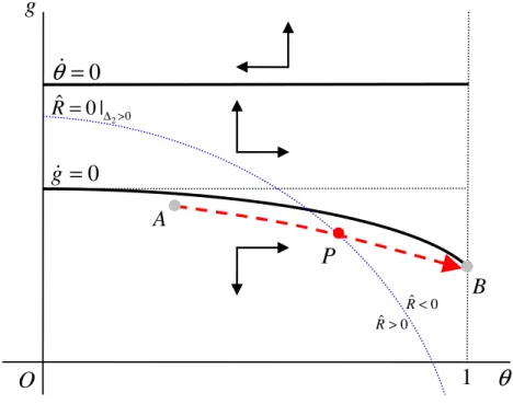
We further examine the dynamics of the RUO regime in the phase diagram in (θ, g)-space as shown in Figure 1. The income share locus ˙θ= 0 represents (27) and gives combinations ofθ and g for which the energy income share is constant. There is a unique innovation rate that leads to a constant energy income share, so that the income share locus is horizontal at this specific value ofg. Intuitively, the growth rates of the effective prices of intermediate goods and energy are equal along the ˙θ= 0 line, leading to constant income shares. At points below the income share locus, the effective price of energy relative to the intermediate goods increases (r−wˆ+νg >0), so that the income share of energy rises over time andvice versa. The dynamic behavior ofθis illustrated by the horizontal arrows in the phase diagram.11

The innovation locus ˙g= 0 represents (28) and gives combinations ofθandgfor which the innovation rate is constant over time. The ˙g= 0 line is downward sloping, because an increase inθ leads to a lower real interest rate (see (31)) and therefore to slower output growth. As a result,K tends to decrease over time, which induces a flow of labor from the production to the research sector, causing the innovation rate to rise over time. To counteract this effect,g

11

Figure 1: Phase diagram in (θ, g) space: RUO regime

O

0

g

=

0

θ

=

g

θ

1

ˆ 0 |

R

=

•

•

B

A

•

P

Notes: The dashed arrow represents the unique equilibrium path that leads to point B, governed by the dynamic system forθandg. The solid lines represent the isoclines forθandg. The dotted line gives the extraction isocline.

must decrease thereby enhancing the growth rate of labor demand as a result of its combined effect on output growth (through the real interest rate) and the productivity of the factors of production. At points to the right of the innovation locus, the real interest rate and output growth are lower than in steady state equilibrium, so thatK declines and the innovation rate increases over time and vice versa. The dynamic behavior of g is illustrated by the vertical arrows in the phase diagram.

The extraction isocline ˆR= 0 represents (30) and gives combinations ofθandgfor which extraction growth equals zero. The ˆR = 0 line is downward sloping, because a decrease in θ

boosts the real interest rate and therefore the growth rates of output and resource demand. To counteract this effect,g must increase to slow down the growth of resource demand through its combined effect on the real interest rate and the efficiency of resource extraction. At points to the right of the ˆR= 0 isocline, the real interest rate and therefore output growth are lower than required for constant extraction, so that extraction growth becomes negative andvice versa.

Because it will affect the dynamics of the model, it is important to determine the relative positions of the three lines in the phase diagram. First, given thatν >0, the innovation locus (28) cannot intersect the income share locus (27) and the former is always located below the latter in (θ, g)-space. Second, comparing (27) and (30), it is clear that the extraction isocline cannot intersect the income share locus either. Furthermore two important boundary properties of the extraction isocline are given by:

lim θ→1g|Rˆ=0 =−∞, g|Rˆ=0 |_θ=0 =g|_θ˙₌₁− ρ (1−σ)(1 +δ).

Finally, to determine the relative position of the extraction isocline and the innovation locus, we define the following differences:

∆1 ≡ g|_Rˆ₌₀ |θ=0−(g|g˙=0)|θ=1= 1−β β L a[1−β(1 +δ)]−ρ h 1 1−σ −2β(1 +δ) i (1 +δ) [1−β(1 +δ)(1−σ)] , ∆2 ≡ g|_Rˆ₌₀ |_θ=0−(g|_g˙=0)|_θ=0 = 1−β β L a 1−β(1 +δ) 1 +δ −ρ 1−β(1 +δ)(1−σ) (1 +δ)(1−σ) .

If ∆1<0, the extraction isocline is located entirely below the innovation locus and if ∆2 >0, both lines intersect exactly once. The signs of the ∆’s depend crucially on the elasticity of substitution between intermediate goods and energy: limσ→1∆1 = −∞ and ∆2|σ=0 > 0. Hence, the extraction isocline will intersect the innovation locus if σ is small and will be located below it if σ is high. Figure 1 shows the scenario in which ∆2 >0.

Without the existence of a backstop technology, the RUO regime lasts forever and the economy converges along the stable manifold from point A to point B in Figure 1.12 _This equilibrium path is characterized by an ever decreasing innovation rate and an income share of energy that converges to unity. Resource extraction can only increase temporarily and peaks when the economy crosses point P in Figure 1 if ∆2>0. When ∆1 <0, the extraction isocline is located below the saddle path and resource extraction will be decreasing over the entire time horizon. Figure 1 depicts the peak-oil scenario.

When the existence of a backstop technology is taken into account, the economy does not converge to point B and will eventually shift to another dynamic regime. The end point (g, θ) in the phase diagram of the RUO regime now depends on the relative price of the backstop

12

Appendix A.5 shows that point B in figure 1 is the only attainable steady state of the model without a backstop technology that satisfies the transversality condition (20).

technology and intermediate goods and on economic conditions in the subsequent regimes, which will be described below.

3.2 Regime 2: Simultaneous Use

The solution to the simultaneous use (SU) regime is characterized by a constant income share of energy and a closed-form differential equation for the innovation rate, which are both given in Proposition 2.

Proposition 2 In the SU regime, the income share of energy θremains constant at its right after switching’ (RAS) value and equal to13

θ₂+= " η β 1−σ 1−θ¯ ¯ θ σ + 1 #−1 (32)

The innovation rate is decreasing over time, according to the following differential equation

˙

g=−g(νg+ρ). (33)

Proof. See Appendix A.6.

Intuitively, as long asθ < θ+₂, the resource is relatively cheaper than the backstop technology so that only the resource will be used for energy generation. If θ = θ+₂, effective prices of the resource and the backstop technology are equal, which enables a regime of simultaneous use as long as θ remains constant. The declining innovation rate follows from the constant energy and intermediate goods income share during the simultaneous use regime. A constant income share together with relatively intermediates-augmenting technical change (ν > 0) namely implies that the price of intermediate goods should grow faster than the interest rate:

r−wˆ =−νg <0. As a result, K goes down over time, because ˆK =r−wˆ−ρ=−νg−ρ. According to (15),g consequently needs to decline in order to keepθ constant over time, i.e. to ensure thatr−wˆ =−νg <0 remains satisfied.

13_{We use the conventional shortcut notationx}+

j ≡limt↓Tijxj(t) andx

−

Combining (32) with the production function (1), final output in the SU regime can be written as: Y =Nφ 1−θ¯ 1−θ+_{3 σ}−σ1 K. (34)

Differentiating (34) and using (33) gives the growth rate of final output in the SU regime:

ˆ

Y =δg−ρ,

where the evolution of the innovation rate is described by the differential equation in Proposi-tion 2. Its starting and end point will be determined below by using the matching condiProposi-tions that link the different regimes together.

3.3 Regime 3: Backstop Technology Only

Because of our assumption of Hicks neutral technological progress in this regime, the produc-tion funcproduc-tion reduces to:

Nφh(¯θHσ−σ1 + (1−¯)θK σ−1

σ i_σ−σ₁

. (35)

The solution to the ‘backstop technology only’ (BTO) regime is characterized by the expres-sions for the income share of energy and the innovation rate given in Proposition 3.

Proposition 3 In the BTO regime, the income share of energy θ and the innovation rate g

remain constant at their RAS values, which are given by

θ₃+= θ₂+, (36) g₃+= L a +ρ (1−θ+₃)(1−β)−ρ. (37)

Proof. See Appendix A.7.

Intuitively, Hicks neutral technical change implies a fixed income shares of energy and inter-mediate goods. Given that the resource stock is depleted, innovation is the only remaining investment possibility. The constant income share of intermediate goods implies an

unchang-ing return to innovation, resultunchang-ing in a constant innovation rate over time. Substitution of (3), (32), and (36) into (35), gives an expression for final output in the BTO regime:

Y =Nφ 1−θ¯ 1−θ+_{3 σ−}σ₁ K₃+. (38)

Differentiating the labor market equilibrium (17) and using the constancy ofgandθ, it follows that K is constant too in the BTO regime, so that final output growth is given by:

ˆ

Y = ˆY₃+ =φg+₃.

3.4 Linking the Regimes

We will use the optimality condition (21) to link the different regimes. From the first-order conditions associated with the optimization problem of the households, (21) implies that consumption should be continuous at regime shifts:

Y_ij−=Y_j+. (39)

4

Transitional Dynamics and Regime Shifts

In this section, we construct phase diagrams to describe the transitional dynamics of the model and to characterize the different regime shifts that the economy may experience. We have to examine several scenarios and use backward induction, because the equilibrium path that the economy follows during the a certain regime depends on the characteristics of the subsequent regime.

We assume that the initial resource stock is large enough to ensure that the natural resource is relatively cheap compared to its perfect substitute so that the backstop technology is not competitive yet. Formally, this is the case in the RUO regime whenpHN−ξ> pRN−δ,

which implies

θ(t)< θ+₂ =θ₃+≡θ+. (40)

moment, the economy will move from the RUO regime to another regime of energy generation in which the dynamics are no longer described by the system of differential equations in Proposition 1. Depending on the parameter configuration, there are two possibilities at the end of the RUO regime: (i) the economy shifts to the SU regime, and (ii) the economy shifts to the BTO regime. Because the equilibrium path that the economy follows during the RUO regime depends on the characteristics of the subsequent regime, we will discuss both scenarios in turn.

4.1 From Resource Use Only to Backstop Technology Only

In this scenario, the economy shifts from regime 1 to regime 3 at timeT13, when the following equality holds: pH(T13−)N(T − 13) −ξ_=p R(T13−)N(T − 13) −δ_{. (41)}

By using (41) andξ=φin the first line of the relative demand function (3), we findθ₁₃− =θ+_, which implies that θ is continuous at the regime shift. Substitution of θ+ into (1) gives an expression for output at the very end of the RUO regime:

Y₁₃−= (N₁₃−)φ 1−θ¯ 1−θ+ _σσ₋₁ K₁₃−. (42)

Combining (42) and (38) and using the continuity ofθ and N, the matching condition (39) requires K₁₃− =K₃+. Labor market equilibrium (17) with ω₁₃− = 0 and ω+₃ = 1, allows us to rewrite the matching condition as:

L−ag₁₃− = (1−θ+)β θ+_+β(1−θ+₎ L−ag₃+. (43)

Substitution of (37) for g+₃ and solving (43) for g−₁₃, we find:

g₁₃− = L a −β(1−θ +₎ L a +ρ . (44)

Hence, the innovation rate jumps down at the regime shift to free enough labor for the production of energy with the backstop technology while keepingK =LK unaffected.

Proposition 4 The innovation rate at the switching time T13 jumps down fromg−13 to g+3.

Proof. Subtracting (37) from (44), we find

g₁₃− −g₃+=θ+ L a +ρ >0.

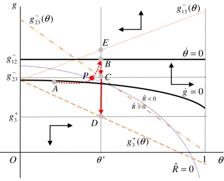
Figure 2 shows the end point (θ+, g−₁₃), labeled B, to which the economy converges in the RUO regime. The equilibrium path that leads to this end point is indicated by the dashed arrow. Along this path, the innovation rate is higher than it would have been in an economy without the backstop technology available (see Figure 1). The figure also contains the extraction isocline and lines for g+₃ and g₁₃− as functions of θ. Note that the end point (θ+, g−₁₃) is located below the ˙θ= 0 line, which is a necessary condition for the regime switch from RUO to BTO to occur.

Figure 2: Phase diagram in (θ, g) space: from RUO to BTO

g

( )

g



B

g



B

A



0

g





g



C

g



O



( )



1



O

1





( )

g



Notes: The dashed arrow represents the unique equilibrium path that leads to point B, governed by the dynamic system forθandg. The solid lines represent the isoclines forθandg. The dotted line gives the extraction isocline. The dotted and dashed lines representg₁₃−(θ) andg₃+(θ), respectively.

inequality should hold:

g₁₃− ≤ φ 1 +δ

L

a. (45)

Proof. By contradiction: If (45) does not hold, the dynamic path in the RUO regime that leads to (θ+, g−₁₃) necessarily intersects the vertical θ+ line before the RUO regime has ended. This would imply that only the resource is being used while the backstop technology is relatively cheaper, which violates optimality of the behavior of final good producers.

Along the equilibrium path in Figure 2, the income share of energy is increasing over time. The innovation rate is initially decreasing, but as soon as the economy crosses the innovation locus, the growth rate starts to increase until the moment of the regime switch. Intuitively, in order to prevent consumption from falling discontinuously when the resource stock is exhausted, the representative household now starts to increase savings when the regime switch comes near. In so doing, the household effectively smooths consumption by converting part of the resource wealth into knowledge, thereby transferring consumption possibilities to the future regime in which the resource stock is depleted. In the figure, resource extraction peaks when the saddle path crosses the extraction isocline at point P and decreases afterwards. However, the extraction path might also be upward sloping during the whole time span of the RUO regime, if it would be located entirely above the equilibrium path.

4.2 From Resource Use Only to Simultaneous Use

If condition (45) is not satisfied, the economy will not experience a sudden shift from a regime in which energy is generated by the natural resource only to an era in which energy generation relies exclusively on the backstop technology. In this case, the shift from the natural resource to the backstop technology occurs more gradually, trough a regime in which both energy sources are used simultaneously.

Figure 3: Phase diagram in (θ, g) space: from RUO to SU

O

0

g

=

0

θ

=

g

θ

1

ˆ 0

R

=

( )

g

θ

θ

g

( )

g

θ

B

A

C

D

•

g

( )

g

θ

P

•

g

•

E

•

•

•

Notes: The curved dotted arrow represents the unique equilibrium path of the RUO regime that leads to point B, governed by the dynamic system forθandg. The straight dotted arrow shows the equilibrium path of the SU regime, leading to point C. The solid arrow represents the jump from point B to C at the end of the SU regime. The solid lines represent the isoclines forθandg. The dotted line gives the extraction isocline. The dotted, dash-dotted, and dashed lines representg₁₃−(θ),g₂₃−(θ), andg₃+(θ), respectively.

regime: Y₁₂−= (N₁₂−)φ 1−θ¯ 1−θ+ _σσ₋₁ K₁₂−. (46)

Combining (34) and (46) and using the continuity ofθ and N, the matching condition (39) requires K₁₂− = K₂+. Together with the labor market equilibrium (17) with ω−₁₂ = 0, this equality implies: L−ag₁₂− = (1−θ +_)β ω₂+θ+_{+ (1−θ}+_)β L−ag + 2 . (47)

We derive a relationship between ω andg in the SU regime by substituting the labor market equilibrium (17) into the innovation return equation (15) noting that r−wˆ =−νg:

ω = [L(1−β)−ag(1−βν)] (1−θ)

Using this relationship to substitute forω₂+ in (47), the matching condition reduces to

L−ag₁₂− = a

φ(1−ν)g

+

2 . (49)

This matching condition implies that the innovation rate is continuous at timeT12, when the economy shifts from regime 1 to regime 2.

Proposition 6 The innovation rate at the switching time T12 is continuous and equal to:

g₁₂− =g₂+= φ 1 +δ

L

a. (50)

Proof. The innovation rateg₁₂− cannot exceedφ/(1+δ)(L/a), because otherwise the dynamic path in the RUO regime necessarily intersects the verticalθ+ line before the RUO regime has ended. This would imply that only the resource is being used while the backstop technology is relatively cheaper, which violates optimality of the behavior of final good producers. Given thatω≥0, it follows from (48) that the innovation rateg+₂ also cannot exceedφ/(1+δ)(L/a). Consequently, the only solution to (49) is given by equation (50) in Proposition 6.

Figure 3 shows the end point (θ₁₂−, g−₁₂), indicated by B, and the equilibrium path towards it in the RUO regime before the switch to simultaneous use takes place. Hence, the economy moves from point A to point B in the figure. Point E cannot be reached, because of the argument provided in the proof of Proposition 6. The income share of energy increases over time, while the innovation rate again exhibits a non-monotonic time profile: it decreases initially but starts to increase once the economy has passed the innovation locus. The saddle path necessarily crosses the extraction isocline, so that resource extraction peaks at point P and decreases afterwards.

The existence of a simultaneous use regime depends on the costs and revenues of innovation (i.e., on a and β) and on the costs of the backstop technology, (i.e., on η). If innovation revenues would be zero (i.e, if β = 1 or a→ ∞), there would be no investment in R&D at all. Without investment in R&D, there necessarily exists a regime of simultaneous use. The reason is that in this scenario resource use has to decline gradually to zero, in order to prevent a jump in marginal utility. Near the regime shift, the marginal product of energy would be very high if all labor would remain in the production sector. Therefore, in the equilibrium

labor starts to flow from the intermediate goods sector to the backstop sector before the shift to the backstop era. Simultaneous use is the only way to smooth consumption by shifting part of the resource wealth to the future. Accordingly, savings behavior of the households ensures that the interest rate is equal to the growth rate of the backstop price. In a market equilibrium with positive R&D (whenβ <1 anda ∞), households have an additional way to smooth consumption. In scenarios with profitable innovation possibilities and a relatively cheap backstop technology, consumption smoothing may completely take place through this new channel: simultaneous use will not occur. If, however, innovation is less profitable, or the backstop technology is relatively expensive so that it will absorb a substantial amount of the labor supply after the regime switch, part of the consumption smoothing still takes place through a temporary regime of simultaneous use, during which the production of the backstop technology starts from zero at the beginning of this regime and gradually increases to its mature long-run level.

4.3 From Simultaneous Use to Backstop Technology Only

Combining (34) and (38), and using the continuity ofθ and N, the matching condition (39) requires K₂₃− = K₃+. Together with the labor market equilibrium (17) with ω₃+ = 1, this equality implies: (1−θ+)β ω₂₃−θ+_{+ (1−θ}+_)β L−ag − 23 = (1−θ +_)β θ+_{+ (1−θ}+_)β L−ag + 3 .

Substitution of (48) forω₂₃− on the left hand side and (37) forg₃+on the right hand side, gives an expression for the innovation rate at the end of the SU regime:

g₂₃− = (1−β)(1−θ)(L+aρ)

a(1−ν) >0, (51)

where the inequality follows fromν <1, which is required for the SU regime to exist.14

Proposition 7 The innovation rate at the switching time T23 jumps down fromg−23 to g+3.

14

The SU regime can only exist if theg−13line in Figure (3) intersects the income share locus, which requires ν <1.

Proof. Subtracting (37) from (51), we find:

g₂₃− −g₃+= Lν(1−β)(1−θ) +a[1−ν+ν(1−β)(1−θ)]ρ

a(1−ν) >0.

The evolution of the innovation rate fromg+₂ tog₂₃− during the SU regime and the jump from

g₂₃− to g₃+ at T23 are indicated by the dashed arrow from point B to point C and the solid arrow from point C to point D in Figure 3, respectively. The figure also contains a line for

g₂₃− as a function of θ.

By using the expenditure share definition (4), the Hotelling rule (23), the backstop price (9), and ˆE = ˆK =−νg−ρ, we find the growth rate of resource extraction:

ˆ

R =− ω

1−ωωˆ−ρ=−

ν(1−β)(1−θ)L+a[1−ν+ν(1−β)(1−θ)]ρ aθ(1−ν)(1−ω) <0,

where the last equality uses (48) and the labor market equilibrium (17). Hence, resource extraction decreases over time during the SU regime.

5

Initial Conditions

To determine the initial value for the energy income share θ, we exploit the fact that total resource extraction over time should be equal to the initial resource stock. We derive a differential equation for the stock rate y ≡ S/R in terms of y, θ and g. Together with the already determined saddle path in (θ, g)-space, the differential equation for the stock rate gives rise to a unique equilibrium path in (θ, y)-space that leads to a zero stock rate at the moment of the switch to the BTO regime (i.e. at t=Ti3). Then, we use the relative factor demand function and the function g = f(θ), which is defined by the saddle path in (θ, g )-space, to derive a relationship between the initial θ and y. The initial income share θ then follows from the intersection of the equilibrium path and the initial relative factor demand function in (g, y)-space. We study the scenarios with and without simultaneous use in turn.

5.1 No Simultaneous Use

If the economy shifts from the RUO to the BTO regime without an intervening period of simultaneous use, the stock rate should equal zero at the end of the RUO regime. The first

row in the relative factor demand function (3) can be written as: θ 1−θ = ¯ θ 1−θ¯ yKNν S 1−_σσ . (52)

Converting (52) into growth rates, we obtain

ˆ θ= (1−θ)1−σ σ ˆ K+νg+ ˆy−Sˆ .

By using (A.12), (A.14) and ˆS =−y−1, we get the differential equation for y in terms of y,

θ, andg: ˙ y =−y(1−θ)(1−σ) φL a −(1 +δ)g +yρ−1. (53)

Imposing the end point y(T₁₃−) = 0 and using the already determined time paths of θ and

Figure 4: Determining the Starting Point

O

y

θ

1

B

•

A

•

(0)

θ

(0)

y

θ

Notes: The dashed arrow represents the unique equilibrium path that leads to point B, governed by the dynamic system forθ, g and y. The solid line gives the relationship between θ(0) and y(0) according to the relative factor demand equation (52) usingg=f(θ).

g, the differential equation (53) yields a unique equilibrium path for y in (θ, y)-space. By plugging the initial stocksN0 andS0into (52) and using the labor market equilibrium (17) to substitute forK, we obtain a second relationship betweenθand y. A combination of the two

relationships yields the starting point [θ(0), y(0)] that is consistent with complete depletion of the resource stock. The starting point corresponds with point A in Figure 4, where the dashed arrow represents the unique equilibrium path that leads to point B, governed by the dynamic system for θ, g and y, and the solid line gives the relationship between θ(0) and

y(0) according to the relative factor demand function. The dynamic behavior of θ and y is illustrated by the horizontal and vertical arrows, respectively.

5.2 Simultaneous Use

If the economy shifts from the RUO to the SU regime, the stock rate should be strictly positive at the beginning of the SU regime. Because of the continuity of relative factor prices and the innovation rate atT12, the stock rate should also be continuous atT12, i.e. y12− =y

+ 2. To determine the value of the stock rate at T12, we exploit the equilibrium condition that total extraction in the SU regime should be equal to the remaining stock at the beginning of this regime. Analogous to the derivation of (53) we use the relative demand equation (3) to obtain a differential equation for the stock rate in terms ofy and ω:

˙

y = ν(1−β)(1−θ) +a[1−ν+ν(1−β)(1−θ)]ρ

aθ(1−ν)(1−ω) y−1,

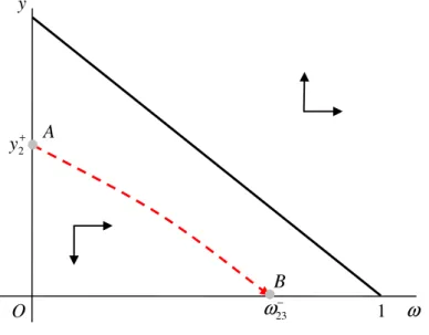
Together with the time path forω, this differential equation for the stock rate gives rise to a unique equilibrium path in (ω, y)-space that leads to a zero stock rate at the moment of the switch to the BTO regime (i.e. at t = T23). The stock rate at the switching moment then follows by evaluating y along this equilibrium path in (ω, y)-space at ω+₂ = 0. This point corresponds with the vertical intercept A of the dashed arrow in Figure 5. The solid line in the figure gives combinations ofω and y for which the stock rate is constant over time. The dynamic behavior ofω andyis illustrated by the horizontal and vertical arrows, respectively. Having determined y₁₂− = y₂+, as before we can use (53) to construct the unique path leading to this stock rate at the end of the RUO regime, which together with (52) yields the start point [θ(0), y(0)], labeled A in Figure 6. The dashed arrow in the figure shows the equilibrium path leading to (θ+, y₁₂−) indicated by B, and the solid line depicts the relationship between the start valuesθ(0) andy(0).

Figure 5: Determining the Stock Rate at the Regime Switch O y

ω

ω

•

•

Notes: The dashed arrow represents the unique equilibrium path that leads to point B, governed by the dynamic system forωandy. The solid line is the ˙y= 0 locus, which gives combinations ofωandysuch thatyis constant over time.

Figure 6: Determining the Starting Point

O

y

θ

1

B

•

A

(0)

θ

(0)

y

y

θ

•

Notes: The dashed arrow represents the unique equilibrium path that leads to point B, governed by the dynamic system forθ, g and y. The solid line gives the relationship between θ(0) and y(0) according to the relative factor demand equation (52) usingg=f(θ).

6

Numerical Illustration

In this section, we perform a simulation analysis to quantify the transitional dynamics of the model. We investigate two scenario’s: one benchmark in which simultaneous use of the resource and the backstop technology occurs for a considerable period of time and one alternative scenario in which the economy switches abruptly from the resource to the backstop technology without an intermediate era of hybrid energy generation. As a robustness check, we also provide simulation results for a formulation of our model in which the resource and the backstop technology are good instead of perfect substitutes.15 We first calibrate the model and then present the simulation results.

6.1 Calibration

There is ample evidence that the elasticity of substitution between energy and man-made factors of production is less than unity. Koetse, de Groot, and Florax (2008) conduct a meta-analysis and find a point estimate for the cross-price elasticity between capital and energy in Europe of 0.338 in the short run and 0.475 in the long run. We take the average of these values to obtain σ = 0.4. According to the estimation results of Roeger (1995), the markup of prices over marginal cost in the manufacturing sector of the U.S. economy over the period 1953-1984 varied from 1.15 to 3.14. To cover this range, we imposeβ= 0.8 in our benchmark scenario andβ = 0.3 in the alternative scenario.16 We set the production function parameter

¯

θ and the rate of pure time preferenceρ to 0.1 and 0.01, respectively. By imposing δ= 0.05, we ensure that knowledge spillovers to the resource extraction sector are small. Labor supply

L and the initial knowledge stock N0 are normalized to 1 and 0.1, respectively.

The initial resource stock is chosen such that the initial share of resource expenditures in GDP θ0 equals 8.8 percent, to match the average US energy expenditure share in GDP over the period 1970-2009 (U.S. Energy Information Administration, 2012). We use the research productivity parameter a to obtain an initial consumption growth rate ˆC0 of 1.7 percent, which is equal to the average yearly growth rate of GDP per capita in the US over the period 1970-2010 (The Conference Board, 2011). Our benchmark calibration implies an initial reserve to extraction rate of y0 = 52, being close to the global proved oil reserves to oil production

15

For the substitution elasticity between the resource and the backstop technology, we chooseγ= 50. 16_{In the alternative scenario, we adjustaandηto keep initial consumption growth andθ}+_unchanged.

ratio in 2011 reported in BP (2012). Initially, the ratio between the per unit of energy price of the backstop technology and the resource,pH0/pR0N₀−ν, amounts to 3. In both scenarios, the current era in which energy generation relies on the non-renewable resource ends in roughly 4 decades.

6.2 Results

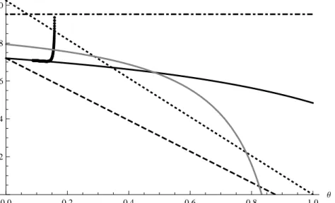
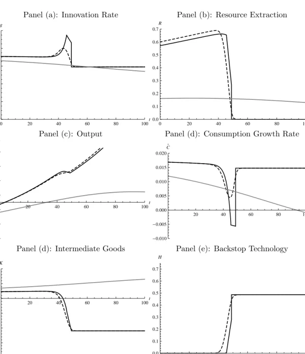
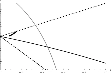
Benchmark Calibration Figure 7 contains the phase diagram for the benchmark calibra-tion and corresponds with Figure 3, which sketches the general case as discussed in Seccalibra-tion 4.2. The fat dotted stable manifold starts just below the solid innovation locus, crosses the gray extraction isocline at the moment of peak-oil, and reaches the dash-dotted income share locus at the moment the economy switches to the simultaneous use regime. Accordingly, the innovation rate first decreases slightly over time, but starts to increase after the stable manifold has crossed the innovation locus. During the simultaneous use regime, the innovation rate declines gradually to the dottedg₂₃−(θ) line and then jumps down to the dashed g₃+(θ) line. This jump marks the beginning of the backstop technology only regime, during which the innovation rate remains constant over time.

Figure 7: Phase Diagram (Benchmark Scenario)

0.0 0.2 0.4 0.6 0.8 1.0 Θ 0.02 0.04 0.06 0.08 0.10 g

Notes: The solid and dash-dotted line represent the innovation locus and income share locus, respectively. The fat dotted path represents the stable manifold. The gray line is the extraction isocline. The dashed and the dotted line represent theg+₃(θ)-line and the g−₂₃(θ)-line, respectively. The underlying parameters values are: a= 2.5,β = 0.8,

The solid line in Panel (a) of Figure 8 depicts the time path of the innovation rate in accordance with the analysis of the phase diagram in Figure 7. To illustrate the importance of taking the backstop technology into account, the gray line shows the innovation rate in a world similar to the benchmark economy, but without the availability of a backstop technology. In contrast to the benchmark case, innovation in such a world decreases monotonically over time and starts out lower. As a robustness check, the dashed line represents the time path in a model in which the resource and the backstop technology are good, but imperfect substitutes. The imperfect substitutes model yields time paths that, though smoother and with less pronounced extrema, are quite similar to those generated by our simpler model in which the resource and the backstop technology are perfect substitutes.

Panel (b) shows that extraction is increasing initially, peaks just before the economy switches to the simultaneous use regime and decreases subsequently until the stock is ex-hausted. Due to the finite exhaustion time, extraction starts out considerably higher than in the model without a backstop technology. Panels (c) and (d) depict output and its growth rate, respectively. Output growth is positive initially and in the long run, but becomes negative temporarily during the run-up to the introduction of the backstop technology. Consumption growth is decreasing over time during the first two regimes and then jumps up to a constant rate in the backstop technology only regime. Conversely, consumption growth is monotonically decreasing over time and eventually becomes negative in the model without a backstop technology.

As shown in Panel (d), the input of intermediate goods declines significantly during the end of the resource use only regime, to make free labor for backstop technology production. This effect is absent in the model without a backstop technology, resulting in an upward-sloping time path of intermediate goods. Backstop technology production is zero until the start of the simultaneous use regime, during which it increases quickly, as shown in Panel (e). At the end of this regime, backstop technology production jumps up to a constant level in the backstop technology only regime.

Alternative Calibration In the alternative scenario (with a larger price markup), the economy immediately jumps from the resource use only to the backstop technology only regime, without an intermediate period of simultaneous use. The phase diagram for the

Figure 8: Transitional Dynamics (Benchmark Scenario)

Panel (a): Innovation Rate Panel (b): Resource Extraction

0 20 40 60 80 100t 0.00 0.02 0.04 0.06 0.08 0.10 g 0 20 40 60 80 100t 0.0 0.1 0.2 0.3 0.4 0.5 0.6 0.7 R

Panel (c): Output Panel (d): Consumption Growth Rate

20 40 60 80 100t 0.0 0.2 0.4 0.6 0.8 1.0 1.2 Y 20 40 60 80 100t -0.010 -0.005 0.000 0.005 0.010 0.015 0.020 C`

Panel (d): Intermediate Goods Panel (e): Backstop Technology

20 40 60 80 100t 0.60 0.65 0.70 0.75 0.80 0.85 0.90 K 0 20 40 60 80 100t 0.0 0.1 0.2 0.3 0.4 0.5 0.6 0.7 H

Notes: The solid line represents scenario 1, in which a backstop technology that provides a perfect substitute for the resource is available. The gray line represents scenario 2, in which there is no backstop technology available. The dashed line represents scenario 3, in which a backstop technology that provides a good, but imperfect substitute for the resource is available. Parameters are set to: a= 2.5,β= 0.8,δ= 0.05,η= 3,ρ= 0.01,σ= 0.4, ¯θ= 0.9, ¯ω= 0.1,

γ= 50,L= 1. The initial knowledge stockN0 equals 0.1. The initial resource stockS0equals 30 in scenario 1 and 2

to obtainθ0= 0.088 in scenario 1. In the third scenario, the initial resource stock in the third scenario is chosen such

Figure 9: Phase Diagram (Alternative Scenario) 0.0 0.2 0.4 0.6 0.8 1.0 Θ 0.002 0.004 0.006 0.008 0.010 0.012 0.014 g

Notes: The solid line represents the innovation locus. The fat dotted path represents the stable manifold. The gray line is the extraction isocline. The dashed and the dotted line represent theg+₃(θ)-line and theg−₁₃(θ)-line, respectively. The underlying parameters values are: a= 65,β= 0.3,δ= 0.05,η= 1.125,ρ= 0.01,σ= 0.4, ¯θ= 0.9, ¯ω= 0.1,γ= 50,

L= 1.

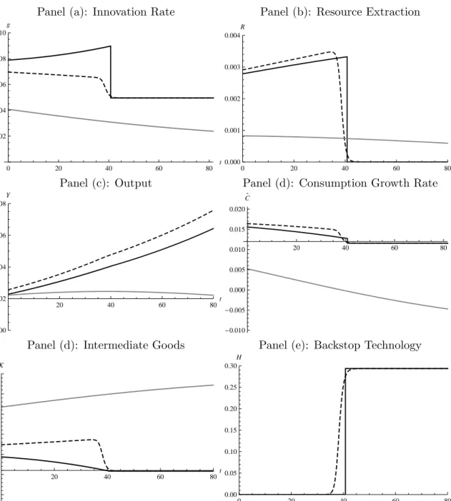
alternative calibration is shown in Figure 9, corresponding to the general case discussed in Section 4.1 and shown in Figure 2. The fat dotted stable manifold now starts above the innovation locus and does not intersect the gray extraction isocline. Hence, both the innovation rate and resource extraction are increasing over time until the end of the resource use only regime has been reached as the stable manifold hits the dotted g₁₃− line. The energy income share now remains constant at θ+ and the innovation rate jumps down to the corresponding constant value at the dashed g₃+ line. This jump marks the beginning of the backstop technology only regime.

Figure 10 shows the transitional dynamics for the alternative calibration. Besides the absence of a simultaneous use regime, the most important differences are that the innovation rate and resource extraction are and remain increasing over time until the resource stock is exhausted, as shown in Panels (a) and (b).17 _{Furthermore, Panels (c) and (d) reveal} that the temporarily negative consumption growth has disappeared. Finally, there are some

17

Because the run-up to the backstop technology has already begun att= 0 (the stable manyfold starts above the innovation locus), there is a discrepancy between the initial innovation rate in the perfect and imperfect substitutes model. When we decreaseθ0far enough, this discrepancy disappears as in the benchmark scenario shown in Figure 8.

Figure 10: Transitional Dynamics (Alternative Scenario)

Panel (a): Innovation Rate Panel (b): Resource Extraction

0 20 40 60 80 t 0.002 0.004 0.006 0.008 0.010 g 0 20 40 60 80t 0.000 0.001 0.002 0.003 0.004 R

Panel (c): Output Panel (d): Consumption Growth Rate

20 40 60 80t 0.000 0.002 0.004 0.006 0.008 Y 20 40 60 80 t -0.010 -0.005 0.000 0.005 0.010 0.015 0.020 C`

Panel (d): Intermediate Goods Panel (e): Backstop Technology

20 40 60 80t 0.3 0.4 0.5 0.6 0.7 0.8 0.9 K 0 20 40 60 80t 0.00 0.05 0.10 0.15 0.20 0.25 0.30 H

Notes: The solid line represents scenario 1, in which a backstop technology that provides a perfect substitute for the resource is available. The gray line represents scenario 2, in which there is no backstop technology available. The dashed line represents scenario 3, in which a backstop technology that provides a good, but imperfect substitute for the resource is available. Parameters are set to: a= 65,β= 0.3,δ= 0.05,η= 1.125,ρ= 0.01,σ= 0.4, ¯θ= 0.9, ¯

ω = 0.1,γ = 50,L= 1. The initial knowledge stock N0 equals 0.1. The initial resource stockS0 equals 0.125 in

scenario 1 and 2 to obtain θ0 = 0.088 in scenario 1. In the third scenario, the initial resource stock in the third

but no significant deviations from the benchmark scenario in the time paths for man-made inputs (Panels (d) and (e)): intermediate goods input now declines over time until the backstop technology is introduced and remains constant afterwards, and backstop technology production jumps up from zero to a constant positive number at the switching instant.

7

Conclusion

We have investigated the effects of the availability of a backstop technology on the time paths of resource extraction and the rate of technological progress, taking into account that natural resources and man-made inputs are poor substitutes and that generation of energy with the backstop technology is costly. To this end, we introduce a non-renewable resource and a backstop technology in a simple general equilibrium endogenous growth model. The elasticity of substitution between energy and man-made inputs is assumed to be smaller than unity. The backstop technology can be used to produce a perfect substitute for the natural resource. Technological progress is driven by workers in R&D, who build upon previously generated knowledge. We solve the model analytically and develop a graphical apparatus to visualize its transitional dynamics and regime shifts. Moreover, we quantify the results by calibrating the model and performing a simulation analysis. The results are robust to relaxing the assumption of perfect substitutability between the resource and the backstop technology. Our main findings can be divided into four categories: energy regimes, technological change, resource extraction, and reserve to extraction ratio. Regarding the first category, we find that the economy experiences different regimes of energy generation. Initially, the economy relies exclusively on the natural resource. In the long run, the natural resource will be abandoned in favor of the backstop technology. In between these two regimes, depending on parameter values, there may exist an intermediate era during which the resource and the backstop technology are used simultaneously. This feature is noteworthy, because the model does not impose the convexities in resource extraction or backstop production costs that are normally required to obtain this result.

Second, the introduction of a backstop technology in the model crucially affects the shape of the time path of technological progress, measured by the rate of innovation. Instead of monotonically decreasing as it would be without the backstop technology, the rate of innovation exhibits a non-monotonic development over time: it first decreases gradually, but

during the run-up to the introduction of the backstop technology it starts to increase in order to prevent a downward jump in consumption at the time of the shift to the backstop regime. Once the economy enters the backstop regime, the rate of innovation jumps down to its long-run value to free resources for production in the backstop sector. At any moment during the resource regime, the rate of innovation is strictly higher than it would be without the availability of a backstop technology.

Third, the introduction of the backstop technology has notable implications for the de-velopment of resource extraction over time. The resource extraction path does no longer eventually have to become downward-sloping. Depending crucially on the bias in techno-logical change and the elasticity of substitution between energy and man-made inputs, the extraction path can be monotonically upward-sloping or downward sloping until exhaustion, or exhibit an internal maximum, known as ‘peak-oil’. Poor substitutability between the natural resource and man-made inputs, and technological change that is strongly resource-using lead to increasing resource extraction over time.

Fourth, while the calibrated model with the backstop technology generates a reserve to extraction rate in line with the most recent global figure for crude oil, the specification of the model without the backstop technology implies a reserve extraction rate that is way too high compared with the data. Accordingly, this finding might suggest that resource markets have already priced in the future adoption of backstop technologies, leading to smaller reserve to extraction rates than when the economy is deemed to necessarily rely upon the natural resource forever.

The most important direction for further research is the introduction of pollution from combustion and stock-dependent costs of extraction of the natural resource. In combination with the backstop technology these features make it interesting to compare the decentralized outcome to the social optimum, in order to shed light on optimal environmental policy. Another useful extension of the current analysis would be the introduction of separate R&D activities for man-made-inputs-augmenting and energy-augmenting technological change, so that the bias in technological progress becomes endogenous.

Appendix

A.1 Final Output

In this section, we derive the relative factor demand equation (3). Profits of firms in the final output sector are given by:

pY  θE¯ σ−1 σ + (1−θ¯) Z N 0 k_jβdj σ −1 βσ   σ σ−1 − Z N