Fast Automatic Segmentation of the Esophagus
from 3D CT data using a Probabilistic Model
Johannes Feulner1,3, S. Kevin Zhou2, Alexander Cavallaro4, Sascha Seifert3, Joachim Hornegger1,5, and Dorin Comaniciu2
1 Chair of Pattern Recognition, University of Erlangen-Nuremberg, Germany, [email protected],
2 Siemens Corporate Research, Princeton, NJ, USA 3
Siemens Corporate Technology, Erlangen, Germany
4 Radiology Institute, University Hospital Erlangen, Germany 5
Erlangen Graduate School in Advanced Optical Technologies (SAOT), Germany
Abstract. Automated segmentation of the esophagus in CT images is of high value to radiologists for oncological examinations of the medi-astinum. It can serve as a guideline and prevent confusion with patho-logical tissue. However, segmentation is a challenging problem due to low contrast and versatile appearance of the esophagus. In this paper, a two step method is proposed which first finds the approximate shape using a “detect and connect” approach. A classifier is trained to find short seg-ments of the esophagus which are approximated by an elliptical model. Recently developed techniques in discriminative learning and pruning of the search space enable a rapid detection of possible esophagus segments. Prior shape knowledge of the complete esophagus is modeled using a Markov chain framework, which allows efficient inferrence of the approx-imate shape from the detected candidate segments. In a refinement step, the surface of the detected shape is non-rigidly deformed to better fit the organ boundaries. In contrast to previously proposed methods, no user interaction is required. It was evaluated on 117 datasets and achieves a mean segmentation error of 2.28mm with less than 9s computation time.
1
Introduction
The mediastinal region is of particular interest to radiologists for oncological examinations [1]. For diagnosis and therapy monitoring, CT scans of the thorax are common practice. Lymphoma, which is the second most common tumor in the mediastinum, often affects regions close to the trachea and the esophagus as these are natural gateways of the human body. While the trachea is very easy to see in CT, the esophagus is sometimes hard to find in single slices. Especially in coronal view, even experts have difficulties to see the boundaries, which is one reason why interpretation of the images is tedious. Fast and automatic seg-mentation of the esophagus can shorten the time a radiologist needs to read an image.
Automated segmentation of the esophagus is challenging because of its com-plex shape and its inhomogeneous appearance. As its wall consists of muscle
tissue, there is only little contrast if it is empty. Sometimes it is filled with air bubbles, remains of oral contrast agent or both. Up to now, there are few publi-cations on esophagus segmentation, and all of them require a significant amount of user input. In [2], a probabilistic spatial and appearance model is used to ex-tract the centerline. In a second step, the outer wall is approximated by fitting an ellipse into each slice using a region-based criterion. However, the method requires as input two points on the esophagus and furthermore a segmentation of the left atrium and the aorta. In [3], a semi-automated method is proposed that takes one contour in an axial slice as user input and propagates the contour to other slices by registration using optical flow. The quality of the segmentation was not evaluated quantitatively. Another semi-automated method is described in [4]. The user draws several contours in axial slices. The segmentation is ob-tained by interpolating the contours in the frequency domain. The image itself is not used.
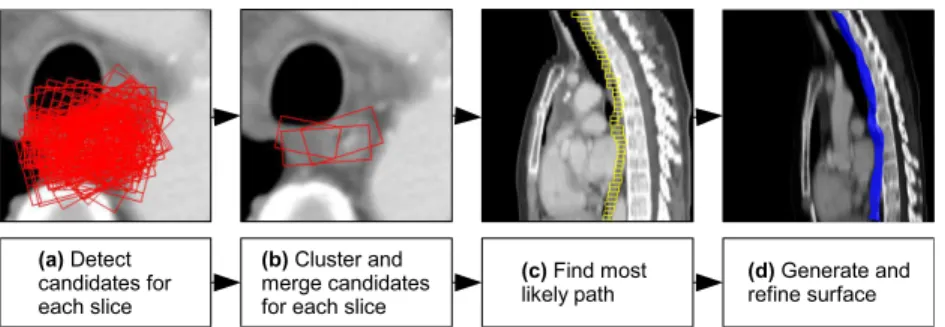
In this work, a method is proposed that first detects the approximate shape. This is carried out in three sub steps, which are visualized in Figure 1 (a-c). In step (a), for each slice a detector that was trained from annotated data is run to detect weighted candidate esophagus segments, which are modeled as ellipses. An ellipse in visualized by its bounding box. These candidates are clustered to find modes in the distribution (b). Candidates of a cluster are merged into a weighted cluster center. A Markov chain model is then used to find the most likely path through the cluster centers. Prior shape knowledge is incorporated into the Markov chain by learning the transition probability distribution from a slice to the next from annotated data. In the final step (d), a surface is generated from the detected sequence of ellipses. A detector is trained offline to learn the boundary of the esophagus. The surface is deformed along its normals and smoothed to adapt the mesh to the organ boundary.
2
Esophagus segmentation
2.1 Ellipse detection
To approximate the contour of the esophagus, an elliptical model was chosen as it can be described by a relatively low dimensional parameter vectore
e= (x, y, θ, a, b) (1)
where x and y are the coordinates of the center within an axial slice, θ is the rotation angle andaandb are the semi-major and the semi-minor axis, respec-tively.
Recently developed techniques in discriminative learning [5] and search space pruning based on learning in marginal spaces [6] enable a rapid detection of can-didate model instances. A probabilistic boosting tree (PBT) classifier was trained with a large number of positive and negative examples to learn the target distri-bution p(m= 1|e,v) which describes the probability that eis a correct model instance in the currently observed imagev. In order to accelerate search, a de-tector was also trained on the subspaces (x, y) and (x, y, θ) of the full parameter space e to learn the distributions p(m= 1|(x, y)) andp(m= 1|(x, y, θ)). This allows to reject wrong model instances at an early stage. As feature pool, a com-bination of 3D Haar-like and steerable features were used [6]. Haar-like features are computed by convolving the image with box filter kernels of different size, position and weight. They gain their power from speed as they can be computed in constant time even for large kernels using an integral image. They are called Haar-like because of their similarity to the Haar wavelets. Steerable features are simple point features like intensity and gradient and nonlinear combinations of those evaluated at a certain sampling pattern, which is a regular grid of size 7×7×3 in this case. The final output are the N best model instances e(i), i= 1. . . N together with a scoreς(i)=p(m= 1|e(i),v) for each one.
In order to reduce subsequent search effort and to detect modes in the distri-bution of the candidates, they are clustered using an agglomerative hierarchical average-linkage clustering algorithm until a distance thresholddmax is reached, which was set to 10mm in the experiments. The distribution is now represented by the cluster centers c(1). . .c(K) with weights σ(1). . . σ(K), where the weight σ(k) of cluster centerkis the sum of weights of all members.
2.2 Inferring the path
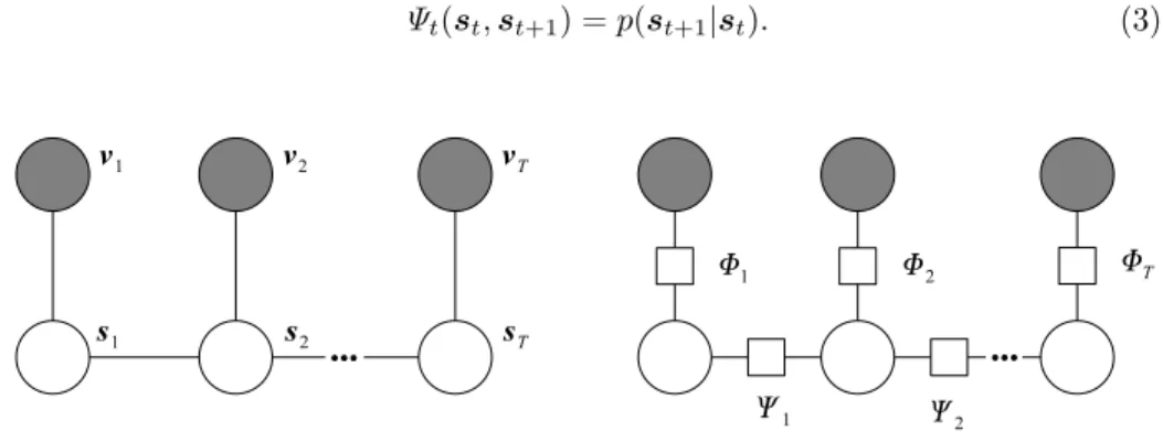
So far, the axial slices of the volume image were treated separately. Shape knowl-edge is incorporated into a Markov chain model [7] of the esophagus, which is used to infer the most likely path through the axial slices. A graph of the Markov model used is depicted in Figure 2 (left). The variabless1. . .sT correspond to the axial slices of the image. Possible states of a variablestare the ellipses cor-responding to the cluster centersc(tk), k= 1. . . Ktof slice t. Each state variable st is conditioned on the observed image slicevt. In Figure 2 (right), the factor
graph [8] of the Markov model is shown. The clique potentials (or factors) of the observation cliques are denoted withΦt. They are set to the score of the cluster
centers: Φt(c (k) t ,vt) =σ (k) t . (2)
The clique potentialsΨt between adjacent state variablesst,st+1 represent the prior shape knowledge. They are set to the transition distribution from one slice to another:
Ψt(st,st+1) =p(st+1|st). (3)
Fig. 2.Markov chain model of the esophagus along with corresponding factor graph.
To simplify the transition distribution, it was assumed that the transition of the translation parameters x, y is statistically independent from the other parameters. The same was assumed for the scale parameters. As the rotation parameterθis not well defined for approximately circular ellipses, the transition of rotation also depends on the scale parameters, but independence was assumed for rotation and translation parameters. With these assumptions, the transition distribution can be factorized and becomes
p(st+1|st) =p(xt+1, yt+1|xt, yt)p(θt+1|θt, at, bt)p(at+1, bt+1|at, bt). (4)
The translation transitionp(xt+1, yt+1|xt, yt) is modeled as a 2D normal
distri-bution N(∆x, ∆y|Σp,mp) and the scale transition p(at+1, bt+1|at, bt) as a 4D
normal distribution N(at+1, bt+1, at, bt|Σs,ms). The variance of the rotation
transition highly increases with the circularity of the ellipse as θ becomes ar-bitrary for a circle. Therefore, p(θt+1|θt, at, bt) is modeled with ten 1D normal
distributions, one for a certain interval of circularity, which is measured by the ratio b a: p(θt+1|θt, at, bt) =N ∆θ σr b a , mr b a . (5)
The parameters of all normal distributions were estimated from manually anno-tated data.
The a posterior joint distribution of all statesp(s1:T|v1:T) is then given by
estimate ˆ s(MAP)1:T = argmax s1:T Φ1(s1,v1) T Y t=2 Φt(st,vt)Ψt−1(st−1,st) ! (6)
can be computed efficiently using the max-sum algorithm, which is a variant of the sum-product algorithm [8].
2.3 Surface generation and refinement
After the MAP estimate of the path has been detected, the sequence of ellipses is converted into a triangular mesh representation by sampling the ellipses and connecting neighboring point sets with a triangle strip.
The cross-section of the esophagus is generally not an ellipse, and the path obtained in section 2.2 often contains some inaccuracies. Therefore, the mesh model is further refined to better fit the surface of the organ.
A PBT classifier was trained to learn the boundary of the esophagus. The classifier uses steerable features as proposed in [6]. As for ellipse detection, the steerable features are sampled on a regular grid, but now with a size of 5× 5×9. For each mesh vertex, the sampling pattern is placed so that the vertex is in the center of the pattern and the longest axis points in direction of the mesh normal. Now the pattern is moved along the normal to find the maximal detector response and the new position of the vertex. Finally, the surface is passed through a Laplacian smoothing filter. This process of deformation and smoothing is repeated for a certain number of iterations.
3
Results
The proposed method was evaluated on 117 CT scans of the thorax using three-fold cross-validation. Manual segmentation was available for each dataset. The spatial resolution of the datasets was typically 0.72×0.72×5mm3. Among the scans, 34 were taken from patients suffering from lymphoma, which often causes enlarged lymph nodes in the mediastinal region. In some datasets, the esopha-gus contained remains of orally given contrast agent. For evaluation, the datasets were cropped around the region of interest.
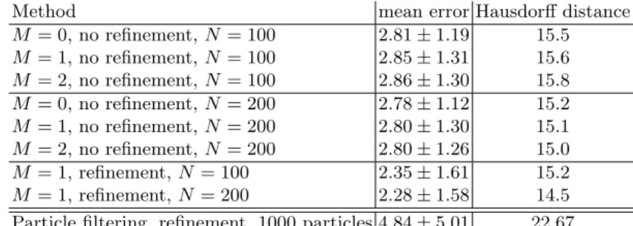
Accuracy: The accuracy of the segmentation was evaluated by comparing the result with the annotated ground truth. Mean mesh-to-mesh distance and Haus-dorff distance (maximal mesh-to-mesh distance) were used as error measures. Results are shown in Table 1. First, results are compared after the path infer-rence step with surface refinement turned off (rows one to six). Accuracy was measured forN = 100 andN = 200 model instance candidatese(i),i= 1. . . N. Additionally to a Markov model with a Markov order of one (M = 1), mea-surements for M = 0 and M = 2 are also included. As a 2nd order Markov chain over some alphabet is equivalent to a first order chain over the alphabet of 2-tuples, the model of Figure 2 was used also for the 2nd order case, but with a state space that consists of 2-tuples and with adapted transition probabilities.
While there is a noticeable improvement withN = 200 compared toN = 100, the Markov order has very little influence on the numerical results. However, the results generated with the Markov model turned on (M = 1 and M = 2) are visually more appealing because they are smooth and look more anatomically reasonable. As M = 1 and M = 2 produce very similar results, M = 1 is proposed as it does not introduce unnecessary complexity. The boundary refine-ment step significantly improves the segrefine-mentation error (rows seven and eight of Table 1). With N = 200 and M = 1, the proposed method gives a mean segmentation error of 2.28mm with a standard deviation of 1.58mm and a mean Hausdorff distance of 14.5mm. For comparison, the path of the esophagus was also detected using a particle filter approach [9] (last row of Table 1). Particle filtering is commonly used for tracking applications and is also becoming popular to detect tubular structures [10, 11]. The Markov chain approach gives consider-ably better results because the image is searched exhaustively and thus it is far less prone to tracking loss.
Method mean error Hausdorff distance
M = 0, no refinement,N= 100 2.81±1.19 15.5 M = 1, no refinement,N= 100 2.85±1.31 15.6 M = 2, no refinement,N= 100 2.86±1.30 15.8 M = 0, no refinement,N= 200 2.78±1.12 15.2 M = 1, no refinement,N= 200 2.80±1.30 15.1 M = 2, no refinement,N= 200 2.80±1.26 15.0 M = 1, refinement,N= 100 2.35±1.61 15.2 M = 1, refinement,N= 200 2.28±1.58 14.5 Particle filtering, refinement, 1000 particles 4.84±5.01 22.67
Table 1.Accuracy of the registration in mm.
Performance: Computation time was measured for the different steps of the algorithm. The results are summarized in Table 2. Time was measured on a 2.2GHz Intel Core2 Duo processor with 2GB of RAM on a volume of size 79× 96×50 voxels. Most of the time is spent on the model detection step, because here the volume is exhaustively searched. Computation time of this step increases linearly with the number N of candidates. In total, segmenting the esophagus takes 3.94s forN = 100 and 8.26s forN = 200.
Method Model detection path inferrence surface refinement total
N= 100 3.67 0.0073 0.26 3.94
N= 200 7.99 0.0069 0.26 8.26
Table 2. The computation time in seconds is shown for the different steps of the algorithm withM= 1.N denotes the number of model candidates.
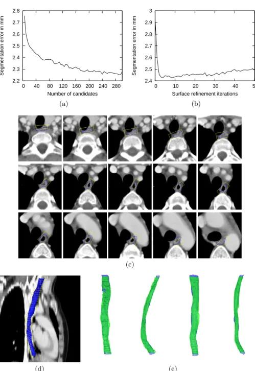
Figure 3 (a-b) shows the segmentation error as a function of the number N of candidates and the number of surface refinement iterations. A value of N = 200 is a good trade-off between accuracy and speed, and two refinement iterations are a reasonable choice. Examples of segmentation results are displayed in Figure 3 (c-e).
2.2 2.3 2.4 2.5 2.6 2.7 2.8 0 40 80 120 160 200 240 280 Segmentation error in mm Number of candidates 2.4 2.5 2.6 2.7 2.8 2.9 3 0 10 20 30 40 50 Segmentation error in mm
Surface refinement iterations
(a) (b)
(c)
(d) (e)
Fig. 3.(a-b): Segmentation error as a function of the numberN of model candidates and the number of surface refinement iterations. (c-e): Examples of segmentation re-sults. The boxes are bounding boxes of ellipses and visualize the inferred approximate shape. The final result after mesh generation and boundary deformation if shown in blue. In (e), the green semitransparent surface is the ground truth segmentation.
4
Discussion
The contribution of this work is twofold. First, the well known MAP framework for Markov chains is combined with the powerful detector based on the PBT clas-sifier with Haar-like and steerable features [6]. Second, the method is extended with a boundary detector and applied to the problem of automatic esophagus segmentation, which is challenging due to the versatile shape and appearance of the organ.
With a mean segmentation error of 2.28mm, the proposed method has a good accuracy. Exhaustive search combined with a Markov model can well han-dle regions with clutter and low contrast. Compared to particle filtering based techniques, it is far less prone to tracking loss. Furthermore the method is fully automatic and very fast with a computation time of 8.3s. It can be easily adapted to other tubular structures like the spinal canal or larger vessels.
In the future we will consider to integrate more prior knowledge into the boundary refinement process. A local model seems most appropriate because otherwise cases where the esophagus is only partially visible cannot be easily handled any more.
References
1. Duwe, B.V., Sterman, D.H., Musani, A.I.: Tumors of the mediastinum. Chest
128(4) (2005) 2893–2909
2. Rousson, M., Bai, Y., Xu, C., Sauer, F.: Probabilistic minimal path for automated esophagus segmentation. Proceedings of the SPIE6144(2006) 1361–1369 3. Huang, T.C., Zhang, G., Guerrero, T., Starkschall, G., Lin, K.P., Forster, K.:
Semi-automated ct segmentation using optic flow and fourier interpolation techniques. Comput. Methods Prog. Biomed.84(2-3) (2006) 124–134
4. Fieselmann, A., Lautenschl¨ager, S., Deinzer, F., John, M., Poppe, B.: Esophagus Segmentation by Spatially-Constrained Shape Interpolation. Bildverarbeitung f¨ur die Medizin (2008) 247–+
5. Tu, Z.: Probabilistic boosting-tree: learning discriminative models for classification, recognition, and clustering. ICCV2(2005) 1589–1596
6. Zheng, Y., Barbu, A., Georgescu, B., Scheuering, M., Comaniciu, D.: Fast auto-matic heart chamber segmentation from 3d ct data using marginal space learning and steerable features. ICCV (2007) 1–8
7. Kindermann, R., Snell, J.L.: Markov Random Fields and Their Applications. AMS (1980)
8. Kschischang, F., Frey, B., Loeliger, H.A.: Factor graphs and the sum-product algorithm. IEEE Transactions on Information Theory47(2) (2001) 498–519 9. Isard, M., Blake, A.: A smoothing filter for condensation. Lecture Notes in
Com-puter Science1406(1998) 767–781
10. Schaap, M., Smal, I., Metz, C., van Walsum, T., Niessen, W.: Bayesian tracking of elongated structures in 3d images. International Conference on Information Processing in Medical Imaging, IPMI (2007)
11. Florin, C., Paragios, N., Williams, J.: Particle filters, a quasi-monte-carlo-solution for segmentation of coronaries. MICCAI (2005) 246–253