The Taxation of Fuel Economy
∗
James M. Sallee
†University of Chicago and NBER
October 5, 2010
Abstract
Policy-makers have instituted a variety of fuel economy tax policies – polices that tax or subsidize new vehicle purchases on the basis of fuel economy performance – in the hopes of improving fleet fuel economy and reducing gasoline consumption. This article reviews existing policies and concludes that while they do work to improve vehicle fuel economy, the same goals could be achieved at a lower cost to society if policy-makers instead directly taxed fuel. Fuel economy taxation, as it is currently practiced, invites several forms of gaming that could be eliminated by policy changes. Thus, even if policy-makers prefer fuel economy taxation over fuel taxes for reasons other than efficiency, there are still potential efficiency gains from reform.
1
Why do we tax fuel economy?
In recent decades, the United States government has introduced several “fuel economy taxes” – that is, taxes or subsidies on the purchase of new consumer automobiles that depend on the vehicle’s fuel economy performance. These policies vary in detail. Some provide subsidies
∗The author would like to thank Jeffrey Brown for editorial guidance and Adam Cole for providing
assistance in locating key data and legislative details.
†Address: James M. Sallee, The Harris School, University of Chicago. Phone: 773-316-3480. Email:
to vehicles that utilize a specific technology (e.g., hybrids), while others apply to all vehicles of a given fuel economy. Some levy taxes directly on automakers, while others operate through the personal income tax system. All attempt to provide automakers and consumers with an incentive to choose more fuel economical vehicles so as to reduce the consumption of gasoline. The purpose of this paper is to review the motivation and structure of these policies, describe their intended and unintended consequences, and distill lessons that may inform future policy.
The principal economic motivation for the taxation of fuel economy is to correct for externalities associated with fuel consumption. Fuel economy itself does not create external-ities, but it indirectly determines the consumption of gasoline, which affects local air quality, energy security and global climate change. The goal of fuel economy taxation is to cause consumers to internalize these externalities by raising the price of fuel inefficiency.
Policies to reduce energy consumption in the personal transportation sector are an essen-tial part of energy policy – the sector accounts for 20% of U.S. greenhouse gas emissions and 40% of petroleum consumption (Environmental Protection Agency 2007). Globally, personal vehicles will play an expanding role in coming decades because there is a strong relationship between wealth and vehicle ownership. The extreme is the United States, which had 248 mil-lion registered motor vehicles in 2008 – equivalent to 1.2 vehicles per driver (U.S. Department of Transportation 2009). This contrasts sharply with ownership in lower income countries. In 2007, for every 1,000 residents, the U.S. had 820 registered vehicles, whereas China had 32 (World Bank 2010). As countries like China grow, vehicle ownership will rise rapidly and policies aimed at mitigating related externalities will become even more important than they are today. What role should fuel economy taxes play in limiting the consequences of growing vehicle ownership? What lessons from the U.S. experience can inform future policy, both here and abroad?
Several lessons emerge from an analysis of the U.S. experience in fuel economy taxation. First, fuel economy taxation does have an impact on fleet fuel economy. Research on existing
policies shows that taxing inefficient cars and subsidizing efficient ones does influence the market share of targeted vehicles.
The second lesson, however, is that fuel economy taxation is a less efficient policy for reducing gasoline consumption than would be direct taxation of gasoline. Fuel economy taxation shares the weaknesses of fuel economy regulation in that it induces a “rebound effect” by lowering the cost of driving, which erodes gasoline savings and increases congestion and accident externalities. In addition, fuel economy taxation and regulation both influence only new vehicles, rely on imprecise fuel economy rating systems and maintain a distinction between passenger cars and light trucks, all of which are disadvantages relative to direct gasoline taxation. Auxiliary justifications sometimes used to make the case for fuel economy taxation – like consumer fallibility, technological spill-overs or network effects – currently lack strong empirical evidence.
The third lesson is that fuel economy taxation can be reformed to reduce inefficiencies related to policy gaming, by which consumers and producers improve the tax treatment of vehicles in ways that have little or no impact on actual fuel consumption. Gaming takes the form of short-run timing changes – where transactions are accelerated or delayed in order to take advantage of temporary tax treatments, medium-run vehicle design – where automakers tweak vehicles to achieve large tax improvements for small fuel economy changes, and long-run relabeling of passenger cars as light trucks – where automakers can improve tax treatment by designing vehicles to achieve more generous regulatory classification. Policy makers could limit gaming on all three of these margins through straightforward policy reform.
The balance of the paper is as follows. Section 2 briefly describes an efficient policy for gasoline-related externalities, a Pigouvian tax. Section 3 describes the various fuel economy tax policies that have been used in the United States, with some attention to related policies in Canada. Section 4 then reviews econometric evidence on the effects of these policies on vehicle sales and prices. Section 5 lays out arguments regarding the inefficiency of fuel econ-omy taxation relative to direct gasoline taxation. Section 6 reviews the evidence on gaming
in transaction timing, vehicle tweaking, and vehicle reclassification. Section 7 describes the difficulty of designing fuel economy taxation that puts a consistent price on the conservation of gasoline and the consequences for efficiency. Section 8 considers alternative rationales for fuel economy taxation. Section 9 draws lessons for policy and concludes.
2
The Pigouvian solution to gasoline externalities
Before analyzing the actual practice of fuel economy taxation, it is helpful to establish the ideal solution to the problem that fuel economy taxation is intended to solve. The canonical theory of taxation to correct for externalities dates back to Pigou (1932), who showed that the first-best allocation of resources in an economy could be provided by a free market given a tax on the externality-generating good equivalent to the marginal external damages at the optimal quantity.
To illustrate, consider the case of manufacturers who leach toxic dyes into waterways as part of their production process. In the absence of policy, all firms will leach dyes if it lowers their production costs. The Pigouvian policy is to directly tax the externality – toxic dye. Facing a dye tax, all firms who can modify their production process to eliminate dye contamination at a cost below the tax will do so. Firms for whom eliminating dye contamination is more expensive than the tax will continue polluting and pay the tax (or go out of business).
If the tax is set equal to the marginal damage to society of dye contamination, then this arrangement will be efficient – manufacturers will stop polluting if and only if doing so is less
costlyto society than continuing to pollute. Critical to this efficiency is that every individual
agent faces the same price for the externality.
Gasoline consumption, the target of fuel economy taxation, is slightly more compli-cated because it generates three distinct externalities. First, greater demand for gasoline may threaten energy security, which can have political consequences and increase economic
volatility. Second, gasoline consumption releases carbon dioxide into the atmosphere, which contributes to climate change. Third, gasoline consumption releases local air pollutants that have environmental and health implications.
In the first two cases, a Pigouvian solution is a direct tax on gasoline, because the externality is directly proportional to the gallons of gasoline consumed, regardless of who consumes it or how they do so. In the case of local air pollution, however, different vehicles emit different levels of emissions depending on engine technology and driving conditions. Thus, the Pigouvian solution to local air externalities is a tax on emissions, but this is impractical given current technologies. While a gasoline tax is therefore not fully efficient, Fullerton and West (2000) estimate that a gasoline tax achieves about two-thirds of the benefits of the optimal tax on emissions, which represents the lion’s share of the benefits achievable under the best feasible policy. As a result, the gasoline tax will be used here as the efficient benchmark for all gasoline externalities.
In spite of these efficiency arguments for fuel taxation, gasoline taxes are low in the United States. This is usually explained as a result of political constraints – raising the gasoline tax is politically unpopular and therefore infeasible. Instead, the U.S. relies on other policies for reducing gasoline consumption, including fuel economy regulation and fuel economy taxation. To mimic the efficiency of a gasoline tax, fuel economy policy would need to place a uniform price on the consumption of gasoline that applied across all vehicles, automakers, consumers, and time periods. Unfortunately, as argued below, fuel economy taxation cannot, in theory, achieve this parity, and it has not, in practice, been as efficient as might be possible. After reviewing the structure of fuel economy tax policies and the estimates of their impacts, the second half of the paper returns to the issue of efficiency relative to this Pigouvian benchmark to assess the merits of fuel economy taxation.
3
How do we tax fuel economy?
This section reviews the main fuel economy tax policies in the United States and Canada, highlighting features that are relevant for further analysis.
3.1
The Gas Guzzler Tax
Fuel economy taxation started in the United States with the Gas Guzzler Tax, which levies an excise tax on passenger cars that have fuel economy below a certain level. The tax, which took effect in 1980, was introduced at the same time as Corporate Average Fuel Economy (CAFE) standards and the official fuel economy rating program that was necessary to administer these programs.
The tax phased-in between 1980 and 1991, and it has not changed since. But, because it is not adjusted for inflation, the real value of the tax has gradually fallen over time. The minimum tax is $1,000 on passenger cars that get below 22.5 miles-per-gallon (mpg), and any vehicle getting above that fuel economy is free of taxation. The maximum tax is $7,700 for any vehicle with a combined fuel economy rating below 12.5 mpg. The tax schedule is a step function, as shown in figure 1. Manufacturers remit the tax, and the tax is included as a line item in the sticker price visible to consumers.
Importantly, the tax applies only to passenger cars, not to light trucks. In practice, this means that the tax is levied on vehicles that are very expensive and generally low volume. Table 1 shows that, in 2006, 6.2% of vehicle configurations that are separately rated by the EPA were subject to a tax, but that these vehicles held only a 0.7% market share. As a result, the tax raises a modest amount of revenue, around $200 million in recent years. The taxed models are overwhelmingly made by foreign manufacturers.
Figure 1: The U.S. Gas Guzzler Tax and Canadian Feebate in 2008 -‐8000 -‐7000 -‐6000 -‐5000 -‐4000 -‐3000 -‐2000 -‐1000 0 1000 2000 3000 10 12.5 15 17.5 20 22.5 25 27.5 30 32.5 35 37.5 40 42.5 45 Su bs id y or T ax Am ou nt (n om in al U S or C AN d ol la rs ) Fuel Economy (MPG) US Gas Guzzler Tax
CA Green Levy
CA EcoAuto (Trucks)
CA EcoAuto (Cars)
Source: Sallee and Slemrod (2010). Figure includes nominal values. The exchange rate was close to 1 for much of 2008.
3.2
Income tax benefits for clean vehicles
Other fuel economy taxes operate through the personal income tax code. From 2000 to 2005, consumers who purchased a qualified clean fuel vehicle were able to take a $2,000
above-the-line tax deduction under the Clean Fuel Vehicle Tax Deduction. In principle, a qualifying
clean fuel vehicle was one that used any of several alternative fuels, including compressed natural gas, liquified natural gas, liquified petroleum gas, hydrogen or electricity. In practice, the only vehicles that qualified were gas-electric hybrid vehicles, like the Toyota Prius.
This credit was replaced in 2006 by the Hybrid Vehicle Tax Credit, which afforded new
car buyers a credit, worth up to $3,400 depending on a vehicle’s fuel savings. The subsidy
fuel economy credit provided up to $2,400 in $400 increments for a hybrid based on the
percentage increase in its city fuel economy rating relative to the average city fuel economy
for vehicles in the same inertia weight class, the categorization used for emissions testing. The conservation credit provided up to $1,000 in $250 increments based on the estimated fuel savings relative to the same benchmark. The credit was non-refundable, and it did not apply to individuals paying the Alternative Minimum Tax. Compared to the Gas Guzzler Tax, there were far fewer model configurations that qualified for the subsidy, but they are much higher volume vehicles so that the overall market share was twice as large in 2006, as is shown in table 1.
The Hybrid Vehicle Tax Credit featured a phase-out provision. Once a manufacturer sold 60,000 qualifying vehicles, the available credit would be reduced to half the original value two quarters into the future, and it would be further reduced to one quarter of the original value six months after that, finally going to zero in two more quarters. This phase out was reportedly intended to ensure that Toyota and Honda, who sold the best selling hybrids, did not capture too much government subsidy relative to the domestic automakers (Lazzari 2006). Toyota hit the cap in the second quarter of 2006, and Honda hit the cap in the third quarter of 2007. Ford, the next best selling hybrid maker, hit the cap in the first quarter of 2009. This credit is still available today for those manufacturers who have not phased out. The market share of hybrid vehicles has grown to around 2.7% in 2009, but the number of vehicles affected by the tax credit has shrunk since 2007 because of the phase out.
The federal government also provides a separate tax credit for plug-in hybrids and all electric vehicles, like the Chevrolet Volt and Nissan Leaf. This credit ranges from $2,500 to $7,500 depending on the killowatt hour capacity of the vehicle’s battery. This policy also
features a phase-out provision, but it is triggered by the 200,000th vehicle sold across all
manufacturers, rather than being a manufacturer specific trigger. As of the writing of this article, mainstream qualifying vehicles were not yet available on the market.
Table 1: Fuel Economy Tax Policy Summary Revenue
(millions)
Maximum Tax (Subsidy) Per Vehicle
Percentage of Models Affected
Market Share of Models Affected
U.S. Gas Guzzler Tax (2006) $208 $7,700 6.2% 0.7%
Hybrid Vehicle Tax Credit (2006) ($426) ($3,400) 1.2% 1.6%
Canadian Green Levy (2008) $64 $4,000 14.6% 2.0%
Canadian EcoAuto Rebate (2008) ($95) ($2,000) 3.0% 6.4%
Note: Gas Guzzler Tax revenue based on IRS statistics. U.S. models affected based on EPA fuel economy data. U.S. market share based on NHTSA data. Canadian revenue data based on Canada Revenue Agency reports. Canadian models affected based on Natural Resources Canada fuel economy data. Canadian market share based on JD Power and Associates market data.
3.3
State subsidies for clean fuel vehicles
A number of states have had similar policies aimed at clean fuel vehicles, which in practice has meant hybrid vehicles. Colorado, Maryland, New York, Oregon, Pennsylvania, South Carolina, Utah and West Virginia have all had a state income tax credit for hybrid vehicles. In some cases, like Colorado and West Viriginia, this benefit was as large as the federal credit for many vehicles. Connecticut, the District of Columbia, Maine, New Mexico, New York and Washington have had sales tax exemptions for qualifying hybrid vehicles. Sallee (Forthcoming) and Gallagher and Muehlegger (2007) describe these policies in more detail.
3.4
Canadian feebate
The Canadian government introduced a limited feebate – a set of taxes (fees) on inefficient models and subsidies (rebates) on efficient cars – in March 2007. The fees and rebates were introduced simultaneously and designed to roughly offset each other to preserve revenue neutrality, but the policies were administered as separate programs. The tax side, called the Green Levy, taxes fuel inefficient vehicles between $1,000 and $4,000 depending on their fuel economy. Like the Gas Guzzler Tax, pick-up trucks are exempt from the tax, but SUVs and vans are subject to the tax. Consequently, it affects more vehicles than the Gas Guzzler Tax (as shown in table 1), despite the fact that it exempts vehicles with lower fuel economy
than its U.S. counterpart (as shown in figure 1). Many of the taxed vehicles are low volume, however, so the market share of taxed vehicles was still only 2% in 2008. This tax is remitted by manufacturers.
The rebate side, called the EcoAuto rebate program, gives a subsidy of up to $2,000 to consumers who purchase a particularly efficient vehicle. This policy is a direct to consumer rebate program. And, while it influences only a small number of models, several of these are popular vehicles, like the Toyota Yaris and Toyota Prius, so the EcoAuto rebate program applied to an estimated 6.4% of vehicle sales in 2008. The EcoAuto program was introduced as a temporary program, and it only applied to model year 2006, 2007 and 2008 vehicles. Unlike the Hybrid Vehicle Tax Credit, the EcoAuto rebate program applies to all vehicles regardless of any particular fuel technology. Virtually all hybrid vehicles qualify for a subsidy, but other fuel economic models also qualify. In 2008, 9 out of the 28 models that received a subsidy were hybrids.
Like their counterparts in the United States, both the Green Levy and the EcoAuto rebate feature notches. Figure 1 shows that the feebate is a step-function, with discrete changes in $500 or $1,000 increments made at specific levels of fuel economy. Individual Canadian provinces have also featured a number of similar tax subsidies for vehicles. These are discussed in detail in Chandra, Gulati and Kandlikar (2009).
3.5
Scrappage programs
Another brand of fuel economy tax is scrappage rebates. In the United States, the “cash-for-clunkers” program offered consumers a one time subsidy of either $3,500 or $4,500 for scrapping an inefficient model used as a trade-in during a new vehicle purchase. Trade-ins were eligible for the subsidy only if the new vehicle had a fuel economy rating sufficiently high relative to the trade-in. As such, this program acted as a fuel economy tax. Passenger cars and light trucks were subject to different fuel economy requirements to be eligible, but these were fairly weak so most trade-ins were eligible. The program was explicitly temporary,
and it lasted for only a few weeks in July and August of 2009, at a cost of $2.85 billion. A similar program exists in Vancouver province. Several European nations introduced a scrappage program during the economic downturn of 2009, but these policies generally did not have the environmental component of the cash-for-clunkers program and are thus not fuel economy taxes.
3.6
Key observations about these policies
Several facts about these laws are worth noting. First, taxes tend to be levied on manufac-turers, whereas subsidies tend to be given directly to consumers, a point which is explored in the next section. Second, by their very nature, none of these policies places a direct tax on the targeted externality, but instead tax fuel economy. This deviation from the Pigouvian
ideal has efficiency implications which are detailed in section 5. Third, all of these policies
create tax notches – by which small, marginal changes in fuel economy create large, discrete changes in taxation. These notches introduce incentives that may cause inefficiency, as
dis-cussed in section 6. Fourth, all of these policies maintain a distinction between passenger
cars and light trucks, which induce automakers to relabel vehicles as light trucks, as analyzed in section 6.
Finally, an important caveat is in order. Although the taxes and subsidies per vehicle have been substantial, no existing policy has applied widely enough to affect a large fraction of the new vehicle market. Instead, policies have been targeted at narrow bands of vehicles that represent the extremes of the fuel economy distribution. Lessons from existing programs should be understood in this context.
4
Intended consequences
This section reviews the existing evidence on who has born the burden of these policies and whether or not they have succeed in boosting fuel economy.
4.1
Incidence
There is little doubt that a policy which ultimately lowers the final price to consumers of a particular automobile will serve to increase the market share of that vehicle. As such, fuel economy tax policies will influence quantity demanded, provided that automakers do not bear the entire burden of the tax. Actual transaction price data in this market are difficult to come by, so there is relatively little research that measures the incidence of these taxes. One exception is Sallee (Forthcoming), which examines the incidence of tax credits for the Toyota Prius. This paper shows that transaction prices for the Toyota Prius were steady surrounding both large changes in the federal tax credit and changes in state tax policies. Because consumers later gain a tax benefit from the government, constant transaction prices imply that consumers bear the full burden (enjoy the full benefit) of these tax credits. Sallee (Forthcoming) further argues that this is surprising, because Toyota faced a capacity constraint and rationed Priuses in this period, implying that they could have appropriated the gains from the credit. Sallee (Forthcoming) argues that the observed incidence is a result of Toyota’s desire to send a long-run signal to the market that hybrids were affordable – this prevented them from raising prices to boost short-run profits. Interestingly, this line of reasoning suggests that the incidence of the tax credit depended on who was responsible for remitting the tax, which is usually ruled out by tax theory.
Busse, Silva-Risso and Zettelmeyer (2006) also argue for unconventional tax asymmetry in the automobile market. They find that direct to consumer rebates and direct to dealer rebates from a manufacturer have different impacts on final prices. Busse et al. (2006) find that consumers capture nearly all of subsidies of which they are aware, which accords with findings in Sallee (Forthcoming) and suggests that consumers bear the incidence of fuel economy taxation.
Busse et al. (2006) argue that asymmetric incidence is the result of asymmetric infor-mation – consumers are better informed about direct to consumer rebates and this enables them to bargain more accurately. While this research examines manufacturer rebates and
not government policy, the results do suggest that fuel economy tax incidence might depend on statutory burdens, particularly if taxes are temporary or changing so that information may not be complete. In a similar vein, Gallagher and Muehlegger (2007) find suggestive evidence that state sales tax credits have a greater impact on hybrid sales than do equiva-lently sized state income tax credits. They attribute this difference to the relative salience of these different forms of subsidy.
It is not clear how general are the implications from these three studies. Nevertheless, they do suggest that one of the tenets of tax theory – that economic incidence is independent of statutory incidence – may not always hold in the taxation of fuel economy. It appears that, at least under some market conditions, subsidies “stick” to the side of the market where they are legislated and that salience matters.
Moreover, policy-makers behave as if this is true. As noted above, taxes tend to be levied on manufacturers, whereas subsidies tend to be given directly to consumers. This is exemplified by the Canadian feebate program, which introduced two matching policies but administered them separately, levying the tax on manufacturers but giving the rebate to consumers. Similarly, the Gas Guzzler Tax is levied on manufacturers, whereas state and federal subsidies for hybrid vehicles and scrappage subsidies are all direct to consumer.
Policy makers may believe that by giving the subsidy to consumers it is more likely to benefit consumers. Alternatively, they may believe that even if economic incidence ultimately does not depend on remittance structure, it is still the case that they are more likely to receive political credit for subsidies that are more visible to consumers. Taxes, unpopular with voters, may be better laundered through the manufacturer while rebates, popular with voters, should be out in the open and freely associated with government.
4.2
Evidence on the sales impact of fuel economy taxation
Provided that fuel economy tax policies do influence the price of vehicles, theory predicts that they will influence the relative market share of affected models and thereby change
fleet fuel economy and ultimately gasoline consumption. This is indeed what the existing literature finds.
Gallagher and Muehlegger (2007) use a panel regression approach to estimate the sales impact of state tax subsidies for hybrid vehicles. Their baseline results indicate that the average impact of state subsidies on sales is equivalent to a 20% increase in hybrid market share. Chandra et al. (2009) do a similar analysis in Canada, using variation in provincial subsidies for hybrids in a panel estimation framework. They find evidence that tax subsidies do indeed have noteworthy impacts on the diffusion of hybrid vehicles, as they attribute 26% of hybrids sold to the policy. This translates into an average of $195 of government revenue used per ton of carbon dioxide emissions reduced.
Beresteanu and Li (Forthcoming) build an equilibrium model of the new car market and use the estimated parameters to infer the effects of policy on hybrid vehicle sales, rather than attempting to use observed changes surrounding the advent of a policy. They conclude that tax credits for hybrids accounted for 20% of hybrid sales in 2006, and they estimate that these policies created greenhouse gas emissions reductions equivalent to 1 ton of emissions per $177 of government revenue.
Li, Linn, Spiller and Timmins (2010) evaluate the recent “cash-for-clunkers” program, which subsidized fuel economy by providing a subsidy for new car transactions where a trade-in that had sufficiently low fuel economy relative to the new car was scrapped by the dealer after the sale. They conclude that this policy did influence overall sales and shift the market towards more fuel efficient vehicles. They estimate that the policy achieved carbon dioxide reductions at a revenue cost between $91 and $301 of per ton.
Despite using different methodologies, examining different policies, and studying two different countries, all of this research achieves consensus on two points. First, fuel economy taxation does have a significant impact on the market share of affected vehicles. These policies do influence the fuel economy of new vehicles, and this does have a subsequent impact on gasoline consumption and greenhouse gas emissions. But, second, this comes at
a large revenue cost – with the minimum estimate being $91 and the average closer to $150 or $200 per ton.
To put these estimates in context, the price of a ton of carbon dioxide on the European
Emissions Trading Scheme exchange was around e15 ($19) in July 2010, and the historic
high was around e30 ($38). Offsets for sale on the Chicago Climate Exchange are even
cheaper, with recent prices under $5. Congressional Budget Office scoring of the Waxman-Markey bill suggested that equilibrium carbon prices in 2019 would only reach $26 under the bill (Congressional Budget Office 2009). Some published estimates of the optimal carbon price are higher, including the oft-cited Stern Report, which argues for a carbon price as high as $85 per ton of carbon dioxide (Stern 2006). It has been shown that this high price is driven by unorthodox assumptions about discounting in distant years, but Weitzman (2007) argues that the same large values can be justified under normal discounting if the parametric uncertainty surrounding catastrophic climate change is included.
Regardless, even the highest estimates of carbon prices fall short of the revenue outlay estimates from the literature. It is not surprising to find that fuel economy taxes are an inefficient means of reducing gasoline consumption because they are a significant departure from a Pigouvian tax on gasoline. These efficiency considerations are the subject of the next section.
5
Fuel economy taxation is a blunt instrument for
re-ducing gasoline consumption
As a tool for correcting gasoline consumption externalities, fuel economy taxation has several drawbacks. These drawbacks are common to both fuel economy taxation and fuel economy regulation, the latter of which has been studied extensively by economists (see Anderson, Parry, Sallee and Fischer (2010) for a survey). This section reviews these inefficiencies and describes how the interaction of fuel economy regulation and fuel economy taxation further
complicates matters.
Economists typically model consumer welfare from vehicles as a function of miles driven and vehicle attributes. Consumers do not directly value fuel economy, instead they value it indirectly because it allows them to drive more miles at the same fuel cost. This is represented
in equation 1, which shows that the cost of driving in dollars-per-mile dpm is equal to the
price of gasoline per gallon pg divided by fuel economy written in miles-per-gallonmpg:
dpm= pg
mpg. (1)
A policy that raises fuel economy without changing the price of fuel lowers the price of driving, which induces people to drive more. This additional driving, which is often called the “rebound effect”, counteracts some of the gasoline savings that arise from improved fuel economy. In contrast, a tax on gasoline raises the price of driving. This difference is important. The best estimates from recent years indicate that this rebound effect erodes about 10% of the value of increased fuel economy (Small and Van Dender 2007), making fuel economy taxation less efficient than direct taxation of fuel.
A tax on gasoline also differs from fuel economy taxation because a gasoline tax affects both new and used cars. Cars are durable goods, with an average lifespan of 14 years in the United States. A change in gasoline taxes affects new and used cars alike, but a change in fuel economy taxation has no direct effect on used vehicles.
These limitations relative to gasoline taxation are common to both fuel economy taxes and fuel economy regulation. Standard conclusions show that fuel economy regulation is substantially more costly per gallon of gasoline saved. For example, Austin and Dinan (2005) estimate the welfare costs of reducing gasoline over a 14 year period via a gasoline
tax increase and via an increase in CAFE and conclude that CAFE costs three times more
5.1
Fuel economy taxation exacerbates mileage externalities
These problems are greatly exacerbated by the fact that there are externalities related not
only to gasoline consumption but also to miles driven. When one individual drives an
additional mile, it has a negative impact on others by increasing the probability of accidents and congestion. Increasing fuel economy lowers gasoline consumption, but it raises miles driven, so the net welfare effect of the externality change could be positive or negative, depending on magnitudes. Estimates of the externalities from congestion and accidents tend to be quite large relative to national security and climate change, and some analysis shows that current fuel economy standards are in fact too high (Harrington, Parry and Walls 2007; Anderson and Sallee Forthcoming).
5.2
Interactions with regulation may negate the benefits of
taxa-tion
Fuel economy tax policies in the United States do not operate in isolation. By all accounts, Corporate Average Fuel Economy standards are the most important policy influencing fuel economy in the United States. CAFE standards require each automaker to maintain a
minimum average fuel economy in each model year. Automakers who fail to meet the
minimum are subject to fines. Automakers who greatly exceed the minimum standard are not incentivized by the program at all, since the standard is not binding for them. But, for those near the standard, the policy causes automakers to boost fuel economy either by changing the mix of vehicles sold or by boosting the fuel economy of existing models. In practice, the domestic automakers appear to be bound by these minimum standards, whereas Asian automakers have a significant cushion and most European automakers fail to comply
and instead pay fines.1
For firms bound by the standard, a fuel economy tax may have no net impact on fleet fuel
economy, even if it causes the automaker to sell fewer taxed (or more subsidized) vehicles. To see how, imagine an automaker who makes only three vehicles, named for their fuel economy – the Guzzler (which has fuel economy below the standard), the Standard (which has fuel economy equal to the standard), and the Hybrid (which has fuel economy above the standard). To comply with CAFE, some minimum number of Hybrids must be sold for each Guzzler. If the CAFE constraint is binding on the firm, this means that the firm is selling this minimum ratio of Hybrids to Guzzlers – it would like to sell more Guzzlers but it is constrained by the regulation. In this situation, the CAFE constraint creates an implicit subsidy for Hybrids and an implicit tax on Guzzlers.
Now suppose that an explicit fuel economy tax is levied on Guzzlers, and the number
of Guzzlers sold falls as a result. This will relax the CAFE constraint, which removes
the implicit subsidy for Hybrids, causing the automaker to sell fewer Hybrids. If Hybrid
sales fall enough, the CAFE constraint will again be binding, in which case no change in
average fuel economy will result. (Total sales may rise or fall depending on the behavior of Standards. This has the additional surprising implication that CAFE could potentially
increase total automobile sales.) The same logic applies to the introduction of a subsidy for
Hybrids – it may have no impact on average fuel economy if Hybrid sales increases are offset
proportionally by Guzzler sales increases.2
This limitation will generally not apply to automakers who are not bound by CAFE standards. Since European automakers are the primary makers of gas guzzlers and Asian automakers are the primary makers of hybrids, this consideration has probably not played a dominant role in the effects of fuel economy taxes in the past. But, it does imply that the transition of the domestic automakers out of the market for sedans subject to the Gas Guzzler Tax (discussed further below) does not imply that the Gas Guzzler Tax had an impact on fleet fuel economy, because these automakers are CAFE constrained. And, going
2A related problem is analyzed by Goulder, Jacobsen and van Benthem (2009), who show that a state
which introduces a fuel economy standard in the context of a binding national standard may have little final effect on gasoline consumption.
forward, CAFE standards are scheduled to increase dramatically, which may make standards binding for Asian automakers as well as domestic ones. In addition, many expect the fine structure to change significantly so that many European automakers may switch from paying fines to achieving compliance. As such, in the future, the interaction between fuel economy taxes and CAFE regulation is likely to create a situation in which fuel economy taxation will often influence the sales of particular vehicles without having any net impact on fleet fuel economy.
In sum, because fuel economy taxation does not directly tax the targeted externality, it fails to achieve the efficiency of a Pigouvian tax. This inefficiency is common to fuel economy taxation and regulation. Moreover, the interaction of fuel economy taxation and regulation will sometimes imply that fuel economy taxation has no impact at all. These problems are theoretical and cannot easily be solved by redesigning fuel economy tax programs. In contrast, the next section deals with inefficiencies that stem from the details of existing fuel economy tax policies, which could be eliminated through straightforward reform.
6
Notches in fuel economy taxation engender gaming
All existing fuel economy tax policies feature notches – points in the tax schedule where marginal changes in fuel economy correspond to large changes in tax treatment. These notches create several gaming opportunities, where gaming is defined as action that improves
tax status but has little or no impact on gasoline consumption. In the short run, tax
changes that are anticipated induce timing responses, whereby transactions are shifted into the high-subsidy or low-tax time period. In the medium run, automakers make very minor modifications to vehicles that lie very close to a fuel economy notch in order to receive more favorable tax treatment. In the long run, vehicles are redesigned in order to take advantage of the favorable treatment of light trucks relative to passenger cars. Should they desire to continue to tax fuel economy, policy-makers can improve the efficiency of their policies by
being attentive to these responses.
6.1
Timing notches cause intertemporal shifting
Some fuel economy tax policy changes are known in advance. The Clean Fuel Vehicle Tax Deduction became the more generous Hybrid Vehicle Tax Credit on January 1, 2006. This tax change was passed into law in August of 2005, and consumers who were aware of the looming change were able to delay their purchases to take advantage of the more generous credit.
Sallee (Forthcoming) shows this intertemporal bunching for the Toyota Prius surrounding changes in the federal tax treatment. This exercise is extended here to include all hybrid
vehicles.3 Figure 2 shows the distribution of hybrid vehicle sales (solid line) in the two
months surrounding the tax change and the distribution of non-hybrids over the same time period (dashed line). The overall pattern of sales follows a predictable selling cycle. Few vehicles are sold on Sundays, and many more are sold on Fridays and Saturdays. More vehicles are also sold at the end of a month or quarter, as automakers try to hit quantity targets.
For all eligible vehicles, the credit available in January 2006 was more generous than the deduction available in December 2005. We would thus expect to see more hybrid vehicles sold in January, which is exactly what appears in the top panel of figure 2. In the bottom panel, figure 2 also shows the same two months in the previous calendar year, when there was no change in tax policy. This shows that the additional hybrids sold in early January are not a pattern that obtain in other years, bolstering the conclusion that this bunching is due to the tax policy.
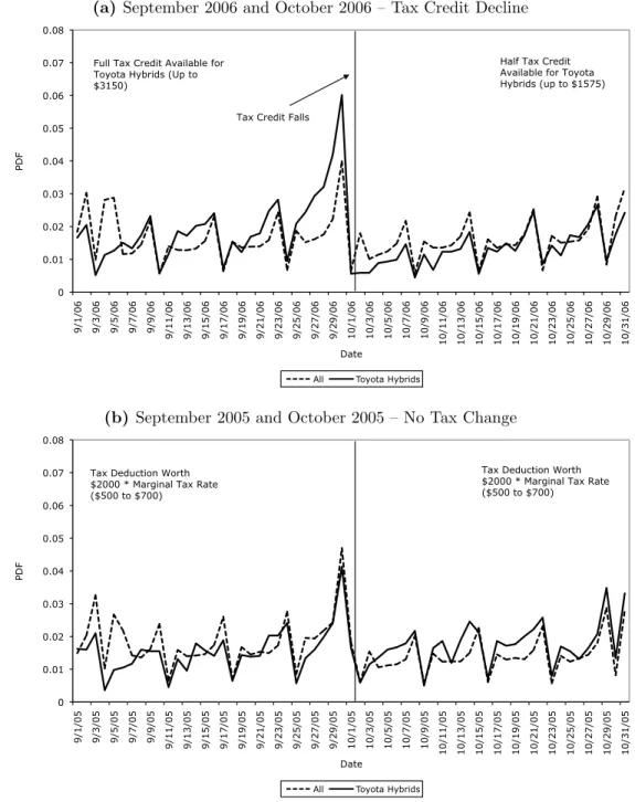
During the available sample period for the data, Toyota models experienced two addi-tional changes as the credit phased out. All credits fell by 50% of their value on October 1, 2006, and they fell again to 25% of their original value on April 1, 2007. Figures 3 and
3Data come from a nationally representative sample of transactions from an industry source. See Sallee
Figure 2: Shifting of Hybrid Transactions into Tax Preferred Time Period: December and January
(a) December 2005 and January 2006 – Tax Credit Increase
0 0.01 0.02 0.03 0.04 0.05 0.06 0.07 0.08 12/1/05 12/3/05 12/5/05 12/7/05 12/9/05 12/11/05 12/13/05 12/15/05 12/17/05 12/19/05 12/21/05 12/23/05 12/25/05 12/27/05 12/29/05 12/31/05 1/2/06 1/4/06 1/6/06 1/8/06 1/10/06 1/12/06 1/14/06 1/16/06 1/18/06 1/20/06 1/22/06 1/24/06 1/26/06 1/28/06 1/30/06 PDF Date
Figure 2: Distribution of Sales December 2005 and January 2006 (Hybrids and All Other Vehicles)
All Hybrids
Tax Credit Worth Up To $3150 Tax Deduction Worth
$2000 * Marginal Tax Rate ($500 to $700)
Tax Deduction Ends Tax Credit Begins 1/1/06
(b) December 2004 and January 2005 – No Tax Change
0 0.01 0.02 0.03 0.04 0.05 0.06 0.07 0.08 12/1/04 12/3/04 12/5/04 12/7/04 12/9/04 12/11/04 12/13/04 12/15/04 12/17/04 12/19/04 12/21/04 12/23/04 12/25/04 12/27/04 12/29/04 12/31/04 1/2/05 1/4/05 1/6/05 1/8/05 1/10/05 1/12/05 1/14/05 1/16/05 1/18/05 1/20/05 1/22/05 1/24/05 1/26/05 1/28/05 1/30/05 PDF Date
Figure 2: Distribution of Sales December 2004 and January 2005 (Hybrids and All Other Vehicles)
All Hybrids
Tax Deduction Worth $2000 * Marginal Tax Rate ($500 to $700)
Tax Deduction Worth $2000 * Marginal Tax Rate ($500 to $700)
Note: The “hybrids” series includes all hybrids, regardless of manufacturer, that were eligible for a tax credit. For all of these vehicles, the introduction of the tax credit increased the real value of the tax benefit, but the amount of this change varies across vehicles. The “all” series includes all vehicles sold in the market that did not qualify for a hybrid tax benefit.
Figure 3: Shifting of Hybrid Transactions into Tax Preferred Time Period: September and October
(a)September 2006 and October 2006 – Tax Credit Decline
0 0.01 0.02 0.03 0.04 0.05 0.06 0.07 0.08 9/1/06 9/3/06 9/5/06 9/7/06 9/9/06 9/11/06 9/13/06 9/15/06 9/17/06 9/19/06 9/21/06 9/23/06 9/25/06 9/27/06 9/29/06 10/1/06 10/3/06 10/5/06 10/7/06 10/9/06 10/11/06 10/13/06 10/15/06 10/17/06 10/19/06 10/21/06 10/23/06 10/25/06 10/27/06 10/29/06 10/31/06 PDF Date
Figure 2: Distribution of Sales September 2006 and October 2006 (Toyota Hybrids and All Other Vehicles)
All Toyota Hybrids
Half Tax Credit Available for Toyota Hybrids (up to $1575) Full Tax Credit Available for
Toyota Hybrids (Up to $3150)
Tax Credit Falls
(b) September 2005 and October 2005 – No Tax Change
0 0.01 0.02 0.03 0.04 0.05 0.06 0.07 0.08 9/1/05 9/3/05 9/5/05 9/7/05 9/9/05 9/11/05 9/13/05 9/15/05 9/17/05 9/19/05 9/21/05 9/23/05 9/25/05 9/27/05 9/29/05 10/1/05 10/3/05 10/5/05 10/7/05 10/9/05 10/11/05 10/13/05 10/15/05 10/17/05 10/19/05 10/21/05 10/23/05 10/25/05 10/27/05 10/29/05 10/31/05 PDF Date
Figure 2: Distribution of Sales September 2005 and October 2005 (Hybrids and All Other Vehicles)
All Toyota Hybrids Tax Deduction Worth
$2000 * Marginal Tax Rate ($500 to $700)
Tax Deduction Worth $2000 * Marginal Tax Rate ($500 to $700)
Note: The “Toyota hybrids” series includes only Toyota hybrids – all other manufacturers experienced no tax change in October 2006. Toyota hybrids all experienced a 50% reduction in the value of the tax credit on October 1, 2006. Hybrids made by other manufacturers, and all non-hybris, are included in the “all” series.
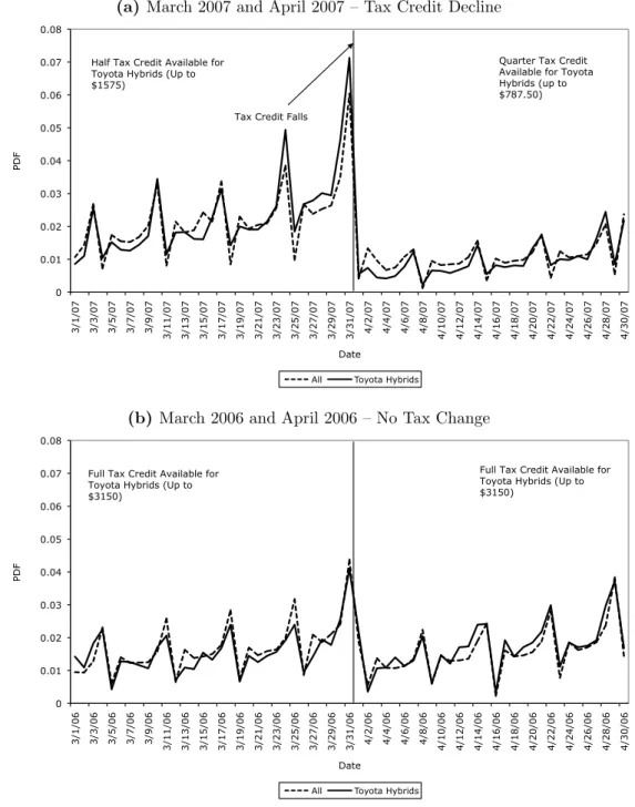
Figure 4: Shifting of Hybrid Transactions into Tax Preferred Time Period: March and April
(a)March 2007 and April 2007 – Tax Credit Decline
0 0.01 0.02 0.03 0.04 0.05 0.06 0.07 0.08 3/1/07 3/3/07 3/5/07 3/7/07 3/9/07 3/11/07 3/13/07 3/15/07 3/17/07 3/19/07 3/21/07 3/23/07 3/25/07 3/27/07 3/29/07 3/31/07 4/2/07 4/4/07 4/6/07 4/8/07 4/10/07 4/12/07 4/14/07 4/16/07 4/18/07 4/20/07 4/22/07 4/24/07 4/26/07 4/28/07 4/30/07 PDF Date
Figure 2: Distribution of Sales September 2006 and October 2006 (Toyota Hybrids and All Other Vehicles)
All Toyota Hybrids
Quarter Tax Credit Available for Toyota Hybrids (up to $787.50) Half Tax Credit Available for
Toyota Hybrids (Up to $1575)
Tax Credit Falls
(b) March 2006 and April 2006 – No Tax Change
0 0.01 0.02 0.03 0.04 0.05 0.06 0.07 0.08 3/1/06 3/3/06 3/5/06 3/7/06 3/9/06 3/11/06 3/13/06 3/15/06 3/17/06 3/19/06 3/21/06 3/23/06 3/25/06 3/27/06 3/29/06 3/31/06 4/2/06 4/4/06 4/6/06 4/8/06 4/10/06 4/12/06 4/14/06 4/16/06 4/18/06 4/20/06 4/22/06 4/24/06 4/26/06 4/28/06 4/30/06 PDF Date
Figure 2: Distribution of Sales March 2006 and April 2006 (Toyota Hybrids and All Other Vehicles)
All Toyota Hybrids
Full Tax Credit Available for Toyota Hybrids (Up to $3150)
Full Tax Credit Available for Toyota Hybrids (Up to $3150)
Note: The “Toyota hybrids” series includes only Toyota hybrids – all other manufacturers experienced no tax change in April 2007. Toyota hybrids all experienced a 50% reduction in the value of the tax credit (down to one-quarter of the original amount) on April 1, 2007. Hybrids made by other manufacturers, and all non-hybris, are included in the “all” series.
4 show the same distributional figures for those time periods. In this case, the incentive is to accelerate transactions into the earlier month. This pattern again emerges. It is absent in the bottom panels of these figures, which show the same distributions in the prior year when there were no tax changes.
This timing response is important for two reasons. First, if policy evaluators mistake such intertemporal shifting for permanent sales responses, they may overstate the effect of the policy. A simple before-after comparison of the number of vehicles sold after the tax subsidy increased would overstate the impact of the policy on the relevant externalities. Second, this intertemporal shifting is fiscally wasteful; it increases the fiscal outlay without putting extra hybrids on the road. The Canadian feebate program was introduced as a surprise and subsequently did not witness the same shifting. Where possible, revenue can be saved via the element of surprise, though it should be noted that automakers complained of being ill-prepared for the Canadian policy.
6.2
Notches cause small manipulations of fuel economy
Timing responses are a short-run phenomenon. In the medium run, fuel economy tax notches create incentives for automakers to “tweak” vehicle design in ways that have very small impacts on fuel economy but large tax implications. It takes several years to design a new automobile or to change core characteristics of a body or engine. Over the course of a few months, however, minor design decisions can be made that change fuel economy by .1 or .2 mpg – like vehicle light-weighting, the addition of aerodynamic features like spoilers or belly-pans, and tire modification to change rolling resistance. When automakers discover that a vehicle is very close to a tax notch, they may be able to modify the vehicle to improve its tax status through such means.
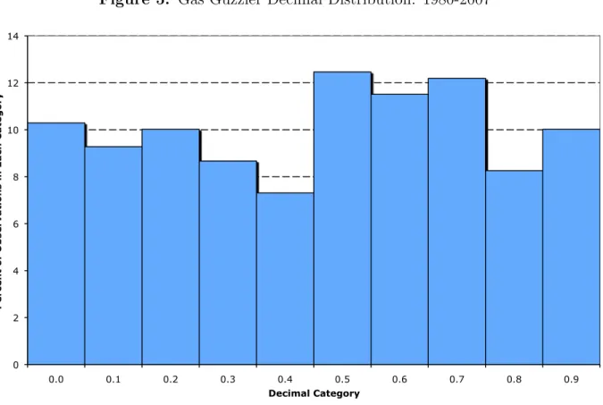
Sallee and Slemrod (2010) show that automakers do indeed respond to such incentives in the U.S. Gas Guzzler Tax, the U.S. fuel economy label rating program and the Canadian feebate program. They show that the distribution of decimal ratings of vehicles subject to
Figure 5: Gas Guzzler Decimal Distribution: 1980-2007 0 2 4 6 8 10 12 14 0.0 0.1 0.2 0.3 0.4 0.5 0.6 0.7 0.8 0.9
Percent of Observations in Each Category
Decimal Category
Gas Guzzler Decimal: All Vehicles, 1980 - 2009 (N=1,477)
Source: Sallee and Slemrod (2010). Data come from the Internal Revenue Service. Total sample size is 1,477. Tax liability falls at the .5 category. In 1980, 1981, 1983 and 1985, tax liability changed at whole integers (the .0 category) rather than at half-integers (the .5 category), so observations from those years are shifted to make the notch location consistent.
the Gas Guzzer Tax and fuel economy labels shows significant bunching on the tax preferred side. Gas Guzzler Tax liability falls at every .5 decimal – 13.5 mpg, 14.5 mpg, etc. If automakers respond to these incentives by making minor modifications to vehicles that are just below a tax notch (at 13.4 mpg, 14.4 mpg, etc.), then we would expect to find relatively few vehicles that, in the end, have a fuel economy rating ending in .3 or .4, and many with a fuel economy rating ending in .5 and .6.
Figure 5, replicated from Sallee and Slemrod (2010), shows the distribution of fuel
econ-omy rating decimals for vehicles subject to the Gas Guzzler Tax over its entire history. As
predicted, there are many more vehicles with fuel economy ratings ending in .5 or .6 mpg, which means that they are just on the tax-preferred side of a notch. This suggests that
automakers make small modifications to vehicles that happen to be just below a tax notch, but they do not apply those same changes to vehicles that happen to be further away.
The welfare implications of this behavior are negative because this medium-run tweaking corresponds to design choices that make very small improvements in fuel economy in order to generate very large changes in tax treatment. Sallee and Slemrod (2010) estimate that the net impact of these local manipulations amount to a negative welfare impact equal to three times the positive welfare impact that can be expected from a smooth, ideal Pigouvian tax. While notched tax schedules may be simpler to legislate, they create negative welfare implications from this medium-run manipulation, which would not exist in a smooth schedule.
6.3
Policies invite relabeling of vehicles as light trucks
In the medium run when engine characteristics and body style are fixed, automakers have a limited menu of options for changing fuel economy. In the long run, they can modify the engine, transmission and core body characteristics in response to policy. These long-run changes are the intended effects of the policy, but a further unintended consequence stems from the distinction between passenger cars and light trucks. Because light trucks receive more favorable treatment under CAFE and are exempt from the Gas Guzzler Tax, automakers have an incentive to relabel cars as trucks whenever possible.
The regulatory definition of a light truck is a vehicle that is a “truck derivative” (hence a truck) that has gross vehicle weight and curb weight below specific thresholds (hence light). The definition of a truck derivative is not precisely defined in the statute, but in practice vehicles built on a truck chassis that have truck characteristics (like four-wheel drive, flat beds, and a higher clearance that facilitates off-road driving) are deemed trucks.
Consequently, all minivans and SUVs are classified as light trucks, and a variety of other vehicles like Subaru station wagons, the Chrysler PT Cruiser and Chevrolet HHR also qualify. Three waves of vehicle design have achieved a transformation of the passenger car versus light truck share of the market. First, minivans supplanted station wagons and large sedans
as the modal family car starting in the late 1980s. Second, SUVs further displaced higher-end sedans in the 1990s. Third, so-called cross-overs, almost all of which qualify as light trucks, are currently rising in market share, further displacing sedans. Overall, light trucks now account for roughly half of the personal vehicle market, whereas they were a modest 10% in 1978.
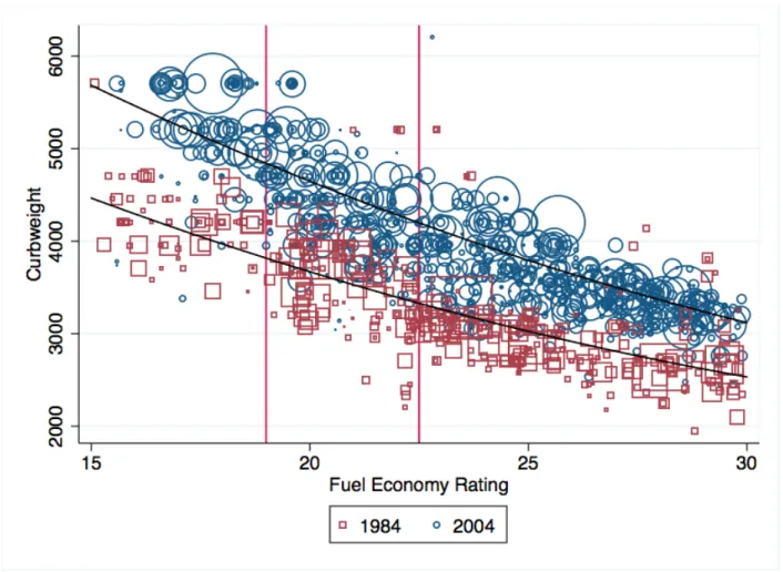
The precise nature of this transition suggests automaker attention to fuel economy tax-ation. Figure 6 shows the relationship between curb weight (a common measure of vehicle size) and fuel economy (using the Gas Guzzler Tax rating value) for passenger cars in 1984 (the earliest year with available data) and 2004. Each circle or square in the figure represents a CAFE rated vehicle configuration, and the size of the shape indicates sales volume. The solid lines are quadratic regression lines. In 1984, the Gas Guzzler Tax was still phasing-in, and vehicles were taxed only if their fuel economy was below 19. Once fully phased-in, the Gas Guzzler Tax applied a minimum $1,000 tax to all vehicles getting 22.5 mpg or below, and the figure has a vertical line to indicate this cut-off.
Figure 6 shows that fuel economy technology improved – a vehicle of the same weight in 2004 had significantly higher fuel economy than in 1984. In 1984, there are very few vehicles getting below 19 mpg, the cutoff for the Gas Guzzler Tax. This discontinuity shifts sharply to 22.5 mpg, the new tax cutoff, in 2004, by which time passenger cars getting below 22.5 mpg had all but disappeared.
Figure 7 shows the same figure, but it includesboth passenger cars and light trucks. Once
light trucks are included, there is no apparent drop-off in vehicles getting below 22.5 mpg in 2004. There does appear to be technological improvement – the schedule is shifted out – but there is no movement away from low fuel economy vehicles around the Gas Guzzler Tax. One explanation is that automakers have continued to sell heavy vehicles to consumers willing to pay for size, but they have avoided the tax by transforming these vehicles into light trucks. Figure 7 does suggest a discontinuity in the entire vehicle market at 19 mpg in 1984. This is consistent with the idea that it takes several years to make the vehicle classification
Figure 6: Curb Weight and Fuel Economy in 1984 and 2004: Passenger Cars
Source: Sallee and Slemrod (2010).
changes exhibited later.
Figure 8 presents a different way to show a similar result. This figure plots the market share of vehicles that get between 20 and 22.5 mpg for passenger cars and all vehicles (cars and trucks combined). The car series shows the near extinction of vehicles in that fuel economy category. But, the rise of light trucks that get between 20 and 22.5 mpg almost completely offsets this trend over the period.
In a simple Pigouvian framework of gasoline conservation, there is no justification for treating light trucks and passenger cars separately. If either vehicle type generates a negative social externality by consuming gasoline, the efficient response is to tax that gasoline at the Pigouvian level. The same intuition holds for taxing fuel economy. The preference given
Figure 7: Curb Weight and Fuel Economy in 1984 and 2004: Passenger Cars and Light Trucks
Source: Sallee and Slemrod (2010).
to light trucks has created a long-run design distortion that causes costly vehicle redesign and manipulation that improves tax treatment without necessarily improving (and perhaps harming) the targeted outcome – gasoline consumption.
7
Taxes do not put a consistent price on gasoline
con-servation
As described above, the ideal Pigouvian tax is efficient because it places a consistent tax on the consumption of a gallon of gasoline so that all consumers and producers face a common
Figure 8: Percentage of Vehicles Rated Between 20 and 22.5 MPG: Passenger Cars and All Vehicles 0% 5% 10% 15% 20% 25% 1975 1980 1985 1990 1995 2000 2005 2010 Pe rc en ta ge Year All Cars
Source: Author’s calculations of NHTSA data.
incentive to reduce consumption. Fuel economy taxation, however, faces several obstacles to achieving this incentive parity. To understand why, it is helpful to first describe the relationship between fuel economy and gasoline consumption.
The number of gallons of gasoline consumed by a vehicleg can be written as the number
of miles driven m divided by fuel economy written as miles-per-gallonmpg:
g = m
mpg. (2)
Because mpgis in the denominator, the relationship between gasoline consumption and fuel
on the starting level of fuel economy. This relationship can be described by the derivative of the gasoline consumption function:
∂g
∂mpg =
−m
mpg2, (3)
which shows that a onempg improvement in fuel economy has agreater impact on gasoline
consumption when fuel economy is lower. Note that this would not be true if fuel
econ-omy were written as gallons-per-mile. Much of the rest of the world rates fuel econecon-omy in liters-per-hundred-kilometers, which inverts the distance-consumption relationship and makes consumption linear in fuel economy.
Laboratory experiments suggest that consumers are confused by this nonlinearity – they tend to believe that marginal increases in mpg are more valuable for vehicles with high
mpg ratings (Larrick and Soll 2008). This difference can be quite large. For purposes
of illustration, suppose that all cars are driven 120,000 miles in their lifetime, which is the assumption used in calculating conservation in the Hybrid Vehicle Tax Credit. The number of gallons of gasoline conserved by a 1 unit increase in fuel economy is therefore
120,000/mpg−120,000/(mpg+ 1). Figure 9 shows how this conservation value varies across
the fuel economy distribution. Vehicles, like the Toyota Prius, at the extreme of the fuel economy distribution conserve less than 10% of the gasoline from a 1 unit increase in mpg that is conserved by a vehicle, like the Chevrolet Silverado, at the low end. The variation in the middle is significant as well – a 1 mpg improvement for a Volkswagen Jetta that gets 25 mpg represents about twice as many gallons of gasoline as the same improvement for a Honda Civic that gets 35 mpg. Put differently, the Prius fuel economy would need to rise by 16 mpg to match the lifetime fuel savings of a 1 mpg increase in the Silverado.
To create a common tax on gasoline consumption across relevant actors, the tax on fuel economy cannot be the same cost per unit of fuel economy when rated as miles-per-gallon. Nor can it be a linear function of the percentage improvement in fuel economy. Instead, it
Figure 9: Gasoline Conserved By One Mile Per Gallon Improvement in Fuel Economy for Vehicle Driven 120,000 Miles
0 200 400 600 800 1000 1200 10 15 20 25 30 35 40 45 50 55 60 Lif e% m e Gallons Sa ve d b y 1 m pg inc re ase
Ini%al Fuel Economy (MPG)
Chevrolet Silverado
Ford Crown Victoria Volkswagen Je?a
Honda Civic Toyota Prius
Note: Example vehicles taken from 2006 EPA fuel economy data file. Ratings are the in-use shortfall adjusted combined highway and city ratings.
must be a nonlinear function.
In practice, fuel economy taxes have done a poor job of creating this consistency for two reasons. First, because these policies all feature notches, the implicit subsidy for small improvements in fuel economy will be zero for some vehicles (because the improvement is too small to move the vehicle into the next tax tier) and large for others. Figure 10 illustrates these effects for the Gas Guzzler Tax by showing the tax reduction per gallon of gasoline conserved (assuming a lifetime of 120,000 miles) for vehicles with different starting fuel economy values assuming first a .5 mpg increase and second a .1 mpg increase. Notches create three types of inconsistencies visible in this figure.
Figure 10: Gas Guzzler Tax Change Per Gallon of Gasoline Conserved for Two Different Fuel Economy Improvements
(a)For .5 mpg increase
0 5 10 15 20 25 11.5 12.5 13.5 14.5 15.5 16.5 17.5 18.5 19.5 20.5 21.5 22.5 23.5 Ta x Ch an ge p er G al lo n of G as ol in e Co ns er ve d ($ /g )
Ini9al Fuel Economy
(b) For .1 mpg increase 0 5 10 15 20 25 11.5 12.5 13.5 14.5 15.5 16.5 17.5 18.5 19.5 20.5 21.5 22.5 23.5 Ta x Ch an ge p er G al lo n of G as ol in e Co ns er ve d ($ /g )
Ini9al Fuel Economy
Note: Gasoline conservation is calculated assuming all vehicles are driven 120,000 miles in their life.
First, since notches are all at .5 mpg in the tax, a .5 mpg fuel economy improvement for a vehicle with a fuel economy rating ending in .5 - .99 will see no tax change from implementing the improvement. The resulting tax change is therefore 0, even though gasoline is conserved, and this creates the jagged schedule shown. Second, because the tiers of the Gas Guzzler Tax are not written to exactly equate tax changes with gasoline conserved, the amount of subsidy varies across notches, most notably with the last notch at 22.5 mpg, which is worth $1,000. Third, the tax change per gallon conserved is different depending on the size of the fuel economy improvement. This can be seen by comparing parts (a) and (b) in figure 10, which shows that the tax improvement per gallon conserved is much higher for small fuel economy improvements that trigger a tax change than for larger improvements. The Pigouvian ideal would subsidize a gallon of conserved gasoline at a constant level in all situations. Notched schedules, like the Gas Guzzler Tax, create capriciously varying tax incentives. This is inefficient because automakers will install fuel economy improvements on vehicles close to notches and they will not do so on vehicles far away from notches, even though the social benefits are equivalent.
Figure 11: Gallon of Gasoline Conserved Per Dollar of Subsidy Under Hybrid Vehicle Tax Credit for Two Different Vehicle Classes
Source: Author’s calculations.
The second reason that fuel economy taxes have created inconsistent incentives is that some subsidies are based on a vehicle’s proportional improvement in fuel economy over a baseline. The Hybrid Vehicle Tax Credit has this feature. It includes both a conservation credit, which is a (notched) subsidy for gallons of gasoline conserved, and a fuel economy improvement credit, which is a (notched) subsidy based on the percentage improvement in fuel economy. To determine fuel economy improvement and gasoline conserved, the
legisla-tion uses as a benchmark the averagecity fuel economy of vehicles in the same inertia weight
class – a designation used in determining fuel economy.
Because fuel economy improvement is nonlinearly related to gasoline conserved, the credit creates a highly variable subsidy per gallon of gasoline conserved, which is illustrated in figure
11. Figure 11 first shows the amount of the subsidy as a function of the vehicle’s fuel economy improvement over the baseline. This is a notched schedule. Next, the figure plots the number of gallons conserved per dollar of subsidy as a function of fuel economy improvement for two sample vehicles – one a heavy vehicle with an inertia weight class of 5,500 pounds and the other a lighter-weight vehicle with an inertia weight class of 3,000 pounds. The notches create a “saw-toothed” per gallon subsidy, which is declining as the vehicle gains larger subsidies. Because percentage improvements in fuel economy have a larger effect on gasoline consumed at lower levels of fuel economy but the subsidy is (notched) linear, this saw-tooth is declining in fuel economy improvement.
Moreover, because vehicles with lower fuel economy save more gasoline for a given per-centage improvement in fuel economy, the heavier vehicle’s schedule lies above the lighter vehicle’s, which demonstrates that more gasoline is saved per dollar of tax credit for heavier vehicles. The position of two actual vehicles is noted. The Chevrolet Silverado Four-Wheel Drive Hybrid vehicle belongs in the 5,500 lbs weight class, and it achieves a 25% improve-ment in fuel economy over its baseline. Over 120,000 miles, this equates to 1,621 gallons of gasoline saved. The truck qualifies for a $400 subsidy, equivalent to 4.0 gallons of gasoline per dollar of subsidy. In contrast, the Toyota Prius, which is the in the 3,000 lbs weight class, is a 150% improvement over its benchmark, earning a $2,500 subsidy. The Prius conserves 2,744 gallons of gasoline – which is less than twice the Silverado’s savings, yet it gains six times the subsidy. As a result, the Prius only conserves 1.1 gallons of gasoline per dollar of government revenue expended.
The point of this exercise is to illustrate that fuel economy taxation does not create consistent incentives for the conservation of gasoline. Instead, it creates incentives for im-provement that vary significantly across vehicles based on their initial fuel economy and the size of the improvement. An efficient policy would create constant incentives, but this is difficult to do when fuel economy is used as the basis for taxation because fuel economy’s relationship to gasoline consumption is complicated.
7.1
Fuel economy ratings are imprecise
Adding to the challenge of creating efficient fuel economy taxation is the fact that the fuel economy ratings upon which the policies are based are themselves far from perfect. Fuel
economy ratings cannot accurately reflect the on-road fuel economy of individual consumers
because individual driving behavior influences fuel performance. Speed, acceleration, hard-braking, cargo load and external factors all have a significant impact on realized fuel economy. The difference between EPA’s city and highway test procedures hints at the importance of this variation. All vehicles are tested separately on a city and highway course, and, on average, the city fuel economy is 19% lower than highway fuel economy. This difference is as large as the difference between a Volkswagen Jetta and a Ford Crown Victoria. The realized fuel economy of someone who drivers a vehicle primarily in stop-and-go urban traffic is very different than the fuel economy of someone else who drives an identical vehicle primarily on uncongested highways. Fuel economy tax policy has no way of accounting for these differences – it must treat these two vehicles the same.
Even ignoring individual heterogeneity, fuel economy ratings may be inaccurate on aver-age. One reason is that actual fuel economy may erode over time as a vehicle ages. Another
reason is that average driving behavior changes, so ratings become outdated. The EPA
ini-tiated the rating system in 1978, but then adjusted all ratings in the mid-1980s to account for the fact that on-road use consistently underperformed relative to the official estimates. Highway ratings were uniformly reduced to 78% of their previous levels, and city ratings were reduced to 90% of the original values.
In 2008, the EPA determined that an overhaul of the rating system was necessary to correct further inaccuracies. Over time, average highway speeds, the distribution of city versus highway driving, and the use of energy consuming features like air conditioning have changed dramatically in the population, making the old test inaccurate. For example, the EPA’s highway test had a maximum speed of 55 miles-per-hour, a gross underestimate of today’s highway speeds. The EPA determined that it required an entirely new test procedure
based on five different tests, rather than the original two. This new battery of tests is currently being phased in and the revised ratings are being used to create new label ratings on vehicle stickers.
When these revisions have been undertaken, the updated values have been used to create the fuel economy labels that consumers see when they purchase a new vehicle, but the orig-inal, inaccurate ratings are still used for CAFE and fuel economy taxes like the Gas Guzzler Tax. Presumably, the reason for this is that changing CAFE and tax policy will create winners and losers, which necessitates a political process of compromise and compensation. To avoid this, the government chose to continue using a less accurate system. The welfare implications of this are described in Sallee (2010), who shows how to characterize the social welfare loss from using mismeasured values and describes the degree of mismeasurement in the fuel economy program. In principle, ratings could be corrected so they are accurate on average as driving changes over time, but in practice the original ratings become ossified.
Yet one more reason that fuel economy taxation is imprecise is that it cannot adjust to the gasoline content of fuel. Virtually all gasoline sold in the United States now contains between 5 and 10% ethanol, and flexible-fuel vehicles are capable of running on E85, which is 85% ethanol and 15% gasoline. If two vehicles with identical fuel economy ratings use fuel with different average ethanol shares, then these two vehicles will represent different gasoline consumption and emissions profiles, even if they are driven in identical manners. Fuel economy taxes cannot account for this.
Fuel economy tax policies do not adjust to the driving patterns of individuals, so that driving heterogeneity necessarily creates idiosyncratic variation in the tax or subsidy imposed per gallon of gasoline in a fuel economy tax. Average inaccuracies may also exist. And, fuel economy taxes cannot account for variation in the gasoline content of motor fuel. In contrast, a gasoline tax would automatically adjust for all of these things without requiring policy-makers to gather new detailed information. Put simply, it is much harder to correctly design a fuel economy tax than it is to correctly design a direct tax on fuel.
8
Other justifications for fuel economy regulation
The preceding discussion focuses on the efficiency of fuel economy taxation as a tool for reducing gasoline consumption in the presence of fully rational consumers. Some advocates of fuel economy taxation argue that consumers are not fully rational in their valuation of fuel economy and that this creates an additional efficiency benefit from taxation. Another possibility is that the goal of fuel economy taxation is not to reduce gasoline directly but rather to promote new technologies that will subsequently achieve gasoline conservation in the future, through technological spill-overs or network effects. Yet another possibility is that fuel economy tax policy has desirable redistributive properties. The implications for fuel economy tax policy of these ulterior motives are explored here.
8.1
Do equity considerations justify fuel economy taxation?
The gasoline tax, taken in isolation, is regressive in the United States – lower income house-holds spend a larger fraction of their household income on gasoline than do more wealthy households, a fact which can be shown directly by looking at expenditure data. Might fuel economy taxes be less regressive? Is this a reason to prefer them over gasoline taxes?
New car buyers are wealthier than average because lower income households tend to buy used vehicles. Within the set of new car buyers, however, the relationship between income
and fuel economy is not clear a priori. No empirical studies of the incidence of a full-scale
feebate program exist, but West (2004) compares the distributional consequences of gasoline taxes to those of a tax on vehicle size, which is functionally very similar to a fuel economy
tax. West (2004) finds that a tax on size is significantly more regressive than a gasoline tax.
In addition, the regressivity of gasoline taxes is less clear than it initially appears. Poterba (1991) shows that when households are ordered according to their total consumption instea