1 Cloud Resource Provisioning and Contract Adjustment in the Backdrop of SLA Violation
Risk Mitigation
The bulk of the work was done by a doctoral student.
Abstract: Service Level Agreements (SLA) in cloud computing, with their many constructs such as price, penalty, contract duration, and server uptime guarantee, represent notable trade-offs faced by the provider, specifically between provisioning cost control and SLA fulfillment. Here we address two components of the SLA-based contract design problem in cloud services: (1) the optimal service provisioning problem which aims to fulfill the uptime guarantee assured in the SLA and (2) the pricing problem in the context of SLA violation. An algorithm minimizing expected total cost by deriving the optimal number of backup virtual machines (VMs) for the purpose of mitigating SLA violation risk is presented. We also study specific contract adjustment measures that the provider can utilize to encourage the client to accept penalty payment deferrals in the event of SLA violation. Such measures allow the provider to possibly recover from server failures in a prior period by provisioning more resources in the next period. We also present some preliminary computational results which highlight the validity of some of our assumptions pertaining to the downtime distribution and demonstrate the robustness of our algorithm to specific parameter choices.
1. Introduction and Motivation
Cloud computing deemphasizes the need for companies to maintain significant in-house infrastructure. Server instances, also known as virtual servers/machines, with various sizes and different configurations of CPU, memory, and storage are now commonly offered by cloud service providers such as Amazon Web Services (AWS), Google and Microsoft. A client can
2 rent a set of virtual machines (VMs) to remotely access resources stored in these VM from any location via Internet without purchasing, storing and maintaining large scale and expensive physical servers locally. Therefore the cost involved in local resource management has been reduced dramatically, as well as eliminating the risk emanating from capacity under-utilization or demand non-fulfillment resulting from demand decreases or increases respectively by only paying what she actually used as a client of the cloud datacenter operator. These VMs are mapped onto physical servers within a cloud datacenter maintained by a provider. Such datacenters are known to susceptible to different types of failures ranging from frequent small scale failures (such as a few isolated individual server/switch failures) to less frequent but large-scale failures (such as a rack/pod or even an entire datacenter failure) due to hardware (including power, disk and network) failures, software bugs, human errors, hacks/sabotages, or natural disasters (see Dean 2009, Gill et al 2011). Failures at physical server level necessarily lead to the unavailability of running VMs due to loss of connectivity, etc.
A cloud service provider typically enters into a Service Level Agreement (SLA) with a client guaranteeing a pre-determined level of service, e.g., 99.9% uptime guarantee of the VMs provided for the contract duration. A penalty is incurred when the service provider violates this commitment, not to mention significant loss of goodwill and reputation. A cloud services SLA therefore typically comprises of contract constructs such as price, penalty, contract duration, uptime guarantee and the length of the service window over which the uptime guarantee is assured. These constructs all interact with each other and thus the overarching problem of determining an optimal SLA between a provider and a client becomes very complex. In this research, we address two related components of this larger contract determination problem: 1)
3 the optimal service provisioning component which aims to fulfill the uptime guarantee assured in the SLA and 2) the pricing problem as it relates to the likelihood of fulfilling this guarantee.
Significant progress is being made in the area of SLA design for cloud services, largely driven by the terrific growth in emerging cloud services, rapid increase in the number of service providers and more and more clients embracing the cloud to meet their needs. These works have focused on the establishment of SLA, the detection of SLA violations, and resource allocation to meet SLA requirement. Chhetri et al (2012) proposes a policy-based framework for the automated establishment of SLAs allowing both clients and providers the flexibility to choose amongst different pricing models, and Redl et al (2012) introduces a method to find semantically equal elements from different SLAs to enable automatic selection of optimal service offer for the client since there is no general standard for SLAs specification currently. Further, an architecture which is used to detect SLA violation by resource monitoring is presented in V.C. Emeakaroha et al (2012). This architecture allocates resources for a request from clients, monitors computing resources, and translates the low-level metrics into high-level SLAs using the specified mapping rules. Cost-minimization or profit-maximization through resource allocation in relation to SLA requirements is another major topic of interest. Goudarzi et al (2012) studies the SLA-based resource allocation problem to minimize the total energy cost of cloud computing by effective VM placement. Wu et al (2011) proposes algorithms to minimize VM cost and SLA violations in the context of SaaS (Software as a Service) by effective platform layer resource allocation strategies. Hu et al (2009) develops an algorithm to determine the allocation strategy that results in smallest number of servers required with two interactive job classes. However, to the best of our knowledge, the state-of-the-art in SLA research as represented by these papers do not consider: 1) optimal resource provisioning of backup VMs for the purpose of mitigating SLA
4 violation risk, 2) probabilistic modeling of SLA violation using downtime distributions of virtualized infrastructure, and 3) contract adjustment strategies in the event of SLA violation.
A common strategy followed by providers is to allocate a set of backup VMs to substitute the failed VMs as needed, thus reducing the probability of failing to meet the SLA-specified availability requirement level. For instance, if a client demands n VMs but is supplied additional VMs, downtime would be incurred only when at least VMs fail. Note that the client only pays for the n VMs he demanded; the backups are used by the provider to mitigate the risk of SLA violation, thereby paying a penalty. Thus, deciding on the number of backup VMs is an operational decision which is typically not disclosed to the client. If the number of backup VMs needed is determined in an ad hoc manner, the provider runs the risk of either violating the SLA (through under-provisioning) or reducing his profit (by over-provisioning). The provider thus needs to determine the number of backup VMs that minimizes his expected total costs, which comprises of the operating cost and expected penalty in case of SLA violation.
Du et al (2012) provides a set of algorithms to derive the downtime distribution of a given server configuration based on the limiting behavior of the birth-death process of VM failures and repairs, using a sample path analysis. We build on that research by designing an algorithm to efficiently determine the optimal number of backup VMs to meet an SLA by utilizing certain properties of the downtime distribution. Note that downtime distribution need not follow a well-behaved probability distribution (e.g., exponential). In fact, preliminary testing using real world server log data from a large high performance computing center reveals this difficulty of finding a good fit with most well-known distributions. We have not provided the details of this distribution fitting exercise due to space limitations. Note that even if we were to find a reasonably good fit with a particular distribution, there is no assurance that data collected
5 from a different data center would also fit that distribution. We therefore develop a computationally efficient algorithm which first derives a piece-wise linear approximation of the downtime distribution using a method developed by Wang and Chaovalitwongse (2013) and then determines the optimal number of backup VMs to satisfy the uptime guarantee in a given SLA.
Next, we study the issue of SLA violation, i.e., non-fulfillment of the uptime guarantee, particularly how price may then be used as a tool to defer the penalty payments to a client. In each service window, the client in our strategy has the option of either redeeming any penalty accrued or defer it to the next period and thereby allowing the provider to possibly make up for the service shortfall in the next period. We derive the maximum price that the provider can charge under such conditions of non-fulfillment and still motivate the client to defer the penalty payments. Extant research does not examine contract adjustment strategies in the event of SLA violation, which is a necessary study given the high rate of failures in cloud datacenters.
The rest of the paper is organized as follows. Section 2 provides the algorithm to derive the optimal number of backup VMs to service a particular client SLA. Section 3 studies contract adjustment strategies (particularly using pricing) in the event of SLA violation. Section 4 provides some preliminary computational analysis providing key managerial insights and Section 5 concludes with a discussion of our ongoing research in this area.
2. Optimal Backup Provisioning Model
Since uptime guarantees are provided on a client by client basis, we study a contract between a provider and a client. We make some simplifying assumptions for analytical tractability. We assume that the provider faces a single type of failure and a 1:1 mapping of physical to virtual servers in the datacenters. This is reasonable since datacenter providers may
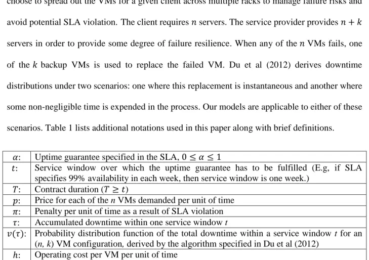
6 choose to spread out the VMs for a given client across multiple racks to manage failure risks and avoid potential SLA violation. The client requires servers. The service provider provides servers in order to provide some degree of failure resilience. When any of the VMs fails, one of the backup VMs is used to replace the failed VM. Du et al (2012) derives downtime distributions under two scenarios: one where this replacement is instantaneous and another where some non-negligible time is expended in the process. Our models are applicable to either of these scenarios. Table 1 lists additional notations used in this paper along with brief definitions.
Uptime guarantee specified in the SLA,
Service window over which the uptime guarantee has to be fulfilled (E.g, if SLA specifies 99% availability in each week, then service window is one week.)
Contract duration ( )
Price for each of the n VMs demanded per unit of time
Penalty per unit of time as a result of SLA violation
: Accumulated downtime within one service window t
: Probability distribution function of the total downtime within a service window t for an (n, k) VM configuration, derived by the algorithm specified in Du et al (2012)
Operating cost per VM per unit of time
Table 1: Notations
The provider can reduce the likelihood of SLA violation by providing more backup VMs, however this entails a higher operating cost for provisioning these backups while the client pays only for the n VMs demanded. The operating cost is therefore traded-off against the expected penalty faced by the provider. The provider therefore needs to determine the optimal number of backup VMs such that his total expected costs are minimized. The provider’s operating cost is modeled as , while the expected penalty is ∫ , as the provider does not incur a penalty if total downtime does not exceed . Further, since corresponds to the total downtime incurred within a service window, we have to subtract the
7 allowable downtime in the calculation of the expected penalty. We therefore have the following expected total cost function for a specific k:
∫ (1)
We assume that ∫ is a decreasing and convex function on . This is a valid assumption as the probability of SLA violation is likely to decline as the provider increases the number of backup VMs, ceteris paribus. In Section 4, we validate this assumption. Next, we define expected penalizable downtime as the amount of downtime accumulated during the service window in excess of the downtime allowable under the SLA specified uptime guarantee, , which is denoted by ∫ . Penalties are incurred only for the expected penalizable downtime. We can then derive the following two lemmas.
Lemma 1: The expected penalizable downtime is decreasing (1a) and convex (1b) in .
Proof of Lemma 1(a): . We get ∫ ∫ from our assumption. Since the following inequality:
∫ ∫ .
∫ ∫ , i.e. ∫
8
∫ ∫ ∫ . Since the
following inequality: ∫ ( ) ∫ ∫ .
Therefore, ∫ is a convex function in k. QED.
Lemma 2: The expected total cost is a convex function in .
Proof: From Equation (1), ,
= ∫ ( ) ∫ ∫ ∫ ( ) ∫ ∫ (∫ ( ) ∫ ∫ ) .
From Lemma 1, we get,
∫ ( ) ∫ ∫ .
(∫ ( ) ∫ ∫ ) . That is,
, or . Therefore, the expected total cost is a convex function in k. QED.
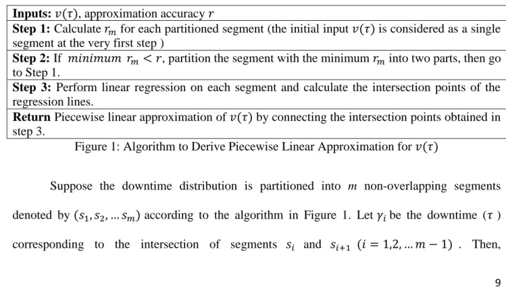
9 From Equation (1), in order to find the closed form solution to the optimal number of backup VMs, , we need Lemma 2 and a differentiable functional form of the downtime distribution. We ran extensive distribution fitting exercises on downtime distributions, specifically testing against exponential, gamma, Weibull, log normal and log logistic distributions, using the chi square goodness of fit test. None of these fit the distributions satisfactorily. We therefore use a method prescribed by Wang and Chaovalitwongse (2013) to derive a piecewise linear approximation of . Since most piecewise linear approximation algorithms rely extensively on some data-dependent threshold-based strategies, there exists a tradeoff between approximation accuracy and compression rate, which the user typically resolves via a trial and error process. Instead, we employ a two-stage top-down segmentation approach following Wang and Chaovalitwongse (2013) that first decomposes data recursively into non-overlapping intervals until all partitioned segments satisfy a data-independent threshold which is used to control approximation accuracy, and then fine-tune the linear approximation by performing least-squares linear regression. We outline this process in Figure 1.
Inputs: , approximation accuracy
Step 1: Calculate for each partitioned segment (the initial input is considered as a single segment at the very first step )
Step 2: If , partition the segment with the minimum into two parts, then go to Step 1.
Step 3: Perform linear regression on each segment and calculate the intersection points of the regression lines.
Return Piecewise linear approximation of by connecting the intersection points obtained in step 3.
Figure 1: Algorithm to Derive Piecewise Linear Approximation for
Suppose the downtime distribution is partitioned into m non-overlapping segments denoted by according to the algorithm in Figure 1. Let be the downtime ( ) corresponding to the intersection of segments and . Then,
10
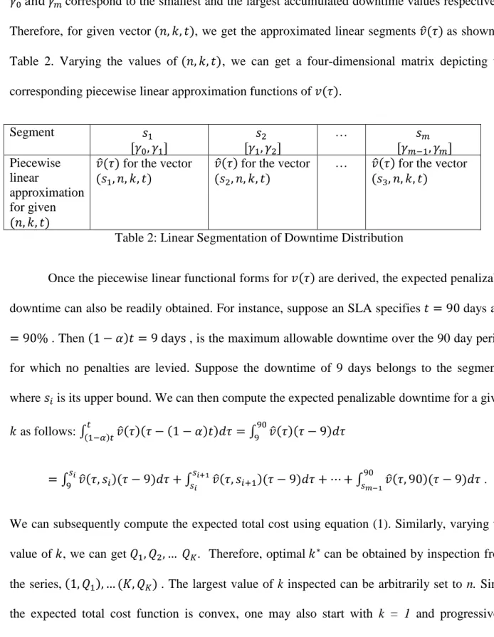
correspond to the smallest and the largest accumulated downtime values respectively. Therefore, for given vector , we get the approximated linear segments ̂ as shown in Table 2. Varying the values of , we can get a four-dimensional matrix depicting the corresponding piecewise linear approximation functions of .
Segment … Piecewise linear approximation for given
̂ for the vector
̂ for the vector
… ̂ for the vector
Table 2: Linear Segmentation of Downtime Distribution
Once the piecewise linear functional forms for are derived, the expected penalizable downtime can also be readily obtained. For instance, suppose an SLA specifies days and
. Then , is the maximum allowable downtime over the 90 day period
for which no penalties are levied. Suppose the downtime of 9 days belongs to the segment i where is its upper bound. We can then compute the expected penalizable downtime for a given
as follows: ∫ ̂ ∫ ̂
∫ ̂ ∫ ̂ ∫ ̂ .
We can subsequently compute the expected total cost using equation (1). Similarly, varying the value of , we can get . Therefore, optimal can be obtained by inspection from the series, . The largest value of k inspected can be arbitrarily set to n. Since the expected total cost function is convex, one may also start with k = 1 and progressively increase k as the expected total cost decreases and then subsequently starts to increase again. The inspection can be stopped shortly after the uptick in expected total cost is observed. In our
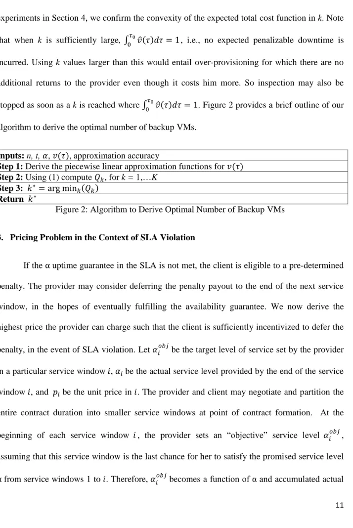
11 experiments in Section 4, we confirm the convexity of the expected total cost function in k. Note that when k is sufficiently large, ∫ ̂ , i.e., no expected penalizable downtime is incurred. Using k values larger than this would entail over-provisioning for which there are no additional returns to the provider even though it costs him more. So inspection may also be stopped as soon as a k is reached where ∫ ̂ . Figure 2 provides a brief outline of our algorithm to derive the optimal number of backup VMs.
Inputs: n, t, , , approximation accuracy
Step 1: Derive the piecewise linear approximation functions for Step 2: Using (1) compute , for k = 1,…K
Step 3: Return
Figure 2: Algorithm to Derive Optimal Number of Backup VMs
3. Pricing Problem in the Context of SLA Violation
If the uptime guarantee in the SLA is not met, the client is eligible to a pre-determined penalty. The provider may consider deferring the penalty payout to the end of the next service window, in the hopes of eventually fulfilling the availability guarantee. We now derive the highest price the provider can charge such that the client is sufficiently incentivized to defer the penalty, in the event of SLA violation. Let be the target level of service set by the provider in a particular service window , be the actual service level provided by the end of the service window , and be the unit price in . The provider and client may negotiate and partition the entire contract duration into smaller service windows at point of contract formation. At the beginning of each service window , the provider sets an “objective” service level , assuming that this service window is the last chance for her to satisfy the promised service level from service windows 1 to . Therefore, becomes a function of α and accumulated actual
12 service level . Note that at the end of each service window , the actual service level provided will beeither (surplus) or (deficit).
If , the availability surplus may be applied towards the next service window
, which would affect the set by the provider. That is, the provider may set in
service window and still attain from to . In case of a deficit ( ), the client has two choices. In the first, the client may accept the penalty payment from the provider at the end of service window i and the provider starts the next window with = α, regardless of the actual service level provided in the last window. Alternatively, if the provider sufficiently incentivizes the client with a lower price, she may defer the penalty payment till the next service window . In this case, the provider takes the deficit from into account when calculating . In this case, instead of paying a penalty at the end of service window , the provider needs to set in the service window to attain accumulated α across both service windows. Furthermore, should be less than in order to appropriately incentivize the client. Otherwise, the client would always prefer immediate penalty payments.
In this paper, we develop the foundations of this model by considering a tractable two-period problem. The client’s decision tree can then be depicted as shown in Figure 3. In this problem, the client makes her decision on whether to receive the penalty immediately or to defer it when the actual service level is less than the promised level ( ) at the end of the first service window. In order to design the incentives appropriately, the provider needs to model the client’s expected costs under each choice. The client’s expected cost comprises of the payment for n servers less expected penalty. Let ECA be the expected cost in period 2 if the client chooses to accept the penalty in period 1, which is modeled as follows.
13 Figure 3:Client’s Decision Tree for the Two-Period Problem
( ) ( ) ∫( ) ( ∫ ( ) ) ∫( ) ∫ ( ) – ∫ ( ) , where . 𝛼 𝛼𝑜𝑏𝑗 𝛼 𝛼𝑜𝑏𝑗 𝛼 𝛼𝑜𝑏𝑗 𝛼 𝛼𝑜𝑏𝑗 𝛼 𝛼𝑜𝑏𝑗 𝛼 𝛼𝑜𝑏𝑗 𝛼 𝛼𝑜𝑏𝑗 𝛼 𝛼𝑜𝑏𝑗 𝑝 𝑝 𝛼𝑜𝑏𝑗 𝛼 𝑝 𝑝 𝑝 𝛼𝑜𝑏𝑗 𝑓 𝛼 𝛼 𝛼
Pay penalty for t2
Pay penalty for t1
𝑝 𝑝 𝑝 𝛼𝑜𝑏𝑗 𝛼 𝑝 𝑝 𝑝 𝛼𝑜𝑏𝑗 𝑓 𝛼 𝛼 𝛼 𝛼
Pay penalty for t2
Pay penalty for t1 & t2 Service Window 2 Stop
The client makes her choice
Service Window 1 path 1 path 2 path 3 path 4 path 5 path 6
14 Likewise, let ECB be the expected cost in period 2 if the client chooses to defer the collection of penalties in exchange for a lower price in period 2. This cost is modeled as follows:
( ) ( ) ∫( ) ∫( ) ∫ ( ) ∫ ( ) , where , ∫ ( ) ( ) ∫ ( ) ∫ ( ) .
The client is indifferent between the two choices when . Hence, we get
∫ (∫( ) ) ∫ ∫ ∫( ) ∫ ( ) where ∫ ( ) ( ) ∫ ∫
15 4. Experimental Study
Here we present some preliminary computational results highlighting the validity of certain assumptions in our model, emphasizing some of our analytical results and adding insights pertaining to contract design and service provisioning.
4.1 Relationship Between Probability of SLA Violation and the Number of Backup VMs
We derive downtime distributions for using the sample path algorithm from Du et al (2012) which divides the service window into consecutive intervals of length of vanishing size. We ran two sets of experiments using t = 10 days and t = 20 days, with = 5 minutes. Each set specified k at 1, 2, 3 and 4. The SLA violation probability, (∫ ), drops to zero at k = 4 and beyond. At each level of k, the allowable downtime, , is set at four different levels – 5, 10, 15 and 20 mins. Figure 4 shows that the SLA violation probability decreases as the number of backup VMs increases in each set of experiments, confirming our assumption in Section 2.
(a) (b)
16 4.2 Impact of Approximation Accuracy
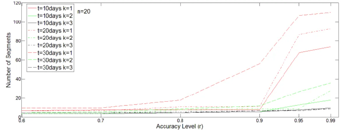
Accuracy is a specified parameter in the piecewise linear approximation algorithm which affects the number of segments into which is partitioned. As expected, in Figure 5, we can see that in general the number of segments increases along with an increase in the accuracy level. This increase in the number of segments is especially dramatic beyond the accuracy level of 0.9 and particularly so for , regardless of the length of the service window. As k increases, more segments may still be formed at higher accuracy levels but the rate of this increase steadily slows down. This makes sense as the downtime distribution is likely to have higher variance when fewer backup VMs are allocated. While the number of segments seems to be sensitive to approximation accuracy, especially at smaller k, it should be noted that the computation time is negligible with the longest being 0.065 seconds.
17 Figure 6: Sensitivity of Optimal to Varying Approximation Accuracy
Next, we explore whether a highly accurate fitting is even necessary for the piece-wise linear approximation of the downtime distribution. If does not change with a change in the accuracy level, then we may conclude that lower accuracy levels (with fewer segments) will suffice for our problem. This is especially true in light of the large number of segments when r ≥ 0.9. We generated the expected total cost curves for 24 different cases, using , n = 10 and 20; t = 10 and 20 days and r set at six levels from 0.6 to 0.99. The expected total costs across the different accuracy levels for a given (n, t, k) combination all lie within a fairly close range, which is the reason for the observing only four curves in Figure 6 in spite of actually plotting all 24 curves. The optimal k corresponds to the minimum expected total cost. As can be seen in Figure 6, regardless of the accuracy level, in each of the four sets of experiments of different (n, t) combinations, is the same. Expected penalty in the expected total cost function is calculated on the basis of the expected penalizable downtime. There is greater volatility in the range pertaining to the allowable downtime i.e., 0 to range than in the range pertaining to the penalizable downtime, i.e., to t. As a result, when greater accuracy is demanded, more segments are formed within the allowable downtime range while the segments in the penalizable downtime range remains largely unaffected. Thus, it appears that the determination of is quite
18 robust as far as approximation accuracy is concerned. Finally, we also note that the curves in Figure 6 validate the convexity result for the expected total cost function shown in Lemma 2.
(a) (b)
Figure 7: Sensitivity of Optimal to Varying Penalty and Demand 4.3 Impact of Penalty on Backup VM Provisioning
Here we vary penalty to observe its impact on the optimal number of backups VMs provisioned. As Figure 7(a) illustrates, at the lower penalty level ($5 for every 5 minutes of downtime), remains unchanged at two regardless of the number of VMs demanded and length of service window. However, when penalty is increased to $50 for every 5 minutes of downtime, increases to three when n goes from 10 to 20. At that point, the penalty is large enough where it is worthwhile for the provider to allocate one additional VM for the higher demand case. This experiment highlights the importance of setting the penalty appropriately during the negotiation process as it is shown to affect backup VM provisioning, especially at higher demand levels. 5. Conclusion and Future Research
Cloud server failures are quite common, as evidenced by some of the recent well-publicized examples involving AWS affecting the services of Netflix, Instagram, etc. Other large
19 scale failures are rarely publicized, albeit they are commonplace. In light of this, from the perspective of an Infrastructure as a Service (IaaS) provider, we propose an algorithm to determine the optimal number of backup VMs in order to minimize the expected total cost in the face of SLA violation risks. In the event of an SLA violation, we also study contract adjustment strategies using pricing as a mechanism to entice the client into deferring penalty payments. We are presently extending our experimental study in this context to explore the relationships between the second period price under SLA violation and other contract parameters such as penalty and length of service window. We are also extending our model to more comprehensively capture the multi-parameter contract determination problem as an iterative negotiation process that evolves between the provider and the client.
References
Dean, J. 2009. “Designs, Lessons and Advice from Building Large Distributed Systems”. 3rd ACMSIGOPS Intl. Workshop on Large Scale Distributed Systems and Middleware (LADIS).
P. Gill, N. Jain, and N. Nagappan. 2011. “Understanding network failures in data centers: measurement, analysis, and implications”. SIGCOMM. 350–361.
Du, A. Y., Das, S., Qiao, C., Ramesh, R. and Yang, Z. 2012. “Downtime Predictions for Virtual Servers: A Study under Two Check-pointing Scenarios”. Conference on Information Systems and Technology (CIST 2012).
Shouyi Wang, Wanpracha Art Chaovalitwongse. 2013. “An Efficient and Robust Approach for Automated Online Time Series Segmentation”. Working paper.
20 C. Redl, I. Breskovic, I. Brandic, and S. Dustdar. 2012. “Automatic SLA Matching and Provider Selection in Grid and Cloud Computing Markets.” ACM/IEEE 13th International Conference on Grid Computing.
M. B. Chhetri, Q. B. Vo, and R. Kowalczyk. 2012. “Policy-Based Automation of SLA Establishment for Cloud Computing Services.” The 12th IEEE/ACM Int. Symp. on Cluster, Cloud and Grid Computing (CCGrid 2012).
V.C. Emeakaroha et al. 2012. “Towards autonomic detection of SLA violations in Cloud infrastructures.” Future Generation Computer Systems. 28. 1017–1029.
H. Goudarzi, M. Ghasemazar, and M. Pedram. 2012. “SLA-based Optimization of Power and Migration Cost in Cloud Computing.” The 12th IEEE/ACM Int. Symp. on Cluster, Cloud and Grid Computing (CCGrid 2012).
L. Wu, S. K. Garg, and R. Buyya. 2011. “SLA-Based Resource Allocation for Software as a Service Provider (SaaS) in Cloud Computing Environments.” The 11th IEEE/ACM Int. Symp. on Cluster, Cloud and Grid Computing (CCGrid 2011).
Ye H., Wong J., Iszlai G., Litoiu M. 2009. “Resource Provisioning for Cloud Computing.” Proceedings of CASCON 2009.