Clouds-in-Clouds, Clouds-in-Cells Physics for Many-Body Plasma Simulation 1

Clouds-in-Clouds, Clouds-in-Cells Physics for

Many-Body Plasma Simulation

Charles K. Birdsall2_{and Dieter Fuss}

Lawrence Radiation Laboratory, University of California, Livermore, California 94550 Received August 22, 1968

use a 9-point difference equation for Poisson’s equation (suggested by M. Greenberg) as given in Appendix A. The

A clouds-interacting-with-clouds, clouds-in-cells method (CIC) is

presented for many-body nonlinear plasma problems. Density and motion of the individual charged particles is obtained by

force are obtained by assuming that the particles have finite size, _{integrating the Newton–Lorentz equation,} are tenuous, and may pass through one another; the particles are

thus called clouds. They obey a Coulomb force (_p1/ror 1/r3_{) when}

separated and a linear force (_pr) when overlapping, allowing simple

harmonic oscillations at small separation. CIC is contrasted with _m­v

­t5q(E1v3B).

the zero-size particle and nearest-grid-point approach, ZSP–NGP. CIC appears to have substantially less unwanted noise than ZSP– NGP and should be more useful in simulating dense plasmas. Initial

runs have been encouraging. The methods may find use in other _{The electric field E is 2=f. The magnetic field B is the} many-body simulations, such as with stars, or with particles in phase

applied field, given analytically. This integration uses the

space. Q1969 Academic Press

orbit fitting scheme given by Hockney [2].

The special problem addressed here is how to convert charge positions into charge density, and then how to

ob-INTRODUCTION

tain a consistent force on the particles. A clouds-interacting-with-clouds, clouds-in-cells (CIC)

method is being used with some advantage over a

zero-2. ZERO-SIZE-PARTICLE DENSITY AND FORCE

size-particle approach, especially with regard to reducing errors in the calculation of density and force. A major

In the zero-size-particle and nearest-grid-point method application is to many-body, nonlinear effects in fusion

(ZSP–NGP), charge density is obtained by putting the plasmas, and initial results with a two-dimensional code,

charge and mass of a particle at the nearest grid point; the SQRPLA, have been encouraging [1].

force is evaluated as if the particle were at the grid point. These choices produce zero self-force, as desired. The

re-1. PROBLEM STATEMENT

sultant force law (in two dimensions) between two like The problem is to obtain the motion of ions and electrons particles approximates a 1/r Coulomb law, in staircase fash-in their own and applied fields. The electrostatic potential ion, down to separation of one cell where the force van-fis obtained from the electric charge densityrby solving ishes; the ZSP–NGP force law is shown in Fig. 1, from Poisson’s equation, Hockney [2]. The stepped law is inaccurate and the zero force region wipes out plasma oscillations for separations between ions and electrons of less than one cell even for =2_{f5 2}r

«0 long wavelengths. Hockney [5] proposes that these diffi-culties can be reduced by using a very large number of using a 48348 grid, withfobtained at the grid points. We particles in a Debye circle, ND;nfl2D@1; n is the number density of ions or electrons and lD is the Debye length,

Reprinted from Volume 3, Number 4, April 1969, pp. 494–511. _vthermal/g_{p, where}g_{pis the plasma frequency (simple} har-1

This work was performed under the auspices of the U.S. Atomic _{monic oscillation frequency for small perturbations from} Energy Commission.

equilibrium). However, with limited computer memories 2

Permanent address: Electrical Engineering and Computer Sciences

and times, the number cannot be increased indefinitely, Department, University of California, Berkeley, CA. This author was

supported in part by A.E.C. Contract AT-(11-1)-34Proj. 128). limiting ZSP–NGP to low plasma densities. 141

0021-9991/97 $25.00 Copyright1969 by Academic Press All rights of reproduction in any form reserved.

through H5 2Dx. As the cloud size is increased beyond cell size, resolution decreases because the cloud density is held constant over a distance larger than the shortest resolvable wavelength. Of course, the density could vary within a cloud, which would be resolvable only if the cloud is larger than a cell or, as H. Berk suggests, the cloud size might vary during the problem. The method centers around reducing the potential energy of the particles as we go from a laboratory system of, say, 1015 _{particles to a computer} experiment with, say, 104_{particles; the greatest} improve-ment comes with the greatest overlapping of clouds.

The potential energy is presently calculated by summing rf. The r’s are the charge densities assigned to the grid points and the f’s are the potentials at the grid points. With this method, as an isolated cloud moves through the mesh, the potential energy is not constant, but largest for the cloud at a grid point and least in between. With many charges, these variations are small, but still undesirable.

4. CIC FORCE

FIG. 1. Zero-size-particle, nearest-grid-point force between two

posi-The CIC method uses the electric force on a cloud as tive particles. Force is zero in region2Dx/2,x, Dx/2. Adapted from

that averaged over the cloud, as given by Fig. 10 of Hockney [2].

E(x, y)effective5

O

cloud aijEp.

3. CIC DENSITY

The aij are the fractional areas as before; the Epare the In the CIC method the particle coordinates (x, y) are _{fields at the grid points where the parts of the cloud are} taken to be at the center-of-mass-and-charge of charged _{assigned. For example, for that part of the cloud placed} clouds of finite extent. The clouds are tenuous and may _{at the point i11, j 11, the x-field is given by}

pass through one another. The approach was first suggested

to us by J. A. Byers; a similar interpretation was mentioned _{2(f(i12, j11)2f(i, j11))/2Dx.} by Hockney [2]. The charge density to be assigned to points

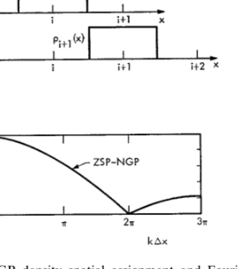
in a spatial grid is obtained by sharing the charges at several _{It is obvious that in an infinite net (walls well removed)} points. For example, using a cloud the same size as a grid _{the partial cloud produces no force on itself; A. B. Langdon} cell,Dx byDy , as shown in Fig. 2, the charge in the area _{has shown us that partial clouds, taken pairwise, produce} shaded (——_{—) is assigned to grid point (i, j ), that shaded equal and opposite forces, explosive in nature, producing} (uuuu) to (i 11, j ), that shaded ( ) to (i1 j, j1 1), and _{no net self (translational) force since the cloud has an} that shaded (////) to (i, j11). For a large number of clouds,

the charge density at (i, j ) is obtained by summing over the clouds as

r(i, j )5

O

aijrc(x, y),

whererc(x, y) is the density of the cloud at x, y and aijis the area of the cloud appearing in the cell centered at i, j divided by the area of the cell; see Appendix B.

The cloud size need not be that of a cell. As the cloud size is increased from zero, the force law begins to be smoothed out and the zero force region shrinks; the stair-casing and zero-force region are absent for cloud size equal

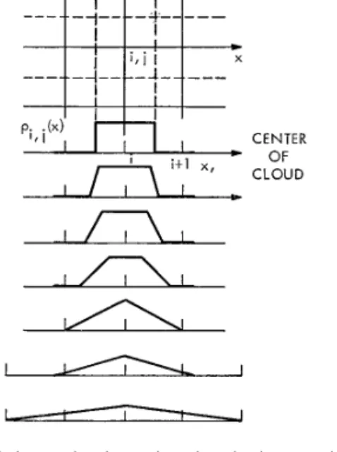
to cell size. The density appearing at i, j for a cloud moving _{FIG. 2. Cloud located in a grid, with shading showing assignment of} density to grid points for CIC method.

density is 1, otherwise, 0. In contrast, the density contours for CIC, Fig. 6, show a smooth transition from 0 to 1 over the whole region. For both models, in the region shown (i 6 1, j 6 1) the average density at point (i, j) is 1/4, assuming that the particle has uniform probability of being in this region. For CIC, the figure of 1/4 can also be inter-preted as meaning that a particle is equally shared with four points, on the average.

6. SPATIAL SPECTRA

Let us look at the spectra of charge density to see what errors are produced in the electric field because of the sampling in space.

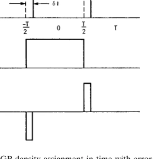
As a charge moves from cell i to cell i11, the densities assigned in ZSP–NGP to the grid points in the center of these cells vary as shown in Fig. 7a; as the particle position x passes halfway between i and i11, the density at i jumps to zero and the density at i11 to full value. Hence, point FIG. 3. Sketch of charge density assigned to (i, j ) as particle moves

past this grid point. The size of the cloud in the x direction (cloud side) i senses a thick particle which isDx on a side. For a rough

varies from 0 to 2Dx. _{measure of the apparent wavelengths produced, or spatial}

spectrum, we take the Fourier transform of this apparent density, which is simply sin(kDx/2)/kDx/2), as sketched in Fig. 7b. Note that the grid does not respond correctly implicit binding force. Thus, the CIC choices of charge

to information for kDx . f; such information is falsely and force sharing also produce no self force. The CIC force

translated to longer wavelengths (aliased). law is sketched in Fig. 4.

In CIC, the corresponding behavior is shown in Fig. 8, One peculiarity of the square clouds in the square net

the Fourier transform being the square of that above. By is that the force between two charged particles is not wholly

spreading out the charge, the spectrum is narrowed so that a central force. Because of the four-pole nature of the cloud

the amount of information that can be aliased is greatly there is a small azimuthal force which varies periodically

reduced. One may choose to use larger clouds in order to aximuthally (as does the central force). This causes two

reduce the spatial spectrum; or, if in the process of analysis overlapping clouds which are oscillating in simple

har-the Fourier spectrum of har-the density is available, har-the spec-monic (gp) motion to have an added azimuthal precession,

trum can simply be narrowed to make small clouds appear first seen by D. Wong in our 3D program, CUBic PLAsma.

larger (suggested by A. B. Langdon). If we take the infor-C. Leith points out that this will tend to produce some

mation aliased to be related to the energy, then we should angular squeezing, in our model, about a grid rotatedf/4

from the x, y grid. Remedies are to use larger clouds (more poles, more rapid decay of multipolar terms) or, more radically, a ‘‘rounder’’ grid (e.g., hexagonal); use of circular clouds with the square grid does not appear too promising, as the grid effect remains.

CIC is essentially a sharing rule for finding density and force, and proceeds just as in ZSP–NGP once the sharing is found.

5. DENSITY CONTOURS

The step from ZSP–NGP to CIC goes in the direction of particle to fluid mechanics. The ZSP–NGP density

as-FIG. 4. Force between a fixed positive charged cloud at a grid point signment is that the particle is either in or out of a given

and a negative cloud with the same y coordinate. The force approximates region. A way of illustrating this is by a contour plot of

by straight line sections the Coulomb 1/r force down to small separation density as a particle with coordinates x, y moves in the

where the law becomes linear; the clouds have simple harmonic plasma region i 6 1, j 6 1, shown in Fig. 5. If the ZSP–NGP _{oscillation for small separation. For other cloud locations in the grid, the}

details differ slightly. particle is within half a cell from the point i, j then the

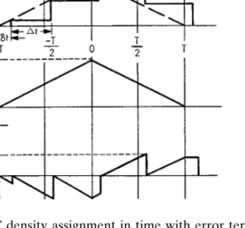
electric field; from E, the velocity v is advanced, and from the new value of v, the particles are advanced, each of the two steps being time-centered. Thus, given the position, the charge density is assumed constant forDt about time t. For ZSP–NGP, the magnitude of charge will be too small by q fordt and then T later, too large by q for dt. The range ofdt is 0,dt, Dt and the average value would appear to be d > Dt/2. One viewpoint is to say that the measured value of ri(t) is the sum of the ‘‘true’’ value (DtR0) plus an error term. For ZSP–NGP, the magnitude of the error term is q and its frequency spectrum will be quite broad, extending well beyond the time resolution available. This extension is a measure of information lost or noise added to the computation.

For CIC, a similar diagram can be made (Fig. 11). The peak error is less and the frequency spectrum of the error FIG. 5. ZSP–NGP density at (i, j ) for a particle at x, y ; (i 21)

is narrower, as the error is nearly periodic with periodDt;

Dx,x,(i11)Dx, ( j21)Dy,y,( j11)Dy.

hence there is less lost information or noise. One other point is that the peak value of the charge for CIC (b) will in general be less than that for ZSP–NGP (a), (the whole look at the square of the spectrum, in Fig. 8b, the solid charge) because the cloud on the average is shared with curve is r2

i(k) for ZSP–NGP and the dashed curve is four grid points. Hence, using r2

i(k) for CIC. If we let the information aliased be propor-tional to the area under each curve for kDx . f, then

c>bDt/2

T and b>a/4 ZSP–NGP has an area almost an order of magnitude

greater than CIC in this region.

we estimate

7. TIMING ERRORS

The errors in time may be thought to occur because the

c>

S

D

position because of the discrete sampling in time. These errors are aggravated by the size of the particle (as

con-which is a decrease in the direct error of at least an order of trasted with a smooth fluid). This effect is shown in Fig. 9

magnitude, possibly much more in the mean square error. for ZSP–NGP. With an average velocity v, the average

time used in crossing a cell of side h is called T (vT5 h), the transit time. As time advances in steps Dt, a charge may depart late bydt from one cell, hence arriving late by the same amount in the next cell, dt , Dt. If there are many particles in a cell on the average, there will be about as many arriving late as there are leaving late so that these errors will tend to cancel and produce the correct value of total charge in a given cell. The corresponding error in the vector direction of E, an error which occurs in two and three dimensions, may not be compensated this way. Unfortunately, we may not always have many particles per cell; indeed, we are more likely to average less than ten, with incomplete compensation between entering and leav-ing particles. For purposes of estimatleav-ing the size of the error, we will use only one particle.

The early–late arrival depends on the integration scheme for the equation of motion. We use the method

as given by Hockney [2], with time steps shown in Fig. 10. _{FIG. 6. CIC density contours at (i, j ) for a cloud at x, y ; (i21)} Dx,x,(i11)Dx, ( j21)Dy,y,( j11)Dy. Cloud5cell size. The charge positions give the charge densities and the

lD. Thus, even for a laboratory plasma we might write something like dn2 n2 5R 2

S

D

R2_{is the dynamical fluctuation (or shot noise) reduction} factor, generally expected to be less than unity and depen-dent on frequency, wavelength, and the volume in ques-tion, i.e., R2_5R2_{(g, k, n/N}

D). From the physics of labora-tory plasmas, one should be able to obtain the g, k dependence of R2_{; such answers may be quite complex} and obtained after considerable effort, as exemplified by similar calculations of diode noise [4]. Answers for simula-tion noise may be expected to be somewhat more difficult to extract. Hockney [2, 5] has offered some values which FIG. 7. ZSP–NGP density spatial assignment and Fourier spatial

may be applicable to ZSP–NGP but which may over-spectrum.

estimate the noise in CIC.

Some answers are available. A 1/n dependence has been observed by Barnes and Dunn [3] for shot noise using a one-dimensional electron model, aboutlDin length, with

8. SHOT NOISE, FLUCTUATIONS _{zero-size particles; from their work we find that R}2 _>

331024is implied, showing considerable interaction. The A classical approach can be used to estimate a collision _{arguments given earlier imply that short-wavelength,} high-rate or diffusion due to computational discreteness in time _{frequency fluctuations should be reduced as H is increased} and space. Let us again make rough estimates. For a gas _{from zero; the reduction in fluctuations, kE}2_{(k)l, at large} of independent and noninteracting particles, the dispersion _{k has recently been shown in theory and experiment by} about the mean value of the number in some volume is _{Dawson, Hsi, and Shanny [6] for Gaussian density slabs} and by McKee [7] for uniform density slabs. The total fluctuation level is also reduced by the use of clouds, with dn2

n2 5 1

n. appreciable reduction coming as the cloud is made larger than a Debye volume, i.e., H.lD. For such large clouds, the shielding length changes from lD to H, as originally If we choose the volume in question to be the least volume

suggested to us by J. M. Dawson and shown explicitly discernible, roughly one cell, then n will generally be on

recently by H. Okuda for a special cloud [7]. the order of 1 to 10 and the dispersion will be large indeed.

H. Berk suggests that the volume in question should have sides on the order of (1/k), where k is the largest wave-number of interest.

A special volume for plasmas is that bounded bylDon a side. For smaller volumes there can be appreciable charge separation with correspondingly large electric fields; for larger volumes, the charge separation and E fields will be smaller. Hence, one might expect the dispersion to be about 1/n for volumes up to n5NDbut to be much smaller than 1/n (or 1/ND) for larger volumes.

If we take the dispersion to be the fluctuations in charge density due to discreteness and let these fluctuations pro-duce a fictitious electric field, E2

f, then we obtain an effec-tive collision frequency which is proportional to E2

f p

dn2_{. This collision frequency would overestimate the effect} of fluctuations because the particles interact dynamically in such a way as to smooth out fluctuations rather

com-FIG. 8. CIC density spatial assignment and spatial spectrum. pletely at low frequencies and at distances greater than

of the grid transit time, the mass ratio was mi/me 5 16. Low-density runs such as these provide little test in trying to distinguish among various methods. These runs were made on the Univac Larc essentially in Fortran II.

In order to compare CIC with ZSP–NGP, computer runs were made on a medium-density warm plasma with identical initial conditions. The plasma had (gp/gc)2i>14, was cylindrical in shape bounded by zero potential walls, in a uniform magnetic field, with equal numbers of ions and electrons, mass ratio mi/me5 16, with equal kinetic energies for electrons and ions; no particles were lost to the walls. The first pair of runs used 250 electrons with ND > 3; the second pair used 5000 electrons (with the charge per cloud decreased in order to keep the plasma frequency constant) with ND>60. The results for the 500

FIG. 9. ZSP–NGP density assignment in time with error term.

charges are shown in Fig. 12 in the form of energy (total, kinetic, potential) and potential (on two probes in the plasma) versus time. Energy grows in both runs (about 500 times steps) although more slowly for CIC. The fluctu-For cold plasmas, lD5 0, ND 5 0, the physical model

ations observed in ZSP–NGP do not appear in CIC and has no randomness and, hence, no dispersion. In order to

are considered spurious. Results for 10,000 charges are observe plasma oscillations, we gave the electron clouds a

shown in Fig. 13. ZSP–NGP energy increases more slowly small velocity modulation at long wavelength and held the

(about the same as CIC for 20 times fewer particles). These ion clouds fixed, in two dimensions, H5h. With the

veloc-runs were made on a CDC 6600 using Fortran 400. One ity amplitude about one-sixth that needed for the first cloud

CIC time step was about twice as long as that for ZSP– crossing, we observed almost perfect exchange between

NGP. As most of a step was used in moving the particles, potential and kinetic energy for several cycles; at smaller

this timing would indicate that ZSP–NGP could use about velocity, the exchange was imperfect by a few percent.

twice as many particles in the same time. R. Hockney (by This defect is partially due to the deviation of the force

letter to us) has noted the same difference in times, also on individual clouds from the correct force which is

depen-using Fortran, on a gravitational problem (where, inciden-dent on the way the clouds are placed in the grid; Langdon

tally, the equivalent ND is the total number of particles). and Wong made this explanation more explicit in

one-As yet, we have little quantitative data on fluctuations dimensional theory and experiments [7], with H 5 Dx

relative to theoretical estimates. (large effect) and H510Dx (vanishingly small grid effect,

even out to kH52f).

10. OTHER APPLICATIONS 9. EXPERIENCE WITH CODE

Many-body simulation of 1/r, 1/r2_{forces with stars uses} essentially the same equations given here with a sign Our experience with the CIC method in two-dimensional

change in Poisson’s equation. Hence, star calculations of plasma problems with code SQuaRPLA has been very

good [1]. In initial trial runs we found an appreciable decrease in fluctuations of potential energy as ND was increased through unity. In subsequent runs, at low density (g2

p/g2cof ions &1), we found no direct evidence of large angle particle deflections and little or no evidence of parti-cle heating or cooling over hundreds of cyclotron and plasma periods. Perhaps the best measure of confidence has come in the constancy of total energy with no special energy conserving methods used. In spot checks during a plasma build-up run, energy was conserved to within 0.3%

for 8000 steps; in another run with 1600 clouds, hot ions and cold electrons in a nonuniform magnetic field, the energy remained constant to within60.1%for 5000 steps. Typically, the time step was 1/15 of an electron cyclotron

FIG. 10. Equation of motion integration steps. period, 1/40 of an electron plasma period, and about 1/10

type equations, collision cross sections and frequencies, dispersion relations, and so on. Such descriptions are being developed [6, 7].

APPENDIX A: POISSON SOLVER

The difference equation used for Poisson’s equation is the stencil given by Collatz [8], as follows (h5 Dx5 Dy):

8h2₌2_u

0,01h2=2u1,01h2=2u0,11h2=2u21,01h2=2u0,21

140u0,028(u1,01u0,11?1?)22(u1,11u1,211?1?)

501h 6 60

S

D

FIG. 11. CIC density assignment in time with error term.

We replaced the =2_{u by the (2r/«}

0) at that grid point. Comparing the error term with the Laplacian terms, for harmonic densities and potentials, shows that this 9-point density and force may also use the CIC approach to similar _{form produces 1 to 2 orders of magnitude less error at} advantage. Each cloud becomes a tenuous collection of _{large wavelengths relative to the widely used 5-point form.} stars. _{The method of solution, for zero potential walls bounding}

The Vlasov equation using a distribution function, f (r, _{a 48348 grid, was to Fourier analyze (r/«}

0) in x, assume

v, t )5N/d3_{x d}3_{v, could also be solved in a gridded system}

that this could also be done forf, following Hockney (and (in r, v) with clouds of N particles (fixed number) moving _{Buneman [2]), but then to solve the 47 difference equations} about phase space. Use of sharing, CIC, should also help _{for each of the 47 harmonics by Gauss elimination; the} to reduce noise due to computational discreteness.

11. CONCLUSIONS

Contrasts between zero-size-particle, nearest-grid-point and clouds-in-clouds, clouds-in-cells methods of obtaining density and force have been offered. Arguments have been put forth to show that CIC should have substantially less noise or spurious effects than ZSP–NGP, resulting in lower noise for the same ND if care is used in choosing cloud side H relative to grid side h andlD. The transition from ZSP–NGP to CIC coding requires the addition of simple sharing calculations for density and force, adding some time to each step. However, in working with denser and denser plasmas, meaning plasma diameters of more and morelD, will put demands on using the least tolerable ND, to keep the number of particles within computer capacity. Thus CIC should aid in simulating higher density plasmas. R. L. Morse (Los Alamos Scientific Laboratory) has pointed out that hydrodynamic calculations in their labora-tory use their well-known particle-in-cell method (PIC) with ‘‘area weighting,’’ analogous to our charge and force sharing, to achieve smoothing. If we claim anything at all,

it is that we are among the early users and strong advocates _{FIG. 12. Comparison runs with 500 particles, (a) for CIC and (b) for} ZSP–NGP, in a uniform magnetic field. At t50, the electron and ion of CIC for simulation of charged particles and plasmas.

kinetic energies were equal, mi/me516,tpe>6.7,tpi>26.9,tci56.28,

We are aware that what is presented here is only a

tci5100, ND>3. Run goes to T>100. The most prominent frequency

beginning, some initial persuasion and evidence that CIC

appears to be the electron hybrid with calculated periodtH54.6. The

may be useful. It will be necessary to obtain more rigorous

ZSP–NGP growth in electron kinetic energy causes the total energy theoretical physical description for clouds interacting with _{growth—which should not occur physically. There is initial potential}

energy as the ions and electrons were not overlaid at t50. clouds, with and without grids, such as Boltzmann,

Vlasov-last step is to Fourier synthesize in x to producef(x, y). In the Fourier sine analysis–synthesis, the amplitudes of like-valued sines were gathered together to reduce multi-plications; the running times appear comparable with those of more formal fast Fourier transform methods.

For a doubly periodic system with a 32 3 32 grid, we Fourier analyze the density in both x and y and obtain the Fourier amplitudes of potential directly and then synthe-size. We use a FFT routine.

In three dimensions, for zero potential walls bounding a 36 3 36 3 36 grid (>50,000 points), using a 19-point difference equation [8], the density is Fourier sine analyzed in x and y, then the difference equations are solved for the harmonics of the potential by Gauss elimination, fol-lowed by synthesis. Starting with charges on the mesh points, the time for solving for the potential is about 6 seconds, using a Fortran program on the CDC 6600. No attempt has been made to reduce this time, yet it is com-parable to that of Hockney’s two-dimensional 2563 256 (>65,000 points) highly refined machine code Poisson solver [9].

APPENDIX B: CHARGE SHARING FIG. 13. Same as Fig. 12 but for 10,000 particles and somewhat shorter

total time, ND>60. The charge per particle was reduced to maintain

the same plasma frequency; the cyclotron frequencies were also the same. The charge sharing expression in Section 3 is written

The ZSP–NGP spurious effects are much smaller, but total energy still in-out here for the rectangular cloud shown in Fig. 2, Hx 5

creases. Dx , Hy 5 Dy. The origin for x, y is taken as i, j ; x and y

must fall within the four grid points named on the figure,

accomplished in the code by determining the lower-left- CA. J. Dawson is at Princeton University, Princeton, NJ. We are also indebted to R. von Holdt (LRL), for mathematical insight in solving hand grid location (by truncation forDx5 Dy51).rcis

Poisson’s equation. the charge density of the cloud:

REFERENCES

r(i, j )5rc

(Dx2x)(Dy2y)

DxDy 1. C. K. Birdsall and D. Fuss, Bull. Am. Phys. Soc. 13, 283 (1968). 2. R. W. Hockney, Tech. Rep. SUIPR No. 53 (Stanford University,

Stan-ford, CA, May 1966); Phys. Fluids 9, 1862 (1966).

r(i11, j )5rc

x(Dy2y)

DxDy 3. C. Barnes and D. A. Dunn, in Proc. Symposium on Computer Simula-tion of Plasma and Many-Body Problems, College of William and Mary, Williamsburg, VA, Apr. 19–21, 1967 (NASA SP-153).

r(i11, j11)5rc xy

DxDy 4. C. K. Birdsall and W. B. Bridges, Electron Dynamics of Diode Regions (Academic Press, New York, 1966, Chap. 6.

5. R. W. Hockney, Tech. Rep. SUIPR No. 202 (Stanford University,

r(i, j11)5rc

(Dx2x) y

DxDy . Stanford, CA Oct. 1967); also, Phys. Fluids 11, 1381 (1968). 6. J. M. Dawson, C. G. Hsi, and R. Shanny, in Proc. Conference on

Numerical Simulation of Plasma (Los Alamos Scientific Lab., Los

ACKNOWLEDGMENTS

Alamos NM, Sept. 18–20, 1968) (LA-3990).

7. C. K. Birdsall, A. B. Langdon, C. F. McKee, H. Okuda, and D. Wong, We are indebted to many for suggestions, as identified in the text.

in Proc. Conference on Numerical Simulation of Plasma (Los Alamos M. Greenberg, A. B. Langdon, and D. Wong are at the University of

Scientific Lab., Los Alamos, NM, Sept. 18–20, 1968). California, Berkeley. We have had fruitful exchange with O. Buneman

8. L. Collatz, The Numerical Treatment of Differential Equations and R. Hockney of Stanford University through quarterly seminars and

(Springer-Verlag, New York, 1966), p. 542 (9-point), p. 546 (19-point). are especially grateful to Dr. Hockney for his critical review of this paper

and constructive criticisms. H. Berk, J. Byers, and C. Leith are at the 9. R. Hockney, in Proc. Conference on Numerical Simulation of Plasma (Los Alamos Scientific Lab., Los Alamos, NM, Sept. 18–20, 1968). Lawrence Radiation Laboratory, University of California, Livermore,