Debt and Default in the 1930s: Causes and Consequences

NBER WORKING PAPER SERIES

DEBT AND DEFAULT IN THE 193Os: CAUSES AND CONSEQUENCES

Barry Eichengreen

Richard Portes

Working Paper No. 1772

NATIONAL BUREAU OF ECONOMIC RESEARCH 1050 Massachusetts Avenue

Cambridge, MA 02138 December 1985

The research reported here is part of the NBER's research program in International Studies. Any opinions expressed are those of the

NBER Workina Paper #1772 December

1985

Debt and Default

and Consequences

ABSTRPcr

This

on sovereign debt, adapting models of debt capacity to the circumstances of the interwar years. We consider the choices available to investors in those

foreign loans which lapsed into default in the 1930s, emphasizing the distinction between creditor banks and bondholders. _{Finally, we provide the first}

estimates of the realized rate of return on foreign loans floated between the wars, based on a sample of dollar and sterling bonds issued in the 1920s.

Barry Eichengreen

Richard Portes

Departnent

of Economics

Departxrnt of

Harvard University

Birkbeck College

Caithridge, M\ 02138

7-15 Gresse Street

London W1P ]PA

Debt and Default in the 1930s: Causes and Consequences Barry Eichengreen

Richard Portes

1. Introduction

Observers familiar with the history of international

lending approach the "debt crisis" of the 1980s with a sense of deja vu. The debt—servicing difficulties experienced in recent years by many Latin American and Eastern European nations represent only the latest in a series of similar episodes stretching back over a period of _centuries. Not infrequently did the problems encountered by sovereign borrowers culminate in default, the widespread defaults of the 1930s being merely the most dramatic and generalized instance of a repeated_phenomenon. Quite often, defaulting debtors were able to re—enter the international capital market only to default again, occasioning criticism of creditors for engaging in reckless lending ascribed to myopia or excessive

competition.

The widespread defaults of the 1930s offer the most _suggestive precedent for recent difficulties. In the l930s as in the 1980s, illiquidity was not confined to any one country or region. In neither instance can the problems experienced by external debtors be attributed exclusively to domestic economic and political developments rather, they must be linked to disturbances to the

world

each instance, real interest rate shocks, commodity price fluctuations and exceptionally severe recessions in industrialized regions. The extent of the parallels has tempted many observers to see in recent developments the potential for a replay of the collapse of international capital markets witnessed in the 1930s.

Skeptics object that institutional arrangements governing international lending have changed so fundamentally that interwar experience contains few meaningful lessons for the 1980s. Perhaps the most prominent institutional innovation is the switch from bond to bank finance, a development which, by changing the provisions of loan

contracts and reducing the number of creditors party to negotiations, is said to facilitate rescheduling of debt as an alternative to outright default. The International Monetary Fund now provides illiquid

borrowers an external lender of last resort which at the same time

serves the capital market in a signaling capacity, providing information on domestic adjustment programs. Analogous to the foundation of an international lender of last resort, the establishment of domestic lenders of last resort, the spread of deposit insurance and the

implementation of macroeconomic stabilization policies are said to have diminished significantly the likelihood of a business cycle downturn on the scale of the Great Depression, thereby reducing the danger that borrowing countries will again be so severely affected by vicissitudes in the industrialized world.

In the absence of a systematic analysis of the interwar record with which recent developments might be compared, it is difficult to

determine the relevance of this historical experience to recent

comparison, this paper sets out to analyze the pattern of borrowing, the incidence of default and the returns realized by foreign lenders. Its first part describes the contours of international lending in the 1920s and 1930s. Drawing on work by Eaton and Gersovitz (1981) and other investigators of the experience of the 1970s, we use regression analysis to summarize cross—section variations in the pattern and magnitude of sovereign indebtedness. The next part of the paper considers the incidence and correlates of default, estimating variants of modern models of debt capacity to explore the extent of association between standard measures of economic structure and performance and subsequent interruptions to debt service. In the final part of the paper we

provide a long—run perspective on default and on the remedies available to creditors. The provisions of loan contracts are reviewed with an _eye toward analyzing the scope for renegotiation. We then present new

estimates of the rate of return on foreign loans floated in the 1920s, disaggregating these estimates between loans in default and loans in good standing as a way of constructing a measure of the costs of default as incurred by lenders, and comparing realized rates of return on loans

made in different years, to different countries and to different classes of borrowers.

We are conscious that this paper only skims the surface of a topic with many additional dimensions deserving exploration. Our defence is that establishing the quantitative dimensions of international borrowing and lending in the 1920s is a necessary precondition for analyzing other quantitative and qualitative aspects of the problem certain to be of interest. In the concluding section to this paper, we therefore indicate the most promising directions for research.

2. Who_Were

the

Between the

wars,

exclusive preserve of the United States and a few countries of Northwest Europe. Of the long—term foreign investments outstanding in 1938, the

vast majority were assets of the United States, United Kingdom,

Netherlands, France, Switzerland and Belgium. The U.S. and U.K. alone accounted for nearly 2/3 of the gross value of long—term foreign

investments (inclusive of foreign loans, corporate securities and direct investments but excluding war debts and reparations).1/ Hence interwar trends and fluctuations in foreign investment are largely trends and fluctuations in American and British lending.

No country had as illustrious if controversial a history of foreign lending as the United Kingdom. The traditional figures suggest that more than 55 per cent of total British investment in the period 1871— 1913 was directed overseas.2/ World War I occasioned a considerable liquidation of Britain's external assets, and in the second half of the 192Os the share of new capital issues for overseas borrowers declined from its prewar range in excess of 50 per cent to 37—44 per cent before slumping to very much lower levels in the 193Os. Nonetheless, in 1938 Britain's gross—external—asset—to—gross—national—product ratio remained an impressive 79%.3/ Of these investments, half were placed in Empire

countries and 15 per cent in each of North and South America, with the remainder split evenly between Europe and Asia—Oceania. 58% of total overseas new issues floated between 1920 and 1934 was comprised of public borrowing and 7% of railway bonds, with the remainder allocated

U,

900

-J

8000

0

700

60O

0

500

400

300

200

I00

0

Foreign

Outflow,

400

1300

1200

1100

I000

900

800

700

600

500

400

300

200

0

0

0

z

0

o

N

0

0

—

ei

in

t

o

N

N

N

N

N

N

r')

p

was disproportionately concentrated in government bonds, foreign lending in other assets.4/

Tight credit conditions in London and official restrictions on the export of capital combined to encourage foreign borrowers who had

traditionally floated new issues in Britain to turn increasingly to the United States. Except for British Dominions and colonies upon whose borrowing the Colonial Stock Act of 1900 conferred preferential

treatment or who continued to borrow in London for political as much as economic reasons, for much of the 1920s London and New York were in very real competition in the flotation of overseas loans.5/ For the United States, large—scale foreign lending was a recent development. The long— term—foreign—asset/national—income ratio of the United States was still

less than 9 per cent on the eve of World War 1.6/ In contrast to Britain, America's foreign assets doubled over the course of the war

and,

after fluctuating in the immediate postwar years, soared in the

mid—'twenties. Compared to their British counterparts, American

investors

securities.7/ In contrast to Britain, where considerations of empire dominated, the geographical distribution of American investment seems to have been influenced if not governed by considerations of proximity. Nearly 40% of total American foreign investment was in Canada, 30% in Latin America and the West Indies and 20% in Europe, with the residual scattered across Africa, Asia and Oceania.8/

Figure 1 depicts the pattern of American foreign lending in the interwar years. [Figure 1 here] In the 1920s it is dominated by the

steady increase in new lending, which was maintained in each year between 1920 and 1927 with the exception of 1923, when Prance's

occupation of the Ruhr and attendant political uncertainties increased the perceived riskiness of foreign investment. Conclusion of the Locarno Pact and successful placement of the Dawes Loan in 1924 signalled full recovery of the international capital market, which continued to expand until 1928 when its growth was stifled by the portfolio shift toward domestic assets associated with the Wall Street boom. By 1929 new foreign lending had fallen back to 1924 levels, before recovering slightly in 1930 following the collapse of the stock market. In 1931, with the further deterioration of economic conditions and the first defaults abroad, lending slumped to near—negligible

levels, with Canada the only remaining major foreign borrower. By 1932 even Canadian loans had dried up, and lending remained depressed for the duration of the 1930s.

While long—term capital continued to flow out of the U.S. on

balance until the second half of 1931, as early as the beginning of 1929 the U.S. was draining liquidity from borrowing regions; in other words, from 1929 new lending fell short of the sum of interest and amortization receipts.9/ To the extent that timing conveys information about the direction of influence, the curtailment of lending cannot be seen simply as passive response to unanticipated default.

Figure 2 indicates that U.K. foreign investment generally moved in step with American capital exports, but it also shows that U.K. lending exhibited certain distinctive characteristics. [Figure 2 here] Unlike American lending, which rose steadily throughout the 'twenties, British lending was marked by a mid—decade slump, leveling off in 1922—23 and

-_

28O

260

240

220

•U)

C

0

l8O

I60

140

120

100

80

60

40

20

0

,,

.

)

c

)

)

ri,

t)

declining through 1925 before recovering through 1927. As in the _U.S., overseas lending peaked in 1928 and fell thereafter, though not _as precipitously or to such low levels. While it is tempting to ascribe the mid—decade slump in lending to tight credit conditions associated with Britain's return to gold, government policy toward new capital issues for overseas borrowers probably played the dominant role. The fluctuations in Britain's gross capital outflow depicted in Figure 2 closely mirror the changing intensity with which informal controls on capital export were enforced.1O/

Together,

the two figures suggest that the U.K. contributed less

than the U.S. both

and to the pronounced cyclical movements in their

liquidity position. In fact, the U.K. contributed nothing at all to the former during the interwar years. While the gap between the total capital inflow and outflow of the U.S. swings from large positive numbers in the late 1920s to large negative numbers in the 1930s, British interest _and amortization receipts exceed the value of the new lending throughout the interwar years, albeit by a smaller margin in the 1920s than in the 1930s.

3. Who

In contrast to foreign lending, which remained the _{preserve of a} small number of industrialized economies, a wide _{range of countries} engaged in foreign borrowing between the wars.

According to Lewis's

(1945)

America and Asia. North American debts were almost entirely offset by foreign assets, since the U.S. was by this time a net creditor, but Canada's foreign assets of US$2 billion were dwarfed by foreign

liabilities three times that size. Whether one considers gross or net foreign liabilities, Canada rather than the countries facing highly— publicized debt—servicing difficulties was the world's most heavily indebted nation by the end of the interwar years.11/

The leading debtors of the Asia—Oceania group, Australia and India, were

like Canada members of the British Empires The foreign obligations

of both countries, owed predominantly to the United Kingdom, largely

took

After North America and Asia—Oceania, Continental Europe was the most heavily indebted region. Even excluding war debts and reparations, more than a quarter of Europe's gross foreign obligations was comprised

of Germany's external liabilities. After having attained creditor status in the decades preceding World War I, some 90% of German foreign assets had been liquidated during the war or as part of the postwar settlement Germany then received extensive capital inflows between the time of the Dawes Loan in 1924 and the imposition of exchange control in

1931. The countries of Eastern Europe were also external debtors; the bulk of their external obligations took the form of sovereign debt, although western investment in extractive industries such as Romanian oil, Polish zinc and Yugoslav copper and bauxite achieved significant levels.

Given the attention devoted to Latin American debt, it is

Interesting to note that the value of Latin America's gross external obligations was smaller than the obligations of these other continents. Concern may have been heightened by the fact that Latin American debt was heavily concentrated in certain countries. Thus, Argentina ranked behind only Canada and Australia in terms of the value of gross external debt. However, only 1/6 of this total was public debt; the rest took the form of direct foreign investment, of which British investment in Argentine railways and private enterprise comprised the majority.

Brazil, the second largest Latin American debtor, contrasts sharply with Argentina. Nearly 2/3 of Brazil's gross external debt represented the obligations of federal, state and local governments. The finance of

railway construction is indicative of the two national strategies: where Argentine railways were largely British owned and controlled, Brazilian

railways were owned by the state but financed by foreign borrowing.

4. Cross—SectIon Analysis of International_Borrowing

To summarize the pattern of international indebtedness between the wars in a fashion which facilitates comparisons with studies of recent decades, we estimate variants of the borrowing models advanced by such recent investigators as Eaton and Gersovitz (1981), Edwards (1984) and

Riedel (1983). While these authors each provide a theoretical rationale for their favored specification, we do not justify or defend their

estimating equations. The results of estimating their equations are reported here only as a way of providing a basis for comparison between the 1930s and 1970s.

With the exception of consumption and investment, reliable

estimates of which are simply unavailable, we have assembled information on the major variables used in recent empirical analyses.12/ Table 1 reports estimates of the equation proposed by Eaton and Gersovitz to explain the stock of debt held by borrowing countries. Total external central government debt is related to GDP, population, openness, a measure of export variability and the rate of growth of GDP. Eaton and Gersovitz use export variability to proxy for income variability and argue that it should be positively related to desired borrowing. They use openness to proxy for the magnitude of the penalty incurred with

retaliation against default, which they argue should be positively related to desired lending. The sign of the coefficient on income

growth is theoretically ambiguous. Eaton and Gersovitz suggest that the rate of income growth should be positively related to the demand for borrowing, since some consumption out of future income is desired now, but that it may be negatively related to the willingness to lend, since "rapidly growing countries may have less to fear from the future effects

of

a credit embargo..."13/ If borrowers are on their demand—for—debt

schedules, this variable's coefficient should therefore have a positive

sign; but if

are credit—rationed, as it

reasonable to assume was

the

Table 1

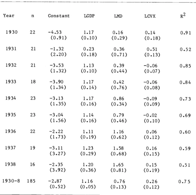
Determinants of Stock of Debt, Annual Cross Sections, 1930—8 (dependent variable is LDEBT)

Years n Constant

1930 20

1936 22

0.16 —6.15

0.48 —2.26

1938 16

Notes: Equations estimated by ordinary least squares. Standard errors in parentheses. n denotes the number of observations. Variable definitions include

LDEBT: log of total external central government debt.

SDX: _{standard deviation of exports (over years T—2, T—1, T))}

scaled (x104)

MD: _{import/GDP ratio.}

LGDP: log of GDP

LPOP: log of population.

should be interpreted cautiously for a number of reasons, not the least of which is potential simultaneity bias. The general impression

conveyed by these estimates is that the Eaton—Gersovitz model provides a less adequate account of international indebtedness in the 1930s than in the 1970s. While the results are consistent with the notion that the level of debt is positively associated with export instability and

degree of openness, the coefficients are not statistically well

determined. The only coefficient which differs from zero at standard confidence levels in every year considered is that on the log of GOP; in no case can we reject the hypothesis that this coefficient equals unity. However, there is some tendency for the coefficient of GOP to shrink in size as the 1930s progress, indicating that relatively high—income

countries had the greatest tendency to repay previously—acquired debts. By the end of the decade relatively low—GOP countries were left most heavily indebted. The predominantly negative coefficient on GOP growth can be taken as indicative of credit rationing.

The results from pooling the time—series and cross—section data are quite satisfactory and give a somewhat clearer picture, with positive coefficients on all regressors except the growth rate of GDP, all significant at the 5 per cent level except that on export instability. The coefficient on the log of GOP is so close to unity and so well determined that it seemed sensible to try debt per unit output as the left—hand variable. The consequence of deflating the stock of debt in this way is to give predominantly better determined coefficients on the remaining regressors, with no qualitative changes. The results from the pooled equation for 1930—38 are characteristic:

LDG = _—3.37

+

1.86

SDX + 1.74 ND + 0.24 LPOP —

0.001

(0.69)

=

163,

0.10,

5.02

LDG =

log

Other variables defined as in Table 1. Standard errors in parentheses.

All this uses Eaton and Gersovitz's explanatory variables for the purposes of comparative description of the data. We have not sought at this stage to use on our data the disequilibrium modelling approach which they employ. This is not because we think it inappropriate —

quite

believe, however, that it requires a tighter theoretical specification and perhaps better data than we have developed so far. Although from a quantity—rationing modeller's standpoint we might criticize the "quasi reduced form" underlying Table 1 (see Portes and Winter, 1980), it still provides interesting information about the data we do have.

Edwards (1984) has suggested that the stock demand for debt is better viewed in terms of the government's problem of selecting its optimal portfolio of assets and liabilities. Hence stocks of

international reserves and foreign debt should be simultaneously determined, and the latter will depend in general not only on the variables suggested by Eaton and Gersovitz but also on the value of reserves. We have estimated a variant of Edwards's reserve demand function, using gold reserves as our dependent variable, and obtained

Table 2

Flow of Borrowing, Cross—Sections for Three—year and Four—Year Averages 1928—1935

(dependent variable is BOR/GDP)

Notes: Equations estimated by ordinary least squares. Standard errors in parentheses. n is number of observations. Variable definitions include:

BOR/GDP: Flow of external central government borrowing as a share of GDP.

Reserves/imports *

Total

Central

*

GDP/population

Dummy variable for Latin American countries Dummy variable for Australia

denotes an average for the period.

Years n Constant RES/IMP SRV/XP DEF/GDP GDP/POP LA AUS R2 1928—30 20 —0.01 (0.02) 0.11 (0.07) —0.06 (0.09) 0.19 (0.42) 0.51 (0.61) 0.02 (0.02) 0.84 (0.06) 0.93 1928—31 21 —0.03 t ,'.\

U.UL)

U.U1)

J.UQ)

U.JI)

U.UJ)

n\

U.JJj

where

results remarkably similar to his as reported in Appendix Table Al. We then added reserves to the equation reported in Table 1, hut neither OLS nor instrumental variables estimates indicated that reserves had any impact on the level of debt.14/

Another attempt to permit balance—of--payments developments as reflected in reserves to influence the accumulation of external debt is provided by Riedel (1983), who analyzes flow supplies and demands for new borrowing rather than stocks of debt. Riedel relates the flow of borrowing to the following ratios: reserves to imports, debt service to exports, the government budget deficit to GDP, investment to national income, and income per capita. Results of estimating this equation are reported in Table 2, where we have added dummy variables for Latin America and British Empire countries (where the latter include only Australia in our sample) to flag any differences in their experiences and have dropped the investment ratio due to absence of data. The overwhelming impression is, as anticipated, one of pronounced shifts in the relationship of net lending to its determinants between 1928 and 1935. The coefficients on per capita income suggest that high income countries had the greatest tendency to borrow before 1932 and,

consistent with Table 1, to repay thereafter. Although the regional dummy variables are unstable across periods, they suggest on balance that both Australia and the Latin American countries had unusually high propensities to borrow until the total collapse of international capital markets after 1931.

Whether countries experiencing the initial effects of the Great Depression were able to use foreign funds to help finance the shock is sensitive to whether or not 1931 is included in the sample. The

positive coefficient on the reserve ratio for the period prior to 1931 suggests that even at this early date countries experiencing balance—of— payments difficulties found it relatively difficult to borrow abroad. This coefficient becomes negligible, however, when the period is

extended through 1931. Similarly, when 1931 is included in the sample, the positive coefficient on the fiscal deficit suggests that countries which chose to run deficits in response to the impact of the Great Depression initially had some ability to finance them through foreign borrowing. This evidence dissipates when 1931 is excluded from the sample. Whether the sensitivity of the results to inclusion of 1931 is due to the appearance that year of the first defaults, to the increasing inadequacy of our reserve measure given pronounced shifts between gold and foreign exchange, or to some other peculiar feature of 1931 remains to be determined.

5. Factors in Default

Part of the explanation for the incidence of default lies in special national circumstances, including particular primary commodity endowments, domestic economic policies and the uses to which borrowed funds were put. Yet in the 1930s as in the 1980s, developing countries were subjected to common external shocks which affected both the costs and benefits of interruptions to debt service. The list of common

external disturbances —

recession

will

by the resemblance of the 1930s to the 1980s should not lose sight of the greater severity of the earlier shocks.

A severe business—cycle downturn in the United States could not but exercise a powerful influence over the liquidity and solvency of

sovereign debtors. The obvious indicator of this influence is size: in 1929 the U.S. accounted for more than half of the industrial output and nearly 40% of the primary product consumption of the 15 leading

industrial economies.15/ Another indicator is the magnitude of the contraction: one need only note that the Harvard Economic Society index of the volume of manufacturing fell by 25% between October 1929 and October 1930 and that real GDP fell at twice the rate typical for the first year of a recession.16/

One of the principal channels through which these deflationary pressures were transmitted to developing regions was via primary commodity prices. In 1929, the most important agricultural goods in world trade were, in declining order of importance, cotton, wheat,

sugar, coffee, silk and rubber.17/ Countries were variously affected by their luck in the "commodity lottery,t' to use Diaz—Alejandro's (1983) term. Between 1929 and 1930 the fall in average annual dollar prices ranged from nearly 20% for wheat and tin to 30% for cotton, sugar and silk and 40% for rubber.18/ _{In many cases the fall in export prices} understates the impact on primary commodity exports. Export volumes declined with export prices as foreign demand curves shifted inwards and domestic producers moved back down their supply curves. The decline in foreign demand attributable to the depression was reinforced by

protectionist initiatives which heavily affected foreign food producers. Ironically, the measures which created special difficulty for foreign

debtors —

tariff

were

Another way of gauging the shock to indebted regions is in terms of the change in real interest rates. The fall in U.S. prices that got underway in the final quarter of 1929 raised ex post short—term real interest rates to more than 15%.19/ While the real interest rate shocks of recent years are by no means to be dismissed, they pale in comparison with the shocks experienced after 1929.

6. Cross—Section Analysis of the Incidence of Default

Existing accounts tend to portray decisions in the 1930s of whether to default on sovereign debt in one of three ways: (i) as the result of idiosyncratic national circumstances about which it is difficult to generalize, (ii) as a function of "bandwagon effects" that proved

irresistible even to basically solvent debtors once the initial defaults occurred, and (iii) as the only feasible alternative available to

developing countries given the magnitude of the shock to the world economy. Yet the incidence and extent of sovereign default varied enormously across countries. None of these approaches provides much help in understanding that incidence or that extent. This is in contrast to modern models of debt capacity, in which the incidence of rescheduling is assumed to be systematically related to a vector of

national characteristics proxying for its costs and benefits, such as

the ratio of debt to GNP and various measures of trade performance.20/ In

this section, we adapt these debt—capacity models to the

circumstances of the 1930s to examine the extent to which country—

specific

help to explain its incidence. If these variables possess explanatory power, then it will be necessary to supplement if not replace existing characterizations with an analysis of the incidence of sovereign default in the 1930s couched in terms of its differential costs and benefits across countries.

As in modern studies of rescheduling, empirical analysis is complicated by the fact that the variable of interest —

in

its dollar debt, temporarily fell into default on sinking fund early in the 1930s, before making a proposal in 1934 concerning readjustment of amortization which received the endorsement of the Foreign Bondholders Protective Council.21/ More serious was to be in default on all or a portion of interest payments. Most serious of all was repudiation, a rare event in the interwar years.22/ The best available

indicator would

appear

.

23/

Our measure of default is constructed from data covering national, state and provincial, municipal and government—guaranteed debt. The share of dollar— and sterling—denominated debt in default as to interest

or sinking fund is calculated for the period from 1934, the first year for which the newly—established Foreign Bondholders Protective Council published information on arrears, through 1938. The explanatory

variables include proxies for the burden of the debt, the degree of openness, the severity of the external shock and the stance of domestic economic policy. Given their significance in Table 2 above, dummy variables for Latin America and Australia are added to test whether political or economic factors not otherwise accounted for help to

explain the incidence of default. The external—government—debt—to— national—income ratio is used as a measure of debt—servicing

requirements —

in

openness by the ratio of exports to GDP and the severity of the external shock by the percentage deterioration in the terms of trade after 1929. It is likely that simultaneity will affect any attempt to estimate the impact of the current export share on the incidence of default, since countries which defaulted may have run policies or experienced sanctions which subsequently influenced their reliance on trade. Therefore, we use the lagged export share as a proxy for openness, employing two

alternative formulations: the 1928 export share and the export share six years prior to the year for which the dependent variable is defined. It is similarly possible that simultaneity may contaminate the coefficient on the change in the terms of trade after 1929, since countries which defaulted may then have run policies or experienced sanctions which influenced the evolution of relative prices. As an alternative to the change in the terms of trade between 1929 and the year under

consideration, we employ the change in the terms of trade between 1929 and 1931.

The next two variables are indicators of the stance of fiscal and monetary policies. To avoid problems of simultaneity, both variables are measured as percentage changes between 1929 and 1931, since

countries which defaulted thereafter subsequently had available

different policy options than countries that continued to service their external debt. The fiscal policy variable is defined as the percentage change in the central government budget deficit. Data on other levels of government, while desirable, are not available on a consistent basis. The monetary policy variable is defined as the percentage change in the ratio of gold reserves to note circulation. Almost all the countries in the sample remained on the gold standard into 1931; in the long run, therefore, their money supplies were endogenously determined. In the short run, however, governments could attempt to influence money supply and any domestic economic conditions it affected through domestic credit creation which would have as its eventual consequence a loss of

international reserves. Therefore, the greater the rise in the ratio of reserves to money supply, the more restrictive was monetary policy. While it would be desirable to include other foreign assets in addition

to gold and to use a broader measure of money supply than notes and coin in circulation, adequate data are not available for the range of

countries included here.

Two—limit probit analysis is used to analyze the incidence and extent of default in light of the fact that the observed dependent variable is obtained as zero for countries which did not default) as unity for countries in default on all their obligations, and as a range of intermediate values for countries partially in default.24/

3.25/ The

These results seem quite inconsistent with the notion that all developing countries experiencing the Great Depression had no

alternative but simply to opt for default. Rather, they suggest that the magnitude of the debt burden and severity of the external shock influenced the extent to which countries fell into arrears. At the same time, they are inconsistent with the view that non—economic factors, such as political ties to the principal creditor countries, provide the entire explanation for the incidence of default. This is not to say that the regional dummy variables can be dismissed. That for Australia has a negative sign which differs significantly from zero at any

reasonable confidence level, indicating that the extent of default was significantly less than predicted by the economic variables included in the equation, a result tempting to interpret in terms of Australia's political and cultural ties to the United Kingdom. In contrast, the incidence of default among Latin American countries is sufficiently well predicted by the economic variables in the equation that the coefficient on the Latin American dummy retains no residual explanatory power.

Table 3

Two—Limit Probit Regressions of Covariates of Default: Pooled Time—Series Cross—Section Results, 1934—1938

(dependent variable is percentage of dollar and sterling debt in default as to interest and/or amortization)

Variable (j) (ii) (iii) (iv)

Constant 0.519 0.521 0.003 0.026 (0.054) (0.047) (0.190) (0.136) Debt/income ratio 0.328 0.345 0.659 0.931 (0.164) (0.182) (0.298) (0.258) Percent deterioration, 0.223 0.567 terms of trade, 1929—31 (0.083) (0.266) Percent deterioration, 0.271 0.822 terms of trade, 1929— (0.089) (0.260) current year

Lagged export/GDP ratio 0.062 —0.326

(0.044) (0.480) 1928 export/GDP ratio 0.071 0.159 (0.207) (0.770) Percent increase in 0.005 0.005 0.005 0.004 budget deficit, 1929—31 (0.002) (0.003) (0.005) (0.003) Percent increase in 0.169 0.185 0.305 0.386 reserve ratio, 1929—31 (0.049) (0.047) (0.195) (0.186) Latin America —0.001 —0.006 (0.033) (0.052) Australia —1.253 —1.289 (0.251) (0.223) Log—likelihood —139.67 —143.06 —84.23 —81.23

Notes: Coefficient estimates are accompanied by standard errors in parentheses. Number of observations = 95. Variable definitions

include:

Debt/income ratio: total external central government debt/GDP.

Percent increase in budget deficit: central government deficit only. Percent increase in reserve ratio ratio of gold reserves to notes and coin in circulation.

The coefficient on the change in the budget deficit is positive and differs significantly from zero at the 90 per cent confidence level or better when the dummy variables for region are included. In other words, governments which ran austere budgetary policies in response to

the Great Depression were best able to avoid debt—servicing

difficulties. Those which engaged in what were by the standards of 1929—31 relatively heterodox fiscal policies had the greatest tendency to default. The obvious interpretation of this result is in terms of the absorption approach to the balance of payments —

that,

The coefficient on the monetary policy variable indicates that countries experiencing relatively large increases in the ratio of gold reserves to currency circulation had the greatest tendency to default. This result is inconsistent with the notion that countries engaging in expansionary monetary policies were driven to default by any balance of payments difficulties that resulted. Similar results have been found when estimating debt capacity models for the 1970s and interpreted to indicate that sovereign debtors anticipating eventual default hoarded reserves to finance subsequent import purchases whose expense could no longer be defrayed by additional foreign borrowing.

An alternative explanation for this result would appear to be the inadequacy of gold as a proxy for international reserves and of note circulation as a proxy for money supply. Consider for example the first of these problems. Countries in our sample held gold and convertible foreign exchange in various proportions. The use of gold reserves as a

proxy for the total would not be a problem if those proportions remained constant. However, Nurkse (1944, p.41) notes that the share of foreign

exchange in the gold and exchange reserves of 18 debtor countries for which he has information fell from 33 to 15 per cent between 1929 and

1931. Yet certain countries swam against this tide; Australia, for example, liquidated a major share of its gold reserves and replaced them with foreign exchange. Hence eliminating the dummy variable for

Australia, as in columns (iii) and (iv) of Table 3, alters the

coefficient on the monetary variable, which no longer differs uniformly from zero at the 95 per cent confidence level.26/

The mystery of the monetary variable should not be permitted to detract from the other conclusions. Overall, the results suggest that basic economic intuition and simple economic variables go a long way toward explaining the incidence and extent of sovereign default in the 1930s.

7. The Scope for Renegotiation

To understand the scope for renegotiation, it is necessary to consider the mechanics of foreign borrowing. Procedures in London and New York were quite similar. The first step for a sovereign borrower wishing to obtain funds on the London market was to issue a prospectus. Typically, the terms of the offer and solvency of the debtor had already been examined by a reputable issuing house, which endorsed the loan by attaching its name to the prospectus.27/ In New York, specialized

marketing houses played an analogous role. The revenues accruing to the managing houses took the form of the spread between the bonds' purchase

price (the price received by the foreign borrower) and the sales price (the price paid by the ultimate bondholder).

Flotation might be undertaken by a syndicate of issuing houses and banks. Since different institutions might have a comparative advantage either in negotiating an acceptable loan contract with the borrower or in marketing the bonds, it was not uncommon for one syndicate to resell a loan to another before making the bonds available to the public. Short—term advances were often extended to the foreign borrower in anticipation of successful placement of the loan. To market the securities, issuing houses based primarily in New York and Chicago

employed itinerant bond salesmen and established branch offices across the United States and Canada. Some New York banks established special security affiliates which could directly serve in this capacity without violating American branch banking laws. If at first observers hailed the verve with which these travelling salesmen trumpeted the virtues of foreign bonds, after the first defaults they accused these same

promoters of a variety of excesses.28/ The facility with which these securities were marketed is evidenced by the extent of sales to persons of relatively moderate means. Although the available statistics are incomplete, they suggest that in the 1920s the mean value of lots of foreign bonds was less than $5000. Since this figure is inflated by a small number of very large purchases, the typical lot would appear smaller still had we an estimate of the median. For example, the face value of the average holding of Chilean bonds in the 1930s appears to have been no more than $800 when the 4% of largest holdings is

eliminated.29/ The small size of holdings and large number of

in the event of default and negotiation.

There was little scope for litigation as an avenue for obtaining satisfaction from defaulting debtors. American and British courts had no jurisdiction over foreign sovereigns, who could be sued in their own courts only with their consent.30/ One way in which lenders attempted to protect themselves was by writing into loan contracts provisions which earmarked certain revenues for debt service. Unfortunately, nothing prevented a foreign government from also breaching these provisions if it fell into default on interest or amortization. Bondholders therefore tried to enlist the aid of their governments. Government involvement could range from informal negotiations through diplomatic representations and economic sanctions to armed force. The U.S. State Department maintained a policy of official noninterposition in negotiations between American bondholders and foreign governments, although diplomats and officials did not hesitate to express their interest in a settlement. The British, in contrast, permitted the bondholders to delegate a British minister to the foreign country, or his consul—general, as their local agent, a practice certain to raise questions

in the debtor's mind about the capacity in which the minister

was negotiating.31/ The use of armed force, however nostalgically

viewed

This left economic sanctions. The threat of sanctions in response to Germany's 1933—34 default illustrates the use of this instrument. In the summer of 1933 the German government declared a moratorium on the overseas transfer of interest payments.33/ Negotiations between the

head of the Reichsbank and foreign creditors ensued, yielding a compromise under which Germany agreed to meet a portion of its obligations. The Dutch and Swiss rejected the pact, however, and threatened to impose sanctions. The credibility of their threat was

enhanced by the fact that both countries ran trade deficits against Germany, implying that the costs of German retaliation were likely to exceed the benefits. The Germans settled separately with both

countries, with Dutch and Swiss nationals ultimately receiving full interest on their Dawes and Young plan bonds and cash payments of 3 1/2 to 4 1/2 per cent on most other German bonds.

Similar threats were then issued by and agreements reached with Sweden, France and Belgium. The mere opening of debate over sanctions in the British Parliament was sufficient to prod Germany into action. Before the measure could be passed into law, a German delegation arrived in London, and within a month an agreement was reached providing for full interest payments to British nationals on Dawes and Young plan bonds.34/ In contrast, the nationals of countries whose governments maintained their policy of official noninterposition received less favorable treatment. The U.S. State Department protested such

discrimination against American bondholders, but to little effect.35/ Bond finance and the associated free—rider problem are blamed for the difficulty of negotiating settlements when debt—servicing

difficulties arose. Under bank finance, illiquid debtors can turn to their creditors, who are relatively few in number, for bridging loans, while insolvent debtors can negotiate a mutually—acceptable sharing of losses. Under bond finance, creditors were allegedly too many and bond covenants too inflexible for illiquidity to result in anything but

default or for insolvent debtors and their creditors to achieve a

mutually—acceptable sharing of losses. In fact, there existed a number of mechanisms for internalizing the externalities that gave rise to free

riding.

The major difference between the interwar and postwar periods

lies not in the prevalence of negotiations designed to achieve an

equitable

default was a necessary prerequisite for getting negotiations

started .36/

The fact that bond issues were floated by issuing houses and banks meant that there existed agents sufficiently few in number and large in size to have in principle provided bridging loans. Such short—term loans and advances had been common in the 1920s (see de Cecco, 1984). Moreover, it was in the banks' interest to tide over illiquid debtors, since they suffered embarrassment from default on bonds with whose issue they had been associated. It is troubling, therefore, that little such lending occurred after 1929. It could be that the debt crisis was quickly recognized as a problem of insolvency rather than illiquidity, and that money center banks rationally refused to throw good money after bad. This hypothesis imputes considerable foresight to the lending institutions. Moreover, it overlooks the possibility that their very unwillingness to provide short—term credit may have been directly

responsible for transforming what remained a problem of illiquidity into one of insolvency. The banks' unwillingness to provide short—term loans preceded by a year the onset of default. For example, in 1930 Bolivian officials confronted with debt—servicing difficulties visited New York to "treat with" American banks. Negotiations to obtain short—term loans

were unavailing, and in 1931 Bolivia became the first Latin American debtor to default, setting off a chain reaction.37/ The alternative hypothesis is that, with only the goodwill of their customers rather

than their own assets at stake, financial institutions had little

incentive to bear the risk that what might appear to be illiquidity was really insolvency. If so, then a major difference between bank and bond finance is that under the latter, default was a necessary precondition to the successful restructuring of a loan. It does not follow, however, that under bond finance there was little scope for serious negotiation.

If default ensued, a readjustment program might be negotiated by the issuing house or by a committee it organized. Issuing houses characterized themselves as "moral trustees" obliged to protect the bondholders' interests.38/ Bondholders recognized, however, that the issuing house was likely to be torn between the interests of two sets of customers: bondholders and foreign borrowers. Moreover, the indebted government was the issuing house's single largest customer, with whom the lender was likely to have established a valued long—term

relationship. Given the potential for conflict of interest, most readjustments were therefore negotiated not by issuing houses but by independent committees. The legal status of these committees varied: some obtained the physical deposit of bonds which they were authorized to use at their discretion; others took a proxy or power of attorney from bondholders who retained possession of their certificates; and still others received no legal authorization from bondholders, who they could claim to represent only informally.

The British Corporation of Foreign Bondholders (known less formally as the British Council and less favorably as the "conscience of the

loanmongers") was the oldest such organization, having been founded in 1868.39/ With six of its 21 members appointed by the British Bankers' Association, six by the London Chamber of Commerce and nine by the Council as a whole, it could claim to represent the interests of both the City of London and the bondholding community. Until the end of 1933 there existed no comparable organization in the United States.40/

American practice was to form ad hoc committees in response to

individual defaults. The shortcomings of the method were notorious. Administrative expenses were inflated by the inability to exploit the scale economies offered by simultaneous negotiations with various

debtors. Ad hoc committees could not bring the same pressure to bear as so august an institution as the British Council. Moreover, rivalry among competing committees undermined the credibility of each. Multiple committees might be formed for various reasons, including competition for profits, since the organizers typically received a commission paid Out of debt service charges upon the conclusion of a settlement. More often, rival committees were formed when issuing houses established one and disenchanted bondholders another. The two then competed for

support, employing newspaper publicity and agents who were paid on a commission basis to secure the deposit or registration of bonds. Not only did this encourage committees and their agents to make extravagant promises, but a debtor government was faced with the problem of

determining which committee best represented its creditors. In 1933 the Foreign Bondholders Protective Council was finally established in the U.S. on a nonprofit basis. It proved a popular vehicle for subsequent readjustment negotiations, although its critics continued to suggest that it was unduly influenced by the banks.

Readjustment plans were signalled by the publication of a decree or simply an annoucement that bond covenants were henceforth modified. If the plan was a result of successful negotiations, its acceptance would be recommended by the bondholders' committee involved. A new coupon was specified and the principal might be adjusted. A new date by which the loan would be called was specified. Bondholders indicated their

acceptance of the arrangement by cashing a coupon and, when requested, by exchanging an old certificate for a new one. If acceptance of the offer was recommended by a prominent agency such as the Foreign

Bondholders Protective Council, few options remained for dissident bondholders. In theory, they could withhold their coupons and form another committee to negotiate a better settlement. In practice, foreign governments had little further interest in negotiations once their good standing had been restored by the seal of approval of the Foreign Bondholders Protective Council. Only the possibility of widespread dissatisfaction with the terms negotiated by the councils provided a check on the process.

How the bondholders fared under these arrangements is an empirical question, to which we now turn.

8. The Impact of Default and Bondholders'

Ability to

Little is known about the realized rate of return on foreign bonds purchased during the 1920s. Madden et al. (1937) estimated the current rate of return on foreign dollar bonds (excluding Canadian issues) on an accrual basis; as shown in Table 4, they took interest as it accrued

Table 4

Previous Estimates of the Rate of Return on Overseas Loans (rate of return is measured in percentage points)

Year _{Foreign Dollar Bonds Sterling Bonds in Latin America}

1920 7.67 1921 7.78 1922 7.58 1923 _{7.03 3.8} 1924 7.30 _3.9 1925 7.28 4.1 1926 7.24 _4.5 1927 7.07 _4.2 1928 7.25 _4.4 1929 _{7.03 4.5} 1930 6.90 4.3 1931 5.81 _3.2 1932 4.47 _2.0 1933 3.67 1.7 1934 6.17 1.6 1935 _{3.54 1.8} 1936 _1.9 1937 _2.2 1938 _1.7 1939 _1.6

Notes: Rate of return on foreign dollar bonds (exclusive of Canadian issues) is from Madden et al. (1937), p.154. This is interest paid in cash as a percentage of the amount invested adjusted for principal repaid in cash. Rate of return on Latin American securities quoted on the London Stock Exchange at the end of each year is from the South American Journal (January 20, 1940), p. 44. This is dividends, interest, arrears of interest and bonus as a percentage of the book value of investment.

of bonds valued at the original purchase price.41/ The figures reveal that over the decade of the 1920s the current rate of return on dollar bonds fluctuated in the range of 7—8 per cent. The highest rates of return occurred at the beginning of the decade; then between 1923 and 1929 the rate of return exhibited no obvious trend. With the onset of the Depression, that rate declined to 6.90 per cent in 1930, and in 1931 the first defaults combined with the repurchase of bonds for

cancellation at prices below par reduced the yield further. Additional defaults continued to depress the yield until 1934, when the redemption of Netherlands East Indies, Swiss and French issues on a gold basis, in conjunction with the depreciation of the dollar, temporarily raised the

return .42/

The rate of return on a class of sterling assets, sterling bonds in Latin America, was calculated on a similar basis in 1940 by the South

American Journal. These estimates appear in the second column of Table

4. One is struck first of all by the fact that throughout the 1920s the

required rate of return on sterling bonds in Latin America was below the rate of return on foreign dollar bonds, perhaps reflecting the greater perceived riskiness of American loans. With the onset of default, the rate of return falls by roughly 50 per cent, not unlike the percentage decline in the current return on dollar bonds. Yet it is not known whether the returns on Latin American bonds are representative of British investments abroad.

The inevitable limitation of estimates constructed in 1937 or 1940 is that they have no way of incorporating the impact on the rate of return of subsequent interruptions to debt service, notably those associated with World War II, or of subsequent settlements between

creditors and defaulting debtors. Many Italian dollar bonds, for example, went into default in the autumn of 1940, and no additional interest was paid until 1947. Most German bonds which fell into default in 1933 or 1934 were only validated in 1955 as part of the London

Agreement, after which service was resumed. Several early Latin American defaults, such as Bolivia's in 1931, were not settled until after World War II.

We have therefore constructed new estimates of the realized rate of return on bonds issued on behalf of overseas borrowers in the United States and United Kingdom during the 1920s. Tracking these bonds, sometimes for more than half a century, proves to be a daunting task. Rather than attempting to follow all overseas issues, we took random samples of 50 dollar bonds for foreign borrowers issued in the United States in the period 1924—1930 and 31 colonial and foreign government loans offered for subscription in London in the period 1923—1930.

Dominick and Dominick, in their annual reviews, provide a listing and brief report on all foreign dollar issues.43/ Out of approximately 300 bonds, we selected every sixth one listed by this publication to form our sample of 50. The source for information on sterling bonds was the publications of the London Stock Exchange.44/ Our procedure for selecting sterling bonds was the same as with dollar bonds except for the sampling factor and the treatment of Australian loans. Since

Australian issues were so heavily represented in sterling loans offered on behalf of overseas governments, to insure adequate geographical coverage we included one in five rather than one in six of the colonial and foreign government issues listed by the Stock Exchange and

would have otherwise been selected.45/

We then collected information on interest and principal paid, as reported on dollar bonds by Dominick and Dominick through 1937 and by the Foreign Bondholders Protective Council thereafter. Comparable information on sterling loans was extracted from the Stock Exchange Yearbooks and the Stock Exchange Daily Official List. Since amounts

paid fluctuated by year, as our measure of the yield we calculated the internal rate of return.

Assumptions had to be adopted in order to estimate these rates of return. For example, in many cases no information was provided on the share of bondholders who accepted a plan offered by a foreign government in settlement of its default. Lacking evidence to the contrary, we assumed that bondholders accepted the plan. When two options were offered in settlement of default, it was straightforward to construct the overall rate of return by weighting the rates under the alternative plans by the shares of bondholders which accepted each. When no such information

was provided, we were forced to assume that half the

bondholders accepted each alternative. Only interest paid in cash is

included. Interest paid in scrip or blocked balances is not counted as a component of the rate of return until the year it actually accrued to the lender in sterling or dollars.

Our estimates of the internal rate of return on the two samples of bonds, weighted by the value of the initial issues, are 0.72 per cent

for the entire sample of dollar bonds and 5.41 per cent for sterling loans. If we restrict the sample of dollar bonds to those issued by governments or with government guarantees (all the sterling loans in our sample are in this category), the IRR is 3.25 per cent, much closer to

the comparable sterling loan figure.

The first observation to be made is that these numbers are positive, a fact not previously known. A second observation is that

investors in sterling and dollar bonds appear to have fared differently in the long term. While the internal rate of return on sterling issues is quite close to the statutory rate under the bond covenants, the return on the full sample of dollar issues is small relative to the statutory rate. The latter is only ten per cent of the average rate of return on foreign dollar bonds for the period 1924—1930 as it appears in Table

4.

to maturity since

price of the

may overstate

some of whom may have resold their bonds to the defaulting

government

recalculating the IRR gives somewhat lower IRRs, reflecting the secular depreciation of sterling. The average IRR falls by 0.6 per cent and therefore comes closer to the figure for dollar bonds. The pattern does not change much, however, nor would any of the results reported here.

By themselves, the adequacy of these yields is difficult to gauge. Comparisons with the yields on other bonds may be helpful; these are provided in Table 5. Note that no correction for default has been made to the municipal, railroad and corporate bond yields in the table; doing so would require another extensive calculation. However, the yield on high grade municipals was not dissimilar from the yield on U.S. Treasury

Table 5

Rates of Return on Alternative Dollar and Sterling Bonds (in percentage points)

Dollar Bonds Sterling Bonds

Bond Yield Bond Yield

High Grade Municipals 4.11 Treasury Bills 3.84

10 Railroad Bonds 4.45 Short Dated Gilts 4.46

Aaa Corporate Bonds 4.71 Consol Rate 4.48

Aa Corporate Bonds 4.97 31 Government and 5.41 Government—guaranteed

A Corporate Bonds

5.31

Overseas Bonds

Baa

Bonds

50 Foreign Bonds

0.72

(including

Notes: All figures except for foreign and overseas bonds are average yields to maturity over the periods 1924—30 for dollar bonds and 1923—30 for sterling bonds. For foreign and overseas bonds, the internal rate of return is reported.

Source: For foreign and overseas bonds, see text. Railroad bond yields are from Tinbergen (1930), pp. 211—212. Other dollar—bond yields are from Federal Reserve Board (1935), p. 185. British consol rate is from

Mitchell and Deane (1926). Other sterling—bond yields are from London and Cambridge Economic Service (1970).

bonds, a default—free asset. In comparison, the realized rate of return on foreign dollar bonds is disappointing. Note that the same cannot be said of sterling loans: their internal rate of return exceeds the

average yield on consols over the period.

One way to gauge the impact of default on the realized yield is to regress the internal rate of return (IRR) on a constant and a dummy variable for default. Since all the sterling bonds in our sample are government—issued or government—guaranteed, for comparability here we use only the subsample of dollar bonds which are government or

government—guaranteed (although in fact a regression for the full sample of 50 dollar bonds gives results almost identical to those for the

subsample of 33). Weighted least squares (WLS) is used where the weights are the value of the bond issue relative to the mean value of issues in the sample. This yields:

IRR

(dollar

6.74

11.02

(2.08) (2.87) S.E.= 12.17

IRR (sterling =

5.82

1.68

bonds) (0.06) (0.48) S.E. 0.98

with standard errors in parentheses. The constant terms can be

interpreted as the internal rate of return for issues on which there was no default. It is clear that differences in the return to bonds on which there was no default do not account for the very different

of default on American issues more than accounts for the difference. That differential in constant terms which exists is, however, consistent with the information on the rate at which interest accrued in the 1920s

as summarized in Table 4.

In each case, the internal rate of return on foreign bonds that fell into default was significantly less than the rate of return on bonds which continued to be serviced despite the best efforts of the bondholders' protective committees and the American and British governments. However, according to the point estimates of the dummy variables for all issues experiencing some form of default, an

interruption to debt service on dollar bonds reduced the internal rate of return by, on average, 11 per cent. On sterling bonds the cost of an

interruption to debt service averaged in contrast less than 2 per cent. That the return on continuously serviced sterling loans was lower than

that on comparable dollar loans while the cost of the average default on dollar loans was higher reinforces the hypothesis that this differential default risk was recognized in the 1920s and incorporated into the

required rate of return on the two categories of assets.

As an accounting exercise, the weighted rates of return can be regressed on vectors of dummy variables for year of issue, location, or type of borrower. In this way the returns realized by investors in different types of bonds can be compared. Table 6 reports WLS

regressions of the internal rate of return against a constant term and a vector of dummy variables for year. The first year in the sample — 1923

for sterling loans and 1924 for dollar loans —

is

alternative, and its average rate of return is the constant term. It has been argued that the quality of loans deteriorated as the decade

progressed and that this should have been reflected in the realized rate of return. There is weak evidence to this effect in the case of dollar bonds. Realized rates of return are lower for loans issued in most years after 1924, but only the return on 1927 issues is significantly less than the return on 1924 issues at standard confidence levels. The variation in the internal rate of return on sterling bonds by year of issue is quite different. For reasons that are not obvious3 that rate is significantly lower for loans issued in the period 1924—1926 than either before or after.

Table 7 shows regressions of the internal rate of return on a vector of geographical dummy variables. The omitted alternative is Germany, so the rate of return on German bonds is picked up by the constant term. The positive coefficients suggest that investors in non— German bonds did relatively well; the returns on Central American, South American, Western European, Eastern European and Japanese bonds are all

significantly greater than the returns on German bonds at the 90 per cent confidence level or better. It is not suprising that the rate of return on German bonds proved particularly low, since most of them fell into

default

after

three

decades. Nor is it surprising that the return on West European

bonds was significantly higher, since most of those in the sample were

continuously

occurred on all the Japanese and East European dollar bonds and most of the South American dollar bonds in the sample. However, while the

Table 6

Realized Rates of Return on Overseas Loans by Year of Issue (dependent variable is rate of return in percentage points)

Dollar

Loans

Variable (1) (ii) Constant 4.815 6.408 (4.76) (0.39) 1924 —3.243 tC

O\

(5.39)

Note: Equations are estimated using weighted least squares. Standard errors in parentheses. In column (1), the omitted alternative is 1924; in column (ii) it is 1923. Note that the entire sample of 50 foreign dollar bonds is used in these estimates.

T