Parametric study and optimization of diesel engine operation for low emissions using different injectors

(1)

Graduate Theses and Dissertations Graduate College

2009

Parametric study and optimization of diesel engine

operation for low emissions using different injectors

Prashanth Kumar Karra

Iowa State University

Follow this and additional works at:http://lib.dr.iastate.edu/etd

Part of theMechanical Engineering Commons

This Dissertation is brought to you for free and open access by the Graduate College at Digital Repository @ Iowa State University. It has been accepted for inclusion in Graduate Theses and Dissertations by an authorized administrator of Digital Repository @ Iowa State University. For more

information, please contacthinefuku@iastate.edu. Recommended Citation

Karra, Prashanth Kumar, "Parametric study and optimization of diesel engine operation for low emissions using different injectors" (2009).Graduate Theses and Dissertations.Paper 10915.

(2)

by

Prashanth Kumar Karra

A dissertation submitted to the graduate faculty In partial fulfillment of the requirements for the degree of

DOCTOR OF PHILOSOPHY

Major: Mechanical Engineering Program of Study Committee: Song-Charng Kong, Major Professor

Terry Meyer Michael Olsen

Hui Hu Stuart Birrell

Iowa State University Ames, Iowa

2009

(3)

LIST OF FIGURES

Figure 2.1 Soot and NO concentrations without EGR as a function of the equivalence ratio and temperature. Soot is in g/m3, NO in mole fractions, and temperature in K. 7 Figure 2.2 Soot and NO concentrations with 62% EGR as a function of equivalence ratio

and temperature. Soot is in g/m3, NO in mole fractions and temperature in K. 8 Figure 2.3 Fuel injector and diesel spray in a diesel engine. 10 Figure 2.4 Flow chart of PSO optimization methodology. 19

Figure 3.1 Schematic of the engine test facility. 21

Figure 3.2 Picture of the engine facility. 22

Figure 4.1 A schematic of the 6X133X800 injector. 30

Figure 4.2 Comparison of intake O2 concentration with different EGR levels at intake

temperatures 23 °C and 40 °C. 33

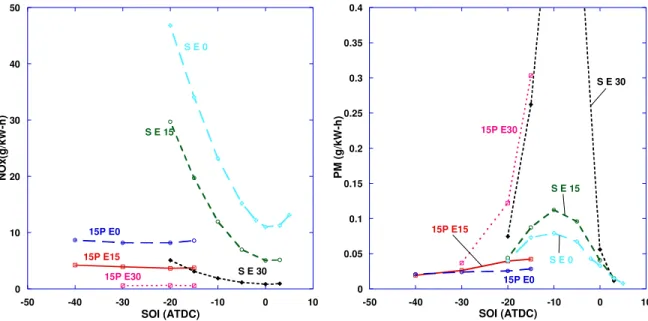
Figure 5.1 Effect of SOI on NOx and PM emissions at EGR levels 0 and 15% and 150 MPa

injection pressure. 37

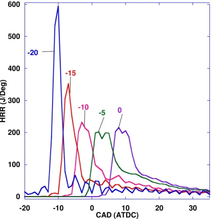
Figure 5.2 Cylinder pressure history for SOI between -20 and TDC, 0% EGR. 38 Figure 5.3 Heat release rate history for SOI between -20 and TDC, 0% EGR. 39 Figure 5.4 Effect of SOI on CO and HC emissions at EGR levels 0 and 15% and 150 MPa

injection pressure 39

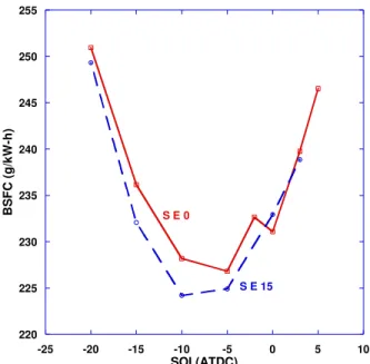
Figure 5.5 Effect of SOI on BSFC at EGR levels 0 and 15% 40

Figure 5.6 Fuel spray path at pilot SOI of -30 ATDC 41

Figure 5.7 Fuel spray path at pilot SOI of -45 ATDC 41

(8)

Figure 5.9 Effect of pilot injections (15% and 25%) on NOx and PM emissions (Main SOI 5

ATDC) 44

Figure 5.10 Effect of pilot injections (15% and 25%) on CO and HC emissions (Main SOI 5

ATDC) 45

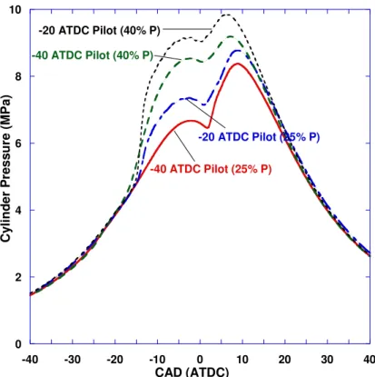
Figure 5.11 Effect of pilot injections (15% and 25%) on BSFC (Main SOI 5 ATDC) 46 Figure 5.12 Effects of pilot duration and pilot SOI on cylinder pressure 47 Figure 5.13 Effects of pilot duration and pilot SOI on heat release 48 Figure 5.14 NOx and PM emissions at different EGR levels for single and double injection

conditions at 150 MPa injection pressure 49

Figure 5.15 CO and HC emissions at different EGR levels for single and double injection

conditions at 150 MPa injection pressure 50

Figure 5.16 BSFC at different EGR levels for single and double injection conditions at 150

MPa injection pressure 50

Figure 5.17 Cylinder pressures of using the convergent nozzle with different EGR levels at

150 MPa injection pressure and –5 ATDC SOI 52

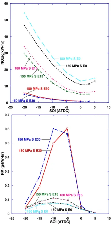
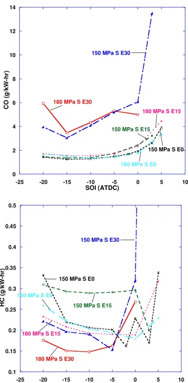
Figure 5.18 Effects of Injection pressure on NOx and PM emissions at different EGR levels 53 Figure 5.19 Effects of Injection pressure on NOx and PM emissions at different EGR levels

55 Figure 5.20 Effects of Injection pressure on NOx and PM emissions at different EGR levels

56 Figure 5.21 Comparisons of cylinder pressure at two injection pressures of 150 and 200 MPa

(9)

Figure 5.22 Comparisons of heat release data at two injection pressures of 150 and 200 MPa

at -15 ATDC and 5 ATDC SOI 57

Figure 5.23 NOx and PM vs pilot SOI at 150 MPa injection pressure (main SOI = 5 ATDC)

for different pilot fuel quantities and EGR 59

Figure 5.24 BSFC vs pilot SOI at 150 MPa Injection pressure (main SOI = 5 ATDC) 60 Figure 5.25 NOx vs PM emissions for 150 and 180 MPa injection pressures at 30% EGR for both single and double injection conditions. (Note that (-40, +5) denotes pilot SOI = -40

ATDC and main SOI = + 5 ATDC) 61

Figure 5.26 CO vs HC emissions for 150 and 180 MPa injection pressures at 30% EGR for both single and double injection conditions. (Note that (-40, +5) denotes pilot SOI = -40

ATDC and main SOI = + 5 ATDC) 62

Figure 5.27 PM and NOx emissions using the K=3 nozzle at different conditions 64 Figure 5.28 PM vs NOx for baseline nozzle (K=0) and the converging nozzle at different

conditions 65

Figure 5.29 BSFC vs NOx for the converging nozzles (K=3) in comparison with the baseline

nozzle (K = 0) 65

Figure 5.30 PM vs NOx emissions for the converging nozzles under different double

injection conditions 66

Figure 5.31 A close-up plot of Figure 5.30 with the comparison between the baseline nozzles

(K=0) and the converging nozzles 67

Figure 5.32 CO and HC emissions for the cases shown in Figure 5.31 67 Figure 5.33 NOx vs PM emissions using 10-hole injectors at different EGR levels 70 Figure 5.34 NOx vs BSFC emissions using 10-hole injectors at different EGR levels 70

(10)

Figure 5.35 NOx and PM emissions of all three injectors at 30% EGR with different

injection pressures 72

Figure 5.36 NOx and PM emissions of all three injectors at 30% EGR with different

injection pressures 73

Figure 5.37 BSFC of all three injectors at 30% EGR with different injection pressures 74 Figure 5.38 PM and NOx emissions for all the cases tested in this study (0%, 15% and 30% EGR for all three injectors at different injection pressures) 75 Figure 5.39 PM and NOx emissions for selected cases that produced emission results within

the scale shown. The number next to the data point is the SOI timing. The box on left bottom corner shows the Tier 4 standards for NOx and PM emissions 76 Figure 5.40 Cylinder pressures and normalized heat release rate data for different injectors

with 150 MPa injection pressure, 0 ATDC SOI, and 30% EGR 77 Figure 5.41 Cylinder pressure and heat release rate for 30% EGR, late injection conditions

(SOI = 2 and 3 ATDC) that produced low soot emissions shown in Figure 5.39 78 Figure 5.42 16-hole Injector geometry and a 45 degree sector mesh 79 Figure 5.43 NOx vs PM for all the single injection cases for 16 hole injectors 80 Figure 5.44 NOx vs BSFC for all the cases for 16 hole injectors 80 Figure 5.45 Cylinder pressure and HRR for three injectors (6-hole, 10-hole, and 16-hole at

150 MPa injection pressure, 0 ATDC SOI, and 30% EGR 81 Figure 5.46 CO emissions for all 16-hole injector cases 81 Figure 5.47 NOx vs PM for all the single injection cases using 6X133X480 injectors 83 Figure 5.48 NOx vs BSFC for all the single injection cases using 6X133X480 injectors 83

(11)

Figure 5.49 PM and NOx emissions for selected cases. The box on left bottom corner shows

the Tier 4 standards 84

Figure 5.50 Comparison of cylinder pressure and HRR of baseline injector (3 ATDC SOI)

and 6X133X480 (TDC SOI) injectors 86

Figure 5.51 PM and NOx emissions for selected cases that produced emission results within the scale shown. The box on left bottom corner shows the Tier 4 standards 87 Figure 5.52 Comparison of cylinder pressure and HRR of baseline and 10X133X500

injectors at 150 MPa, and 3 ATDC SOI 88

Figure 5.53 Pathway of emissions reduction 90

Figure 6.1 Surface plot of Ackley's Path Function with two variables 92 Figure 6.2 Evolution of the function value vs iteration number for the Ackley’s path function 92 Figure 6.3 Surface plot of Rastrigin’s function with two variables 93 Figure 6.4 Evolution of the function value vs iteration number for the Rastrigin’s function 94

Figure 6.5 Fitness values of all the experiments 96

Figure 6.6 Evolution of NOx, Soot, HC, and BSFC 98

Figure 6.7 Evolution of design variables 99

Figure 6.8 Schematic of double injection profile 101

Figure 6.9 Fitness values of all experiments with double injections (intake temperature 23

ºC) 103

Figure 6.10 Evolution of NOx, Soot, and BSFC values 104

(12)

Figure 6.12 Fitness values of all experiments with double injections (intake temperature 23

ºC) 106

Figure 6.13 Comparison of CO and HC emissions. On the right the fitness function included HC and CO. On the left, HC and CO emissions were not included in the fitness function

108

Figure 6.14 Evolution of NOx, PM, and BSFC values 109

Figure 6.15 Comparison of NOx and PM emissions with Tier 4 emissions 110 Figure 6.16 Fitness values of all experiments with double injections (intake temperature 40

ºC) 111

Figure 6.17 Evolution of CO, HC emissions and EGR level 113 Figure 6.18 Comparison of cylinder pressure and HRR of experiments in the first iteration

with that of experiments in last iteration 115

Figure 6.19 Comparison of fitness values and BSFC 117

Figure 6.20 Flow chart for the optimization of emissions using PSO and KIVA 120 Figure 6.21 Comparison of NOx and Soot emissions at 0, 15 and 30% EGR levels at various

SOIs 122

Figure 6.22 Comparison of cylinder pressure and heat release rate for 150 MPa, 0 SOI, and

0% EGR 123

Figure 6.23 Comparison of mean effective pressures at 0, 15, and 30% EGR levels 124

Figure 6.25 Evolution of NOx and Soot emissions 127

(13)

LIST OF TABLES

Table 3.1 Engine specifications 20

Table 4.1 Variables tested and their ranges 29

Table 4.2 Injector specifications 31

Table 4.3 Emissions standards for off-road diesel engines rated between 75 and 130 kW

(unit: g/kW-h) 31

Table 4.4 Variation of intake O2 concentration with EGR % at intake temperatures 23 °C

and 40 °C 32

Table 5.1 List of emissions and BSFC results for selected cases shown in Figure 5.25. The

EGR level was 30% for all the cases tested 62

Table 5.2 List of emissions and BSFC results for selected cases shown in Figure 5.31 using the converging nozzles. EGR level was 30% for all the cases tested 68 Table 5.3 Emissions of cases shown in Figure 5.49 at various operating conditions 85 Table 5.4 Emissions of cases shown in Figure 5.51 at various operating conditions 88 Table 6.1 Variable ranges and global minimum for Ackley's Path Function 91 Table 6.2 Variable ranges and global minimum for Rastrigin Function 93

Table 6.3 Targets used for NOx, HC, Soot, and BSFC 95

Table 6.4 Range and resolution of design variables 95

Table 6.5 Final results for single injection optimization 97

Table 6.7 Comparison of optimal point operating conditions and emissions 107 Table 6.8 Final results for double injection optimization with intake temperature 40 ºC 112

(14)

Table 6.9 Operating conditions used in the refinement of the optimum 116

Table 6.12 Operating conditions and emission results for iteration 6 130 Table 6.13 Comparison of optimal operating conditions of experiments and simulations 132

(15)

ABSTRACT

The objective of this research was to develop advanced diesel combustion strategies for emissions reduction in a multi-cylinder diesel engine. The engine was equipped with an electronically-controlled, common-rail fuel injection system, and an exhaust gas recirculation (EGR) system. This experimental setup allowed a wide range of operating conditions to be explored.

Effects of various injector parameters with various EGR levels on emissions were studied. Injector parameters included the injector flow number, nozzle hole geometry (straight, convergent), and nozzle arrangement (6-hole, 10-hole, 16-hole). The included spray angle was kept constant at 133 deg. Other engine parameters included the EGR rate (0-41%), injection pressure (150-225 MPa), start of injection (SOI) (-20 to 5 ATDC), start of pilot injection (-40 to -15 ATDC), and pilot fuel percentage (0-25%).

For single injection operations, a simultaneous reduction of NOx and particulate matter (PM) was achieved by using high EGR (30%) with late injection timing (0 to 5 ATDC) at high injection pressures (150 MPa). For double injection operations, NOx and PM emissions were reduced using 30% EGR, 15% pilot injection at an early pilot timing (-30 ATDC) and late main injection (5 ATDC).

Injectors with low flow numbers were able to produce low emissions at high EGR levels (>35%) and high injection pressures (>150 MPa). The combustion was stable at these high EGR levels as the SOI was held at 0 ATDC. On the other hand, injectors with high flow numbers were not able to produce stable combustion at such high EGR levels with late SOI.

(16)

Small nozzle holes in the 10-hole injector helped reduce NOx and PM emissions significantly. However, a 16-hole injector with a similar nozzle hole diameter produced very high PM emissions due to poor air utilization.

To improve the speed of optimization for lower emissions, particle swarm optimization (PSO), a stochastic, population-based evolutionary optimization algorithm, was applied to both engine experiments and numerical simulation. The algorithm was tested using test functions that were used in the field of optimization to ensure reaching a global optimum. A merit function was defined to help reduce multiple emissions simultaneously. The PSO was found to be very effective in finding the optimal operating conditions for low emissions. The optimization usually took 40-70 experimental runs to find the optimum. High EGR levels, late main injection, and small pilot amount were suggested by the PSO. Multiple emissions were reduced simultaneously without a compromise in the brake specific fuel consumption. In some cases, the NOx and PM emissions were reduced to as low as 0.41 and 0.0092 g/kW-h, respectively. The operating conditions at this point were 34% EGR, 5 ATDC main SOI, -24 ATDC pilot SOI, and 5% pilot fuel.

The PSO was also integrated with an engine simulation code and applied to engine optimization numerically. The results showed that optimization of engine combustion using PSO with numerical simulation was an effective means in the development of future emission reduction strategies.

(17)

ACKNOWLEDGEMENTS

I would like to take this opportunity to express my gratitude to my major professor and adviser Dr.Song-Charng Kong for providing me an opportunity to work under his supervision. I also would like to thank him for providing timely help, feedback, and for motivating me to pursue my interests. I am also thankful to my POS committee members Dr. Terry R. Meyer, Dr. Michael G. Olsen, Dr. Hui Hu, and Dr. Stuart J. Birrell for serving in my dissertation committee, giving special effort and time to review my dissertation and providing useful suggestions and comments.

I would also like to acknowledge the financial and material support by John Deere. Their help in identifying the problem and setting up the laboratory is greatly appreciated.

This section would not be complete without acknowledging many people who have helped me in finishing this work. I would like to thank Jim Dautremont for his help in building the test cell and for providing valuable suggestions. In addition, I also would like to thank undergraduate students Travis Whigham, Derek Mullins, Nathan Uelner, Lukas Jon Shea for their dedicated work in the engines lab spending countless hours building the test cell. This work would not have been possible without their efforts. I would like to specially thank Noah Van Dam for his diligent work related to PSO and model calibrations. Finally, I would like to thank all members of Dr.Kong’s research group and my colleagues at Iowa State University for all the help they have provided.

(18)

CHAPTER 1. INTRODUCTION

1.1 Background

Since its invention in late 1800s, the internal combustion (IC) engine has had a significant impact on society and has been the foundation for the successful development of many commercial technologies. It is reported that approximately 301 million automobiles are powered by IC engines worldwide in 2008 [1]. IC engines can deliver power in the range from 0.01 kW to approximately 20X103 kW, based on their displacement. This flexibility allows IC engines to be used in various applications such as automobiles, trucks, locomotives, marine, aircrafts, and power generation. Because of its widespread applications and ages, the IC engine industry is very large and competitive [2].

Population and economic growth are usually the fundamental drivers of the energy demand. The overall energy need can be divided into four demand sectors. They are power generation, transportation, industrial, and residential. It was reported that each of these major demand sectors will experience considerable growth through 2030 [3]. The anticipated volume growth is the highest for the power generation sector followed by transportation sector. In the transportation sector, personal transportation, transportation of goods, non-road works such as construction and agriculture are mostly provided by IC engines. As the environmental concern rises and the demand for low-emissions vehicles increases, it has become a priority for the industry and scientific community to meet these challenges.

The diesel, i.e., compression-ignition (CI), engine is the prime power source in the transportation sector as it offers better fuel economy, power, and durability over the gasoline, i.e. spark-ignition (SI), engines. Approximately 94 percent of all freights in the U.S. are

(19)

moved by diesel power. Diesel engines are also the primary power source for non-road equipment including construction and agricultural equipment, marine vessels, and locomotives. While diesel engines are known for their efficiency and durability, they have certain environmental disadvantages over gasoline engines.

1.2 Motivation

The United States is the world’s biggest consumer of oil, and over half of the oil is imported. Such dependence on foreign oils can lead to the national security issue. Thus, improving IC engine efficiency is important in reducing foreign oil dependency. Improving engine efficiency can also help reduce emissions of carbon dioxide (CO2), which is a greenhouse gas although it is a complete combustion product.

Four major engine exhaust pollutants are carbon monoxide (CO), nitrogen oxides (NOx), hydrocarbons (HC), and particulate matter (PM) (also called soot). Of these emissions, SI engines emit significantly less PM than CI engines as fuel-air mixture in SI engines is homogeneous and combustion is stoichiometric. A three-way catalyst can be used to convert about 90-95% of CO, HC and NOx into CO2, H2O, and N2. On the other hand, non-homogeneous combustion in CI engines results in a diffusion flame that leads to high NOx emissions, and the fuel rich region inside the jet leads to PM formation. However, CI engines do not emit as much CO and HC as SI engines because CI engines are operated in overall lean conditions and there is oxygen available to prevent incomplete combustion.

Research found that PM are carcinogenic and can elevate lung cancer rates in occupational groups exposed to diesel exhaust [4, 5]. NOx emissions can form nitric acid which contributes to acid rain. NOx will also react with volatile organic compounds in the

(20)

presence of sunlight to form ozone, a key component of smog. It was also reported that NOx can deplete the ozone layer at high altitudes and make the earth vulnerable to many kinds of harmful solar rays [6]. Regulations on engine exhaust emissions and fuel economy are now enforced around the world. The emission standards have been categorized according to the type of the engine, engine size, and its application.

There have been many studies on in-cylinder combustion to reduce diesel engine emissions. Simultaneous reduction of PM and NOx emissions from diesel engines is the biggest challenge faced by the industry. In order to reduce the NOx emissions, the local combustion temperature has to be kept below 2200 K, but PM emissions will increase at these reduced temperature levels. However, when the temperature is below 1650 K, both NOx and PM can be reduced simultaneously. This concept is referred to as low temperature combustion (LTC). Fuel injection plays an important role in determining the emissions. Oftentimes, the combustion is not sustainable and the brake power is reduced significantly when the engine is operating under LTC regimes. Modifying the fuel injection can improve the combustion stability while operating under LTC regimes. This study will explore LTC operation in diesel engines using various fuel injection strategies for reducing exhaust emissions while maintaining comparable engine efficiency.

1.3 Objectives

The objective of this research is to investigate the effect of different fuel injection strategies and engine operating parameters on diesel emissions. This study will also develop a methodology to optimize the operating parameters in order to meet the future emissions standards.

(21)

Previous studies showed that, depending on the injection strategy, exhaust gas recirculation (EGR) could be used to reduce NOx emissions [7]. Multiple fuel injections in conjunction with EGR was also found to reduce PM and NOx emissions simultaneously [8]. However, only limited literature is available on the effects of injector geometry on engine performance.

In this study, several approaches are introduced to improve the diesel combustion pattern to reduce primarily NOx and PM emissions. First, engine experiments were performed on a multi-cylinder diesel engine using baseline injectors. Then injectors with various nozzle geometries and sizes were tested to study their effects on emissions reduction. Performance of different injectors under various EGR, injection pressure, and double injection conditions was evaluated.

Response surface equations for NOx, PM and brake specific fuel consumption (BSFC) were derived to study effects of different variables on emissions. Interactions between these variables were also studied to determine the combined effect of variables on emissions. While response surfaces can predict the trend of emissions, they often failed to find the global optimum particularly when the surface is multi-dimensional. As it is impossible to test all the possible operating conditions on an engine, a particle swarm optimization (PSO) method will be used to optimize the operating conditions to reduce emissions.

(22)

CHAPTER 2. LITERATURE REVIEW

Diesel engines can offer better fuel economy and durability as compared to gasoline engines. While the high efficiency of diesel engines can benefit CO2 emissions reduction, their PM and NOx emissions are subject to legislative limits due to their adverse effects on human health and environment. In the mean time, legislations also mandate the emissions of CO and HC [9].

Diesel combustion can be manipulated by many parameters such as EGR, injection pressure, and the injection profile. All these parameters will affect the combustion process, which in turn determines the emissions levels. Parameters which affect the combustion process are briefly explained below, followed by discussions on methods of optimizing engine performance for emissions reduction.

2.1 Exhaust Gas Recirculation (EGR)

A fraction of the exhaust gas are re-circulated from the exhaust to the intake system. This recycled exhaust is mixed with fresh intake air before the intake air enters the cylinder. It has been shown by previous studies that EGR can reduce NOx emissions by reducing the combustion temperature [10]. The NOx emissions are formed inside the cylinder at high temperature regions. According to the equation Q= m.Cp.∆T, the total temperature increase (∆T) is affected by the specific heat (Cp) of the constituents of the gas. If the specific heat of the gas is higher, then the temperature increase of the gas will be reduced to keep the total heat release (Q) constant. The specific heat of water vapor (H2O) and carbon dioxide (CO2) are considerably higher than the specific heat of fresh air. When exhaust gas (containing H2O and CO2) is introduced into the cylinder, a lower gas temperature can be obtained leading to

(23)

a lower local combustion temperature and a reduction in total NOx. In the same time, oxygen availability is reduced when EGR is used. Reduced oxygen availability also reduces the NO formation as explained by Eq. (2.1), (2.2), and (2.3) below. The formation of NOx emissions can be described by the extended zeldovich mechanisms [11].

O + N2 NO + N (2.1) N + O2 NO + O (2.2)

N + OH NO + H (2.3)

The combined effect of equivalence ratio (Φ) and temperature (T) on soot and NOx formation was explained by Kamimoto and Bae [12] based on detailed chemistry modeling. In this study, a quantitative Φ-T map was created for NOx and soot by performing 0-D chemical kinetics calculations. The NOx and soot formation with respect to Φ and T are depicted in Figure 2.1. It can be seen that soot formation occurs under rich conditions (Φ > 2) and temperature between 1700 and 2100 K. On the other hand, NOx is formed when combustion temperature is above 2200 K for Φ< 2.

(24)

Figure 2.1 Soot and NO concentrations without EGR as a function of the equivalence ratio and temperature. Soot is in g/m3, NO in mole fractions, and temperature in K.

The line in Figure 2.1 corresponds to the adiabatic flame temperature of diesel fuel with respect to the equivalence ratio. It can be noted from the figure that the adiabatic flame temperature needs to be less than 2200 K to avoid the NO formation at low equivalency ratios. At higher equivalence ratios, the temperature needs to be further reduced to avoid the formation of soot. If the temperature is kept below 1650 K, both NOx and soot formation can be avoided regardless of equivalence ratio. Figure 2.2 shows three adiabatic flame temperature paths for different compression ratios with 60 % EGR. The adiabatic flame temperatures shifted towards left with the use of EGR. As it can be seen from Figure 2.2, both NOx and soot are avoided by reducing the adiabatic flame temperature.

(25)

Figure 2.2 Soot and NO concentrations with 62% EGR as a function of equivalence ratio and temperature. Soot is in g/m3, NO in mole fractions and temperature in K.

Exhaust gases (primarily CO2 and H2O) have higher specific heat (Cp) compared to the fresh intake air. This effectively reduces the combustion temperature and reduces the formation of NOx. There have been many studies on the effect of EGR on NOx and PM emissions in diesel engines. It was shown experimentally that EGR can reduce the oxygen flow rate to the engine [13]. This results in a reduced local flame temperature during combustion and, thus a reduced rate of NOx formation.

In addition to lowering the combustion temperature, EGR was also found to retard the start of combustion and alter the emission characteristics [14]. The delayed ignition has two advantages. It can reduce the cylinder pressure rise rates, which can reduce the combustion

(26)

noise as well as increase the mixing time, which can create more homogeneous mixture for PM reduction [15, 16].

2.2 Injection Pressure

The use of ultra high injection pressure can reduce the PM emissions. High injection pressure combined with micro-hole nozzle increases turbulent mixing for better fuel vaporization and PM reduction [17]. High injection pressure reduces the injection duration. Reduction in injection duration allows more time for fuel-air mixing to obtain a more homogeneous mixture. Better mixing leads to higher oxidation of PM and a reduction in the total PM emissions [18, 19]. However, due to high combustion temperatures associated with using high injection pressures, NOx formation increases. The use of EGR along with high injection pressure can reduce NOx formation while reducing PM [20]. Due to better atomization, CO and HC emissions can also be reduced. A small increase in BSFC was observed when high injection pressure was used. This is due to the increase in pump losses as the fuel pump is needed to increase the rail pressure.

2.3 Injector Geometry

The geometry of the nozzle in an injector plays an important role in controlling diesel spray atomization and combustion. Several nozzle parameters such as the nozzle hole diameter, the length-to-diameter ratio, and the roundness of the nozzle inlet will affect fuel atomization characteristics and combustion [21, 22]. The importance of the nozzle flow and its effects on spray atomization were discussed by Bergwerk [23]. Internal flow phenomena such as the velocity distribution inside the nozzle, turbulence, and cavitation inside the

(27)

nozzle can determine the disturbance level in the liquid jet at the nozzle exit

initial disturbances will affect the liquid breakup, penetration, spray evaporation, and eventually ignition and combustion.

piston in a diesel engine togeth

Figure 2.3 Fuel injector and diesel spray in a diesel engine.

Nozzles with large diameters are less efficient in atomizing fuel sprays compared to those with smaller diameters. However, small nozzles require

which could reduce combustion efficiency

can reduce the injection duration of small diameter nozzles by increasing the injection velocity.

The nozzle size will influence the fuel performance and emissions [27]

hole diameter on PM formation in diesel engine environments. Nozzles with different diameters were tested in a constant volume

reduced as the nozzle diameter was reduced. Numerical modeling using detailed also revealed that PM formation can be closely related to the lift

nozzle can determine the disturbance level in the liquid jet at the nozzle exit

initial disturbances will affect the liquid breakup, penetration, spray evaporation, and eventually ignition and combustion. Figure 2.3 depicts a typical combustion

together with a high speed image of diesel spray.

Figure 2.3 Fuel injector and diesel spray in a diesel engine.

Nozzles with large diameters are less efficient in atomizing fuel sprays compared to those with smaller diameters. However, small nozzles require a longer injection duration which could reduce combustion efficiency [26]. High injection pressures (150

can reduce the injection duration of small diameter nozzles by increasing the injection

The nozzle size will influence the fuel–air mixing process and therefore engine [27]. Pickett and Siebers [17] investigated the effects

formation in diesel engine environments. Nozzles with different diameters were tested in a constant volume chamber. It was found that PM

reduced as the nozzle diameter was reduced. Numerical modeling using detailed

formation can be closely related to the lift–off length of the diesel nozzle can determine the disturbance level in the liquid jet at the nozzle exit [24, 25]. These initial disturbances will affect the liquid breakup, penetration, spray evaporation, and combustion chamber and a

Figure 2.3 Fuel injector and diesel spray in a diesel engine.

Nozzles with large diameters are less efficient in atomizing fuel sprays compared to a longer injection duration ures (150 – 200 MPa) can reduce the injection duration of small diameter nozzles by increasing the injection

air mixing process and therefore engine investigated the effects of nozzle formation in diesel engine environments. Nozzles with different formation can be reduced as the nozzle diameter was reduced. Numerical modeling using detailed chemistry off length of the diesel

(28)

spray [28]. Meanwhile, the PM–NOx trade–off can be overcome by using high exhaust gas recirculation (EGR) to achieve low temperature combustion.

Another important characteristic of a nozzle is the variation in the nozzle cross– sectional area along its length. This geometrical characteristic can be defined by the conicity of the nozzle which is also called K–factor,

K 100 ·

(2.3)

where Di is the inlet diameter, Do outlet diameter, and L the length of the nozzle.

Various studies have showed that the variation in the nozzle geometry can produce different fuel spray characteristics [21, 22, 29, 30]. Nurick [31] investigated the effect of nozzle inlet geometry on the nozzle flow. It was found that cavitation can be prevented by using a round–edge inlet nozzle with the ratio of inlet radius to nozzle diameter (R/D) larger than 0.14. Benajes et al. [32] conducted an experimental study to analyze the influence of different orifice geometries (conical and cylindrical) on the injection rate of a common–rail fuel injection system. It was found that the discharge coefficient was higher in the conical nozzle than that in the cylindrical nozzle. In addition, the flow in the cylindrical nozzle collapsed at high injection pressures due to cavitation that was not observed in the conical nozzle.

Literature on the effects of nozzle conicity on spray related issues such as cavitation and injection velocity is limited. Desantes et al. [33] tested three injector nozzles with different conicity ( K = –0.2, 0, 1.1) for cavitation under different injection pressures and ambient pressures. Fuel flow rates and momentum fluxes at the nozzle exit were measured. The injection pressure was varied between 2 and 160 MPa.

(29)

It was found that, as K–factor increased, the tendency towards cavitation was reduced [33]. Cavitation was not evident for K=1.1. The mass flow rate can be reduced due to cavitation at high injection pressures. The momentum flux did not change as the K–factor of the nozzle changed, i.e., cavitation did not influence the momentum flux. Hence, the exit velocity was increased to compensate the reduced mass flow rate due to cavitation.

2.4 Double Injections

Splitting the injected fuel into a number of pulses can cause a change in the combustion characteristics. Appropriate configurations of multiple injections have shown to decrease PM emissions without a significant increase in NOx emissions. The availability of local oxygen can be improved greatly when fuel is injected multiple times. This is due to an increase in mixing time of air and fuel. An increase in local oxygen concentrations increases the oxidization of PM, leading to reduced PM emissions. Some optimal injections were found to have more fuel in early injections and less in subsequent injections [34-36]. These findings agree with results of Benajes et al. [37] who demonstrated that by using a post injection strategy, reduction in PM could be achieved without compromising NOx emissions or fuel consumption. Optimal injection strategies can be different for different operating conditions.

2.5 Optimization

Optimization is a process of maximizing or minimizing a mathematical function, an output of a process, or an objective function based on input variables that affect the process. Depending on the complexity of the function, many different types of optimizations can be

(30)

used. If the function can be expressed in the form of a mathematical function, differential calculus can be used to minimize or maximize the function [38]. However, there are several problems whose topology cannot be expressed in the form of a mathematical function. In such cases, methods such as response surface method (RSM), genetic algorithm (GA), and particle swarm optimization (PSO) can be used to examine the peaks and valleys of the design hyperspace.

Internal combustion engine operation is a good example of a system where the interaction between engine operating parameters (also called design variables) is so intertwined that a reliable response surface model is not available [39]. Particle swarm optimization (PSO) is a stochastic, population based evolutionary algorithm which can be used to find the maximum or minimum of a given function. RSM, GA, and PSO are explained below.

2.5.1 Response Surface Method

Response surface methodology comprises a group of statistical techniques for building of empirical models and model exploitation. By careful analysis of experiments, it creates a response, or a mathematical equation depicting the design variables and their interactions [40]. Once the response is created, search of the objective function hyperspace is started from one point to another. The direction of the optimization is determined by the direction of steepest decent for minimizing the objective function [41, 42]. This method is also called gradient search method.

Gradient search methods are applied to the response surface model to determine the path of steepest decent, which points in the direction of reducing the objective function value.

(31)

By following this path, the objective function will eventually downturn after reaching a local valley. At the valley, another factorial is applied to again investigate the local terrain. If another hyper plane with a discernable gradient can be applied, the optimization continues. If the response surface no longer appears planar, or appears relatively non-sloped, a local minimum is likely to exist nearby, and additional experiments with high resolution are performed to develop a curved surface model which is more accurate than the original model. This surface can then be searched with traditional mathematical methods [43].

This method is effective in finding a local minimum. However, it does not promise a global minimum. A good judgment on the part of the user is required to start the process at a good starting point. Starting at a poor point may result in finding only a local minimum if there is one in the vicinity [44]. In a study performed using response surface to optimize the engine emissions, it was reported that a good starting point was chosen which lies near the previously known optimum point [45]. In this study, a mathematical expression consisting of the several emissions is used as an objective function. This simplified the complicated problem of reducing different emissions into a search for maximization of the objective function.

2.5.2 Genetic Algorithm

Genetic algorithm is a search technique used to find exact or approximate solution of a given optimization problem. GA is a class of evolutionary algorithms inspired by evolutionary biology such as mutation, selection and crossover. A population that includes randomly selected citizens is allowed to evolve under pre-determined selection rules to maximize the fitness. Each citizen representing the input factor level is represented as a

(32)

sequence of 0’s and 1’s (binary encoding). Fitness value of each citizen is evaluated and fittest citizens are allowed to breed with some randomness to generate a new generation of citizens [46, 47].

Based on the differences in the application of mutation, GA can be divided into two distinct types, the simple GA and the micro-GA (µGA). The simple GA utilizes a population size of around 200 citizens in each generation [46]. If this type of GA is used, then few generations would require thousands of function evaluations. This method would be prohibitive when each function evaluation takes significant amount of time for experimental engine runs or 3-D computer simulations. A µGA on the other hand utilizes only around 5 individual citizens in each generation. The population is expected to converge relatively quickly. Several modifications such as elitism are used in combination with µGA to increase the likelihood of finding a global optimum while exploring throughout the search space.

The µGA was used by some researchers to reduce the engine emissions by optimizing the engine operating conditions. These studies included using the µGA on an experimental engine and 3D computer simulations. An experimental study done by Thiel et al. was able to meet the 2002/2004 emissions levels in a single cylinder experimental diesel engine [48]. In a similar study done by Liechty et al. in 2004, a single cylinder engine was coupled with µGA using a computer interface to automate the experiments. Several input variables including start-of-injection, EGR, boost pressure, multiple injection parameters were optimized to reduce the emissions. The optimum point was found in 31 generation with 5 citizens in each generation. The optimum resulted in emissions that had 2 times higher PM and NOx emissions compared to the 2007 EPA standards, but with an 8% reduction in fuel consumption [49].

(33)

2.5.3 Particle Swarm Optimization

Particle swarm optimization (PSO) is a stochastic, population based evolutionary algorithm for problem solving. This method was proposed in 1995 by social-psychology major James Kennedy and electrical engineer Russell Eberhart. PSO has roots in two main component methodologies. One is its ties to artificial life in general, and to bird flocking, fish schooling, and swarming theory in particular [50]. It is also related to evolutionary computation, and has ties to both genetic algorithms and evolutionary programming. Implementing PSO is computationally inexpensive in terms of memory and speed as it requires only primitive mathematical operators. Early tests have found the implementation of PSO to be effective with several kinds of problems. PSO has also been demonstrated to perform well on test functions used for validating genetic algorithm optimization [50, 51].

In theory, individual members of a school or a swarm can profit from discoveries and previous experience of all other members during search for food. During the original experiments with PSO, birds exhibited “flocking” characteristics such as synchronously changing direction and scattering and regrouping. This suggests that social sharing of information among co-existing members offer an evolutionary advantage [52, 53]. This hypothesis is fundamental to the development of PSO.

This model also contains an attraction factor to a roosting area. In these simulations, birds will begin to fly around without a particular destination and then spontaneously form flocks. This goes on until one bird fly over the roosting area. When the programmed “desire to roost” is higher than the “desire to stay in flock”, the bird will pull away and land.

(34)

A swarm of members is analogous to a set of design points and a design space. The position of a design point is influenced by defined neighbors. The “velocity” (speed and direction) of a design variable at the beginning of an iteration is given by:

Vi+1 = Vi + C1R1 (Pbesti – Xi) + C2R2 (Gbest – Xi) (2.4)

The “velocity” will be used to determine the new value of a design variable as given below:

Xi+1 = Xi + Vi+1 (2.5)

X is a design variable, i is the design variable number, R1 and R2 are random numbers between 0 and 1, C1 and C2 are constants (generally 2.0), Pbesti is the best value found by the design variable i, and Gbest is the best value in all previous iterations of any design variable (i.e. swarm member).

Attributes of particles are given as follows:

- Location of particle in the design space (i.e. co-ordinate or design variable value) - Objective function value

- Velocity vector value - Pbest

- Pbestold (Pbest from previous iteration)

The search for the optimal value is controlled in PSO by three different expressions. Vi+1 = Vi + C1R1 (Pbesti – Xi) + C2R2 (Gbest – Xi) (2.6)

Momentum

Exploration term

(35)

The momentum term keeps the velocity (value of design variable in the next iteration) from changing abruptly. The exploration term (Pbest) learns from its own experience from previous iterations. The exploitation term (Gbest) term learns from collaboration from all other members and all previous iterations. A limit on velocity (V) is enforced (Vmax) to restrict the value of design variable from going beyond the range of that design variable.

An inertia weight has been applied to Eq. (2.4) to control the impact of a particle’s previous velocity on the calculation of the current velocity vector. The modified equation is shown in Eq. (2.7).

Vi+1 = Winer(Vi + C1R1 (Pbesti – Xi) + C2R2 (Gbest – Xi)) (2.7)

A large value for Winer facilitates global exploration, which is particularly useful for

problems with complex design spaces. A small value allows for more localized searching, which is useful as the swarm moves toward the neighborhood of the optimum [54, 55]. A large value of 0.729 calculated using constriction factor method was used in this study to facilitate a global exploration of search space. The flow chart of PSO is given in Figure 2.4.

(36)

Figure 2.4 Flow chart of PSO optimization methodology.

Initialize population with random positions

Evaluate each member’s objective function value (Fitness)

Compare each member’s fitness to its Pbest (calculate Pbest)

Identify particle in the neighborhood with best success so far and make it

Gbest (calculate Gbest)

Update particle’s velocity and position (Eq. 2.4 & 2.5)

Converged

Exit Yes No

(37)

CHAPTER 3. EXPERIMENTAL SETUP

Experiments were performed in this study using a John Deere 4045HF475 off-road four-cylinder 4.5 L engine. The engine is rated at 129 kW at 2400 rpm. Detailed engine parameters are given in Table 3.1.

Table 3.1 Engine specifications

Engine John Deere 4045 HF475

4-cylinder 4-valve direct injection Bore and Stroke (mm) 106 x 127

Total engine displacement (L) 4.5

Compression Ratio 17.0:1

Valves per Cylinder 2 / 2

Firing Order 1-3-4-2

Combustion System Direct Injection

Engine Type In-line, 4-stroke

Aspiration Turbocharged (located on engine)

Injection System Common Rail

Piston Bowl-in-piston

3.1 System Layout

The layout of the experimental setup used to conduct the experiments is shown in Figure 3.1. The exhaust line was divided into two pipes to drive the EGR. A suction pump that is placed in the EGR loop sucks the exhaust into the EGR line. The engine was controlled by the DevX software provided by John Deere. The engine was coupled with a DC dynamometer manufactured by GE and controlled by a standalone dynamometer controller. Details of the system components will be discussed in the following sections.

(38)

(39)

Figure 3.2 Picture of the engine facility.

3.2 Measurement Techniques

The following sections explain the instruments and procedures used for measuring the various performance parameters. All the experiments were performed at steady-state conditions when there was no change in engine oil temperatures and exhaust gas temperatures. The engine was warmed up at the beginning of each test to reach steady-state conditions.

EGR Setup

EGR Coolers

Engine

control Unit

John Deere 4045 Engine

(40)

3.1.1 Intake Air Flow Rate Measurement

The intake air flow to the engine was measured using a Meriam laminar flow element (LFE) model 50MC2-4. The calibration on the unit was performed according to NIST standards. The calibration data were standardized to an equivalent dry gas flow rate at 70º F and 29.92 in Hg absolute (101.3 kPa abs). The LFE measures the actual volumetric flow rate. To obtain the actual volumetric flow rate, the differential pressure (DP) across the LFE to the LFE was measured. The flow rate was obtained by substituting the DP value into Eq.(3.1).

Flow rate CFM B DP C DP _(3.1)

where B is 5.3518E+01 and C is -9.64278E-02.

3.1.2 Cylinder Pressure Measurement

An uncooled and ground insulated engine pressure transducer manufactured by Kistler (6125 A) was used to measure the cylinder pressure during engine operation. The cylinder pressure acts on the diaphragm which converts the pressure into a proportional force inside the sensor. This force is then transferred to the quartz package, which produces an electrostatic charge under load. An electrode taps off this charge and feeds it to the connector, where it is converted into a voltage by a charge amplifier connected in series. The crank shaft position was measured using an optical encoder attached to the engine crank shaft wheel. The resolution of the optical encoder was set to 0.25 crank angle degree (CAD) resolution. A trigger was used to synchronize the cylinder pressure measurement and the crank shaft position.

The cylinder pressure at the first data point was taken as a reference voltage each time the cylinder pressure was measured at BDC of the intake stroke, where it was assumed that

(41)

the cylinder pressure was equal to the intake boost pressure. The remaining voltage data were collected in reference to this first point. If the cylinder pressure at a certain point is greater than the first point, then the voltage at that point would be higher than the reference voltage. The following equation was used to convert the voltage data into absolute pressure.

P V V_! C. C P#$ (3.2)

where Pi is the cylinder pressure at point i in psi, Vi is the voltage recorded at point i in volts, V1 is the voltage at a reference point in volts, C.C is the calibration constant for the cylinder pressure transducer (psi/volt), Pint is the intake boost pressure (also the pressure at the reference point) in psi. To calculate the ensemble average, the data points for all the acquired engine cycles that were associated with each crank angle were added and averaged for over 50 cylinder cycles.

3.1.3 Gas Emissions Measurement

The gaseous emissions were measured using the HORIBA 7100 DEGR emissions analyzer. The analyzer and exhaust gas flow inside each unit were controlled by the main control unit (MCU). CO, CO2, and EGR CO2 emissions were measured using AIA-722 series analyzers. These analyzer use a non-dispersive infrared absorption (NDIR) method for measuring CO and CO2. A non-heated exhaust gas sample was dried in the sample handling system before flowing into the analyzer. In the NDIR analyzer, two equal-energy infrared beams are directed through two parallel optical cells. One of them is for reference and another for sample measurement. When the sample is flown through the analyzer, certain wavelengths in the infrared beam are absorbed by the component of interest in the sample

(42)

gas. The quantity of infrared radiation that is absorbed is proportional to the component concentration.

NOx was measured using a chemiluminescence sensor (CLD) (CLA-720MA). Before the sample is sent to the analyzer, the sample is led through a catalyst which converts NO2 in the sample to NO. After the conversion, the sample is exposed to ozone which results in a chemiluminescent reaction yielding NO2 and oxygen. This reaction produces light which has intensity proportional to the mass flow rate of NO into the reaction chamber. The light is measured by means of a photodiode and associated amplification electronics.

The total hydrocarbons (HC) were measured using a heated flame ionization detector (FID) analyzer (FIA-725A). The ionization mechanism in the analyzer is carried out in two phases. In the first step, organic compounds in the sample are cracked to form CH, CH2, and CH3 radicals. In the second step, these radicals react with oxygen to form CHO+ and an electron (e-). The electrometer in the analyzer measures the current generated by the ionization of the carbon atoms in the flame fueled by a 40% hydrogen (in helium) and air mixture. The current generated is proportional to the total hydrocarbon content in the sample.

3.1.4 PM Measurement

An AVL smoke meter (415 S) was used to measure PM in the exhaust. The heated sample probe takes the sample from the exhaust pipe into the analyzer. The sample is then passed through a filter paper. The degree to which the filter paper is blackened indicates the PM content in the sample. The paper blackening is measured using an optical reflectometer head. PM in the sample is zero for white filter paper and 10 for completely black paper. The

(43)

paper blackening increments are linear between white and black. The filter soot number (FSN) is calculated by the instrument using Eq.(3.3).

FSN 10 · 1 '(

') (3.3)

Based on the FSN and the volume of the sample taken, FSN is converted by the instrument using built-in correlations to mg/m3.

3.1.5 EGR Measurement

A low pressure loop was used to re-circulate the exhaust gas into the intake manifold. The exhaust gas was driven into the intake using the vacuum created by a suction pump. The exhaust gas was cooled using an intercooler before it reaches the vacuum pump. The exhaust gas is allowed to mix with intake air. The mixture then goes through the compressor of the turbocharger. The supercharger was driven using an AC motor whose speed was controlled by a frequency inverter. The EGR level in the intake was measured using following formula.

EGR % ./01234567 ./012548

./0129:;5<=4 ./012548 (3.4)

3.1.6 Exhaust Flow Rate Calculation and PM Unit Conversion

As mentioned above, PM was measured in the units of mg/m3. Tier 4 emissions standards set by environmental protection agency (EPA), however, mandate all emissions in g/kW-h. This necessitates the conversion of PM emissions from mg/m3 to g/kW-h. Exhaust

volumetric flow rate (>?_@ is required to do such a conversion. The exhaust mass flow rate was calculated by adding the flow rates of intake air and fuel. The ideal gas law was used to calculate the volume flow rate of the exhaust. PM was then calculated using following formula.

(44)

PM g kW h⁄ PM g m_{⁄ V?}G _H !

IJKLM NOPMJ (3.5)

Exhaust temperature measured after the turbocharger was used in the ideal gas law equation. Universal gas constant was calculated using R = 8.314/MWE. Molecular weight of exhaust (MWE) was calculated using the concentrations of the gases recorded by the Horiba analyzers in order to evaluate the universal gas constant.

3.1.7 Emissions Unit Conversion

During the emissions measurement, a predetermined amount of exhaust sample was fed to the analyzers. The analyzers measure concentration of the emissions in ppm (parts per million). However, the EPA emissions standards require that all emissions are reported in the units of g/kW-h. The SAE standard SAE J1003 recommends a procedure to covert the diesel engine emissions from ppm to g/kW-h. As this standard requires, all emissions are measured at steady state operating conditions. Exhaust flow rate was used to convert the units of emissions from ppm to g/h. This was divided by the brake power of the engine to convert the units to g/kW-h. Equations 3.6-3.11 were used to convert the units of emissions from ppm to g/kW-h. HC g h⁄ RS/ !T⁄ UV WX /0 !T_⁄ U_{Y /0}₁_{Y S/ !T}_⁄ U (3.6) CO g h⁄ W[\RS/ !T⁄ UV WX W]Y αW_^ ./0 !T⁄ UY /0₁Y S/ !T⁄ U2 (3.7) NO_{_} g h⁄ W`\1Ra0:⁄!TUV WX W]Y αW_^ ./0 !T⁄ UY /0₁Y S/ !T⁄ U2 (3.8)

(45)

BSHC _{IJKLM NOPMJ}S/ b c⁄ (3.9)

BSCO _{IJKLM NOPMJ}/0 b c⁄ (3.10)

BSNO_ _{IJKLM NOPMJ}a0: b c⁄ (3.11)

3.1.8 Heat Release Rate Calculation

Heat release rate (HRR) inside the cylinder was calculated based on the principle that the apparent net heat release rate, which is the difference between the apparent gross heat release rate and the heat transfer rate to the walls, equals the sum of rate at which work is done on the piston and the rate of change of sensible internal energy of the cylinder contents. The following three assumptions were made in calculating the HRR. First, the gas mixture inside the cylinder is assumed to be homogeneous. Second, the gases inside the cylinder obey the ideal gas law. Third, the specific heat (γ) of the charge mixture is constant throughout the combustion. The heat transfer to the wall was calculated by assuming the cylinder wall temperature as 600 K. The HRR was calculated using Eq.(3.12).

de3 dθ γ γ !· p · dg dθ ! γ !· V · dN dθ HL (3.12) where de3

d$ is the net heat release rate, γ is the ratio of specific heats (Cp/Cv), V is the

instantaneous cylinder volume, dg

dθ is the rate of change of cylinder volume with respect to

crank angle, p is the instantaneous cylinder pressure, dN

dθ is the rate of change of cylinder

(46)

CHAPTER 4. METHODS AND PROCEDURES

All the experiments were performed at 1400 rpm which is the engine speed that produces the peak torque. Ultra-low sulfur No. 2 diesel fuel was used for all the engine experiments. Table 4.1 gives detailed descriptions and respective ranges of the engine operating variables that were tested. The start of injection (SOI) is denoted in degrees after Top Dead Center (ATDC). Most of, but not all, the combinations were tested, as either combustion did not sustain at certain cases or it was not necessary to test certain conditions due to apparently high emissions. A fuel mass of 50 mg/injection was injected. The engine was controlled and monitored using DevX software provided by John Deere.

Table 4.1 Variables tested and their ranges

Main SOI -20 to 5 ATDC Start of Injection Pilot SOI -40 to -15 ATDC Start of Pilot Injection

EGR 0% to 40% % of EGR

Injection pressure 100 to 200 MPa Pressure at which fuel is injected

Pilot fuel 15%, 25%, 40% % of total fuel that was injected during pilot injection.

4.1 Injector Selection

An injector is identified by three numbers, eg., 6X133X800. The first number indicates the number of holes in the injector. The idea behind using multiple nozzles in an injector was to utilize the air in the cylinder more effectively. Multiple holes can also increase the total fuel injected at a given injection pressure. The nozzles on the tip of the injector are uniformly distributed in a circular fashion.

The second number is the included spray angle. Typically wide spray angles are used in diesel engines in order to spread the fuel to utilize sufficient air for combustion.

(47)

Nonetheless, narrow spray angles are also of interest because they allow early injection without fuel spray impinging on the cylinder wall.

The third number indicates the flow number of the injector. Flow number is the total fuel volume injected under standard injector test conditions. Flow number is directly proportional to the total area of the nozzles in an injector. An injector denoted by 6X133X800 has 6 holes, 133 degrees included spray angle, and 800 flow number. An example of a 6X133X800 injector is given in the Figure 4.1.

Figure 4.1 A schematic of the 6X133X800 injector.

Table 4.2 gives the details of the injectors evaluated in this study. A convergent nozzle was also used in an injector. The definition of the K-factor is given in Eq.(2.3). The length of nozzle, L that is used in the definition of K factor, was 0.8 mm for the injectors that were tested.

(48)

Table 4.2 Injector specifications

Notation Details Individual Nozzle diameter

6X133X800 Baseline, 6-holes, 133 degree spray angle, 800 flow number

148 µm

6X133X800 K=3 Convergent nozzle 148 µm

10X133X800 Same flow number, more nozzles, but reduced nozzle diameter.

115 µm 16X133X800 Same flow number, more nozzles,

but reduced nozzle diameter.

91 µm 6X133X480 Lower flow number, reduced nozzle

diameter

115 µm 10X133X500 Lower flow number, reduced nozzle

diameter

91 µm

4.2 Tier 4 Emissions

The emissions standards set by the EPA to be met by diesel engine manufacturers by the year of 2014 for off-road application are comprehensive and stringent. Table 4.3 gives the comparison of emissions standards for off-road diesel engines rated between 75 and 130 kW. For the Tier 4 emissions, the emissions standards are for diesel engines rated between 56 and 130 kW. All emissions are measured in g/kW-h. The Tier 4 emissions standards will be used as the targets in this study.

Table 4.3 Emissions standards for off-road diesel engines rated between 75 and 130 kW (unit: g/kW-h)

Tier Year CO HC NMHC+NOx NOx PM

Tier 1 1997 - - - 9.2 -

Tier 2 2003 5.0 - 6.6 - 0.3

Tier 3 2007 5.0 - 4.0 - 0.3

(49)

4.3 EGR Limitations

EGR was primarily used to reduce the combustion temperature to help reduce the NOx emissions. However, as the EGR increased, the PM emissions also increased. When a high level of EGR (around 60% EGR) was used, both NOx and PM can be reduced. At these high levels of EGR, the combustion may not be sustainable and the brake power output of the engine will be reduced significantly. This will increase the fuel consumption of the engine which is not desirable. Due to combustion instability and high fuel consumption, EGR levels were limited to 40% in this study.

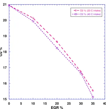
Other effects of EGR include the reduction of intake oxygen concentration. At 0% EGR, the exhaust contains about 11.5% oxygen. With the introduction of EGR, exhaust with lower oxygen concentration replaces the air which has 20.94% oxygen. Thus introduction of EGR reduces the overall oxygen concentration in the intake. Table 4.4 and Figure 4.2 compare the oxygen concentration in the intake at EGR levels ranging between 0 and 35%. As the EGR increased, the intake oxygen concentration reduced almost linearly. Also, when the intake temperature was increased to 40 °C, the intake oxygen concentration reduced at same EGR level. Relatively more intake air was replaced with EGR with the increase in intake temperature leading to a reduction in overall oxygen concentration.

Table 4.4 Variation of intake O2 concentration with EGR % at intake temperature

23°C and 40° C

EGR % O2 % (23 °C Intake) O2 % (40 °C Intake)

0 20.94 20.94

10 20.14 19.94

20 18.64 18.24

30 16.74 16.64

(50)

15 16 17 18 19 20 21 0 5 10 15 20 25 30 35 40 O2 % (23 C intake) O2 % (40 C intake) O 2 % EGR %

Figure 4.2 Comparison of intake O2 concentration for different EGR levels at intake temperatures of 23 °C and 40 °C

4.4 PSO Optimization

The PSO algorithm used in this study was designed to include any number of engine variables as needed. The lower limits, upper limits, and resolutions were defined in a single file engine.txt. The resolutions were set based on the capabilities of the experimental setup. The following equation was used to round the value of the variable to the nearest possible resolution point in each iteration.

ij kkj lmnop qr_uvws tt_ssx lyzj (4.1)

where Xi is the value of the variable i, LLi is the lower limit of the variable i, resi is the resolution of the variable i.

Random numbers used in this optimization were generated using the MATLAB function sum(100*clock). This function generates the random numbers based on the current

(51)

time and date. The random number generator was tested to ensure that the random numbers generated are uniformly distributed between 0 and 1.

All the necessary data that need to be passed on to the next iteration were saved into three files: pnew.txt, pbest.txt, and gbest.txt. Files that are passed on to the next iteration were inserted with iteration number in the file name for easy tracking.

Depending on the number of engine variables and the type of problem, the optimization process can take several days to produce a solution. The program was designed to facilitate the cessation of optimization after any iteration and resumption at a later time.

The operating conditions generated by the program were saved into the file rundatai.txt where ‘i’ is the iteration number. The merit function which will be defined in the next section includes NOx, HC, CO, PM, and BSFC. The NOx, HC, CO, PM, and BSFC data that were collected from the experiments were saved into the file resulti.txt. The program then calculates the fitness function values of each of these experiments to determine the operating conditions of next iteration.