OpenFOAM Simulation for
Electromagnetic Problems
Zhe Huang
Master of Science Thesis in Electric Power Engineering
Department of Energy and EnvironmentDivision of Electric Power Engineering
CHALMERS UNIVERSITY OF TECHNOLOGY Göteborg, Sweden, 2010
September, 2010
Department of Energy and Environment Chalmers University of Technology SE-412 96 Gothenburg
Sweden
Telephone + 46 (0)31-772 1000
Cover:
[Simulation results from ANSYS software]
[Chalmers Reproservice] Gothenburg, Sweden 2010
OpenFOAM Simulation for Electromagnetic Problems Zhe Huang
Department of Energy and Environment Chalmers University of Technology
SUMMARY
Simulation is considered as one of the most important and cost efficient approach of industry research and development. OpenFOAM is one simulation tool with manual solver compilation ability and 3D calculation capability, used for instance for computational fluid dynamics (CFD) [1].
This thesis work is based on the OpenFOAM ‘rodFoamcase’ and the ‘rodFoam’ solver used for plasma arc welding simulations which calculates the magnetic field in air. The thesis work extends the case and the solver to solve electromagnetic field problems for more materials including copper, linear steel and permanent magnets with different geometries. In the future, this work can be applied into the design procedures of electromagnetic devices, like electrical machines.
Based on the Maxwell equations, two different formulations (the A-V formulation and the A-J formulation) are derived to solve magnetrostatic field problems. Formulations are compiled manually into OpenFOAM solvers according to mathematic models by specific program codes. Furthermore, force calculation equations are derived with the Lorenz Force Method and the Maxwell Stress Tensor method. Then, simple geometries with specific initial values and boundary conditions are calculated to test the new solvers. The results of the developed simulation procedures in OpenFOAM are compared to the results of another simulation software; COMSOL Multiphysics. It is found that the simulation results show a very good agreement between OpenFOAM simulations and COMSOL simulations.
Prediction of the future utilization of this thesis work and directions of development are also discussed.
Contents
Symbols and Abbreviations ... 6
1 Introduction ... 7
2 Theoretical Background ... 8
2.1 Maxwell Equations ... 8
2.2 Derived Formulations for 3D Electromagnetic Field Problems ... 8
2.2.1 A-V formulations ... 9
2.2.2 A-J formulations ... 10
2.2.3 Equations for Magnetostatic Field Problems with Permanent Magnets... 10
2.2.4 Transient State Formulations for Electromagnetic Field Problem ... 10
2.3 Formulations for Force Calculations of 3D Problems ... 11
2.3.1 Lorenz Force Method ... 11
2.3.2 Maxwell Stress Tensor ... 11
2.4 Brief Overview of OpenFOAM ... 12
2.4.1 Competitive Strength of OpenFOAM ... 12
2.4.2 File Structure of OpenFOAM Cases ... 13
2.4.3 Solvers Compilation ... 14
3 Implementation in OpenFOAM ... 16
3.1 Modelling Methods ... 16
3.2 Electromagnetic Field Calculation for a Single Bar Geometry ... 16
3.2.1 A-V Solver and A-J solver Comparison on a 3D Geometry ... 16
3.2.2 Comparison between OpenFOAM and COMSOL Simulations on a 2D Axis Symmetric Geometry ... 21
3.3 Single Bar with Copper Ring Geometry ... 24
3.3.1 Geometry Properties ... 24
3.3.2 Mesh Generation ... 24
3.3.3 Boundary Conditions and Initial Values ... 25
3.3.4 Solver Compilation ... 27
3.4 Single Bar with Copper Ring and Permanent Magnets Geometry ... 28
3.4.1 Geometry Properties and Mesh Generation ... 28
3.4.2 Boundary Condition and Initial Values ... 29
3.4.3 Solver Compilation ... 29
3.5 Force Calculation for Two Parallel Current-Carrying Bars ... 30
3.5.1 Geometry Properties ... 30
3.5.2 Boundary Conditions and Initial Values ... 31
3.5.3 Lorenz Force Solver Compilation ... 31
3.5.4 Maxwell Stress Tensor Solver ... 32
4 Results and Discussion ... 33
4.1 Electromagnetic Field of the Single Bar Geometry ... 33
4.1.1 Results from 3D Calculation by the A-V Solver in OpenFOAM ... 33
4.1.2 Results from 3D Calculation by the A-J Solver in OpenFOAM ... 33
4.1.3 OpenFOAM and COMSOL Simulation Comparisons on a 2D Axis ... 34
4.2 Simulation Results of Single Bar with Copper Ring Geometry ... 37
4.3 Simulation Results of the Single Bar with a Copper Ring and Permanent Magnets ... 37
4.4 Simulation Results Comparison of Force Calculation ... 39
4.4.1 Field Distribution Comparison between OpenFOAM and COMSOL ... 39
4.4.2 Numerical Results of Lorenz Force Method and Maxwell Stress Tensor ... 40
Method ... 40
5 Conclusions and Future Work ... 42
Appendix 1 ... 44
Appendix 2 ... 48
Appendix 3 ... 50
Appendix 4 ... 52
Appendix 5 ... 53
References ... 54
Symbols and Abbreviations
⋅ ∇ divergence operator × ∇ curl operator ∇ gradient operator t ∂ ∂ partial derivativeA magnetic vector potential V⋅s/m
B magnetic flux density T
D electric displacement field C/m2
E electric field intensity V/m
H magnetic field intensity A/m
C
H coercive magnetic field of permanent magnets A/m
I current of conductor A
J current density 2
/m A
L total length of conductor m
R resistance Ω
S total area of conductor 2
m
V electrical scalar potential V
ρ electric charge density 3
/m C ε permittivity F/m µ magnetic permeability W A m b/ ⋅ r
µ relative magnetic permeability 0
µ permeability in the free space
ν
magnetic reluctivityr
ν relative magnetic reluctivity
1 Introduction
Since ‘Energy Shortage’ and ‘Greenhouse Effect’ are two of the most severe problems nowadays, energy efficiency and clean energy are becoming more and more important. Further, simulation is considered as one of the most important and cost efficient approach of industry research and development. OpenFOAM is one simulation tool with manual solver compilation ability and 3D calculation capability, used for instance for computational fluid dynamics (CFD) [1].
This thesis work aims at expanding the calculation range of OpenFOAM, by using C++ syntax in OpenFOAM, in order to solve electromagnetic field problems, which can be applied into the design procedures of electromagnetic devices, like electrical machines. The work is one part of electromagnetic devices design performed by the vehicle company Volvo, and will be one step towards reaching the goal of the highest electrical efficiency in electrical machines.
In order to design the optimized geometry and predict the operation behaviour, an accurate knowledge of the field quantities inside the magnetic circuit is necessary [2]. OpenFOAM is a powerful calculation tools for obtaining complex PDE solutions. It has its own superiority compared to other commercial software, which is not only on its free-of-charge and open source licence, but also on its numerous solvers, utilities and libraries [1]. Compared to the ‘black-box’ solvers in other commercial softwares, new physics-mathematics models can be compiled into new solvers based on these features of OpenFOAM.
With implemented methods of the finite element method (FEM), the finite volume method (FVM) and the finite area method (FAM), OpenFOAM is the majority investigated simulation software of this thesis work aimed to enlarge the calculation range to calculate electromagnetic fields. Meanwhile, some of the OpenFOAM cases are simulated in another commercial software COMSOL with the same initial field values and boundary settings. This is done in order to check the validity of the edited solvers with different mathematic models in the OpenFOAM simulations.
These new solvers can be applied into any electromagnetic devices such as an electrical machine, in order to obtain the lowest cost and optimal design.
Chapter 2 describes different ways of formulating static electromagnetic field problems according to Maxwell Equations. Based on the obtained electromagnetic field, two electromagnetic force calculation methods are discussed. Besides, the structure of OpenFOAM files is briefly illustrated.
Chapter 3 gives four practical examples of electromagnetic field and force calculations by OpenFOAM. Each calculation contains the solver compilation and pre-processing, which includes mesh generation, initial values and boundary condition application, and post-processing.
Chapter 4 shows the results of all applications in chapter 3 and also discusses pros and cons of OpenFOAM calculations.
Chapter 5 summarises the thesis work and predicts its future utilizations. Meanwhile other interesting research trends about this topic are also discussed.
2 Theoretical Background
2.1 Maxwell Equations
The complete set of Maxwell equations is shown as below: t D J H ∂ ∂ + = × ∇ (2.1) 0 = ⋅ ∇ B (2.2) t B E ∂ ∂ − = × ∇ (2.3) ρ = ⋅ ∇ D (2.4) where H is the magnetic field intensity, J is the current density, D is the electric flux density, B is the magnetic flux density, t is the time, E is the electric field intensity, andρ is the electric charge density. There is interdependency between all variables in the equations and, therefore, a unique solution [3].
For stationary or quasi-stationary electromagnetic field distribution cases, the displacement current density term
t D ∂ ∂
is neglected, which gives the equation as below
J H = ×
∇ (2.5) Since the divergence of the curl of any vector field in three dimensions is equal to
zero, the following equation is obtained 0 ) (∇× = ⋅ ∇ = ⋅ ∇ J H (2.6) The macroscopic material properties are defined by the constitutive relations [3]:
E D=ε (2.7) H H B=
µ
=µ
rµ
0 (2.8) E J =σ (2.9) whereε
is the permittivity, µ is the magnetic permeability, µr is the relativepermeability, µ0 is the permeability in free space and σ is the electrical conductivity.
2.2 Derived Formulations for 3D Electromagnetic Field
Problems
There are several possible formulations used for electromagnetic field calculations. This thesis work, which focuses on magnetostatic calculations of three-dimensional field problems, are based on the magnetic vector potential A which is defined by
B A= ×
2.2.1 A-V formulations
One type of the magnetic vector potential formulations is the A-V formulation based on magnetic vector potential A coupled with the reduced electric scalar potential V. V is defined in equation (2.11):
V t A E −∇ ∂ ∂ − = (2.11) According to (2.10), the magnetic flux density B can be calculated if the magnetic vector potential A is known. A is defined in the whole problem region. While for the electric scalar potential V, at the two ends of conductor region, a high value of V and a low value of V are defined separately. Also at the non-conducting region, the value of V is zero. Further, the permeability is assumed constant in each material, thus non-linearity of for instance electrical machine core parts are not considered.
For magnetostatic cases, the displacement magnetic vector potential term t A ∂ ∂
is neglected, which gives equation (2.12):
V
E=−∇ (2.12) Combining (2.5) and (2.8) and (2.9) and (2.10) and (2.11), we will get
) ( ) ( 1 ) ( V E J A B H −∇ = = = × ∇ × ∇ = × ∇ = × ∇ σ σ µ µ (2.13)
which is equal to the equation V A =− ∇ × ∇ × ∇ σ µ ( ) 1 (2.14) By using the Coulomb Gauge [4],
0 = ⋅
∇ A (2.15) the A-V formulation in the static case will get the unique solution of A obtained as
below 0 1 1 = ∇ + ⋅ ∇ ∇ − × ∇ × ∇ A A σ V µ µ (2.16) where the second term is a penalty term with the Coulomb gage. Due to the addition of the Coulomb gauge, the solenoidality of the flux density must be satisfied separately [4]. This is done by combining equations (2.6), (2.9) and (2.12) into
∇⋅(−σ∇V)=0 (2.17) Equations (2.16) and (2.17) are compiled into an OpenFOAM solver and is applied for the current-carrying single bar case, which will be further discussed in chapter 3.
2.2.2 A-J formulations
Another type of formula used for static magnetic field calculations is the A-J formulation which uses the electric current density J as driving force.
Combining (2.5) and (2.8) and (2.10), we will get J A B H =∇× = ∇× ∇× = × ∇ ( ) 1 ( ) µ µ (2.18) Using the Coulomb Gauge similar to (2.16), the A-J equation is descripted as
J A A = ⋅ ∇ ∇ − × ∇ × ∇ µ µ 1 1 (2.19) Compared to the A-V formulation, the A-J formulation does not have σ∇V terms, which means it is more time-saving when applying FEM or FVM in the calculation softwares.
2.2.3 Equations for Magnetostatic Field Problems with Permanent Magnets
When different types of magnetic materials are utilized as driving source, the magnetostatic equations below can be applied to calculate the electromagnetic fields, whereHC is the coercive magnetic field of permanent magnets.
1 1 −∇× =0 ⋅ ∇ ∇ − × ∇ × ∇ A A HC µ µ (2.20)[5] This equation can be considered as a transition to equation (2.21) which will calculate the fields generated by two driving sources including electric and magnetic energy sources. J H A A −∇× C = ⋅ ∇ ∇ − × ∇ × ∇ µ µ 1 1 (2.21)
2.2.4 Transient State Formulations for Electromagnetic Field Problem
Because of the time limitation of thesis work, transient equations of field calculation are not used in this report. However, equation (2.22) shows the method to calculate fields for transient electromagnetic problems, which can be helpful for the continuing study.
0 1 1 = ∇ + ∂ ∂ + × ∇ − ⋅ ∇ ∇ − × ∇ × ∇ V t A H A A C σ σ µ µ (2.22)[5]
As it is discussed before, due to the Coulomb Gauge [4] eqation (2.15), the solenoidality of the flux density must be satisfied separately. If formulas (2.6), (2.9) and (2.11) are combined, equation (2.23) will be obtained.
0 = ∇ − ∂ ∂ ⋅ ∇ V t A σ σ (2.23)
2.3 Formulations for Force Calculations of 3D Problems
From the solution of an electromagnetic field problem, the potential or field flux values are calculated firstly. Furthermore, other important parameters, such as force or torque acting on various parts of machines can be obtained from the calculated potential values. Four force or torque calculation methods are mostly used in finite element analysis [6]:
(1) Lorenz Force Method
(2) Maxwell Stress Tensor Method (3) Virtual Work Method
(4) Equivalent Source method
In this thesis work, the Lorenz Force method and the Maxwell Stress Tensor method formulas have been investigated and applied into OpenFOAM in order to calculate electromagnetic force, which are discussed in the following parts.
2.3.1 Lorenz Force Method
The Lorenz Force method can calculate the total force on a current-carrying conductor by volume integration of the force density acting on each differential current-carrying element. The Lorenz force can be calculated by
dV B J
F =∫V( × ) (2.24) where J×Bis the force density of the conductor.
By this method, the total current density J is necessary for the force calculation, which means that this method is relatively easy to get numerical results of coil forces of electrical machines. In contrast, it cannot determine the force acting on ferromagnetic materials [7].
2.3.2 Maxwell Stress Tensor
The Maxwell Stress Tensor method can calculate force acting on a body by integrating force density over a surface enclosing the body. The expression of the Maxwell Stress Tensor is [6]:
) 2 1 ( 1 2 ij j i ij BB B T δ µ − = (2.25)
where i and j can be replaced by (x, y, z) , δij =1 when i=j and δij =0 when i≠j. Therefore the Maxwell Stress Tensor can be expressed in another way as (2.26) [6]:
[
]
[
]
[
]
[
]
[
]
[
]
− − − = = 2 2 2 2 2 2 2 1 ) ( 1 1 1 1 2 1 ) ( 1 1 1 1 2 1 ) ( 1 B B B B B B B B B B B B B B B B B B T T T T T T T T T T z y z x z z y y x y z x y x x zz zy zx yz yy yx xz xy xx µ µ µ µ µ µ µ µ µ (2.26) The force calculation formula in terms of the force density vector is given byTdS dS n B n B B F =∫S ⋅ − ) =∫S 2 1 ) ( 1 ( 2 µ µ (2.27)[6] where n is the normal unit vector to the surface under consideration.
Compared to the Lorenz Force method, the Maxwell Stress Tensor method is more accurate, because this surface integral is not affected by the current density distribution within the object but only by the accuracy of calculated magnetic field density [7]. And this method can be applied to calculate electromagnetic force not only for current source materials but also for ferromagnetic materials. Besides, the integrating surface does not need to be the physical surface of the object, which can be arbitrarily chosen but must be entirely placed in air. Further comparison between the two different force calculation methods is given in chapter 4.
2.4 Brief Overview of OpenFOAM
2.4.1 Competitive Strength of OpenFOAM
OpenFOAM is a C++ based toolbox with revisable solvers to calculate partial differential equations (PDE) and to simulate multi-physics problems, including computational fluid dynamics (CFD). OpenFOAM includes a standard library and great range of solvers, which shows as below [8]:
• Basic CFD
• Incompressible flows • Compressible flows • Multiphase flows
• Direct numerical simulations (DNS) and large eddy simulations (LES) • Combustion
• Heat transfer and buoyancy-driven flows • Particle-tracking flows
• Molecular dynamics
• Direct simulation Monte Carlo • Electromagnetics
• Stress analysis of solids • Finance
This thesis work is focused on extending the ‘Electromagnetics’ solver by using C++ syntax in OpenFOAM.
In order to accomplish one simulation, two branches of files are needed in OpenFOAM. One branch of files which is called ‘case file’ is used to illustrate specific pre-processing, such as geometry, boundary conditions, initiate fields setting and calculation steps and time and so on. The other branch of files which is called ‘solver file’ includes the mathematic model and solution of a certain physic or chemical or economic problem. In 2.4.2, the structures of OpenFOAM cases are shortly introduced. In 2.4.3, the easy and quick equation editing method of OpenFOAM is further described.
Besides, OpenFOAM is also supplied with mesh generator tools, such as blockMesh, extrudeMesh, etc. Meanwhile, it accepts meshes generated by any of the major mesh generators and CAD systems such as ANSYS mesh, CFX 4 mesh, Fluent mesh, etc.
Furthermore, paraFoam, a reader module for OpenFOAM data for the open source visualization application ParaView makes the post-processing of OpenFOAM convenient and user-friendly.
Another reason of simulating in OpenFOAM is its availability of parallel computing, which shows the great potential and opportunity for solving increasingly complex problems.
2.4.2 File Structure of OpenFOAM Cases
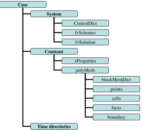
The basic directory structure of an OpenFOAM case, which contains the minimum set of files required to run an application, is shown in figure 2.1 [8]:
Figure 2.1 Directory structure of an OpenFOAM case Case System Constant ControlDict fvSchemes fvSolution xProperties Time directories polyMesh blockMeshDict points cells faces boundary
A ‘system’ directory defines simulation time and calculation algorithms. Meanwhile, it can be used to define different inner fields by using specific utilities, such as ‘setFieldDict’ and ‘funkySetFieldDict’. ‘funkySetFieldDict’ utility is explained in chapter 3 when it is applied into simulation.
A ‘constant’ directory is used to describe the geometry and mesh case in the subdirectory ‘polyMesh’, and specific physical properties (‘xProperties’) for a certain case.
The ‘time’ directories contain different data files of particular fields for a case. Different subdirectories with the name of numbers, which stands for different calculation time steps are included. The ‘0’ directory contains the data files of initialized field values.
The specific functions of each file will be illustrated more detailed in chapter 3. 2.4.3 Solvers Compilation
While OpenFOAM can be used as a standard simulation package, it is also possible to look deep into the ‘black box’ to edit or program different partial differential equations (PDE) by using the finite volume method (FVM) or the finite element method (FEM) or the finite area method (FAM).
As other C++ programming codes, every piece of the original code in the OpenFOAM solvers has to be organised by a standard structure in order to access dependent components of the OpenFOAM library. The top level source file with the .C extension, together with other source files, can be compiled by using the command ‘wmake’, which is included in the directory ‘Make/files’. Figure 2.2 shows the basic directory structure of an OpenFOAM solver [8]:
Figure 2.2 Directory structure of an OpenFOAM solver
In OpenFOAM, there is a top-level code which is applied in the .C file and can represent PDEs directly and flexibly.
For example, if the governing equation is given as equation (2.11): V t A E −∇ ∂ ∂ − = (2.11)
OpenFOAM will represent this equation in its natural language:
solve ( E = = -fvm::ddt(A)-fvm::div(V)) newSolver newSolver.C otherHeader.H Make files options
where fvm stands for Finite Volume Method and returns an fvMatrix, fvc stands for Finite Volume Calculus and returns a geometricField.
Table 2.1 shows some of the correspondence between the mathematic expression and the OpenFOAM expression [8]:
Table 2.1 Correspondence between mathematic expression and OpenFOAM expression [8]
Term description
Mathematical expression fvm::/fvc:: functions
Laplacian ∇⋅Γ∇φ laplacian(Gamma,phi)
φ 2
∇ laplacian(phi)
Time derivative ∂φ/∂t ddt(phi)
Gradient ∇φ grad(phi)
Divergence ∇⋅(ϕ) div(psi)
Curl ∇×φ curl(phi)
The application of these clear structures of ‘case’ and ‘solver’ is further discussed in chapter 3.
3. Implementation in OpenFOAM
3.1 Modelling Methods
With the implemented methods of the finite element method (FEM), the finite volume method (FVM) and the finite area method (FAM), OpenFOAM is the majority investigated simulation software of this thesis work used to calculate electromagnetic fields. Meanwhile, some of the OpenFOAM cases are simulated in another commercial software; COMSOL with the same initial field values and boundary settings, in order to check the validity of the edited OpenFOAM solvers. This thesis work is based on the OpenFOAM ‘rodFoamcase’ and the ‘rodFoam’ solver used for plasma arc welding simulations which calculates the magnetic field in air. The thesis work extends the case and the solver to solve the electromagnetic field problems for more materials including copper, linear steel and permanent magnets with different geometries.
3.2 Electromagnetic Field Calculation for a Single Bar
Geometry
Simulation results from problems with the same 3D geometry and initial values are compared of both A-V and A-J solvers. Another comparison is taken between OpenFOAM and COMSOL on the 2D axis symmetric geometry in order to check the calculation accuracy of the new OpenFOAM solvers. The problem used for the comparisons consists of a single copper bar, surrounded by air, as described further below.
3.2.1 A-V Solver and A-J solver Comparison on a 3D Geometry
(1)Geometry Properties
The problem is defined as follows: Solution domain:
The calculated domain is a cuboid copper wire surrounded by a cuboid air box in 3 dimensions. The geometry data in 3D is given in table 3.1 and figure 3.1 shows the problem region. For the SingleBarCase3D1, high voltage and low voltage are applied to the two ends of the copper bar separately. For the SingleBarCase3D2, current density J is applied to the copper bar. Magnetic fields are calculated for both cases.
Table 3.1 Dimension of single bar geometry
x(m) y(m) z(m)
Conductor 0.4 0,4 6
Figure 3.1 Geometry of the single bar case
Solver name:
SingleBarFoam1 (with A-V solver)
SingleBarFoam2 (with A-J solver) Case name:
SingleBarCase3D1 (with A-V solver)
SingleBarCase3D2 (with A-J solver) (2) Mesh Generation
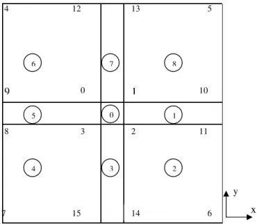
Figure 3.2 shows patches and points defined on the x-y plane (when z=0). Numbers without circles represent different points and numbers with circles represent different patches. The number 0 patch in the middle of the surface represents the cuboid current-carrying cable.
6 7 2 3 8 11 9 0 1 10 5 4 12 13 14 15 1 2 3 4 5 6 7 8 0 z x y
Figure 3.2 Patches and points defined on the x-y plane (z=0) x y left left right front back up down
Generally, there are four validity constraints used in OpenFOAM: points, faces, cells and boundary faces. These are basic constraints that a mesh must satisfy. As it is shown in the figure 3.2, 16 points and 9 faces are defined for the front surface on the x-y plane (z=0). For the whole 3 dimensional geometry, the length along the z- direction is 6 m. Furthermore, the whole length along the z direction is divided into 10 units.
The OpenFOAM ‘BlockMesh’ utility is used to generate meshes in the file
constant /polyMesh/ blockMeshDict of the ‘case’directory.Inside this file, cell shape and mesh density can be defined. Hexahedral, wedge, pyramid, tetrahedron, and tetrahedral wedge cell shapes can be defined by ordering of point labels in accordance with the numbering scheme contained in the shape model. Hexahedral cell shape is used in this thesis work. One example of geometry definition is given in the codes below [8]:
8 //declare the total number of points ( (0 0 0) //point 0 (1 0 0) //point 1 (1 1 0) //point 2 (0 1 0) //point 3 (0 0 0.5) //point 4 (1 0 0.5) //point 5 (1 1 0.5) //point 6 (0 1 0.5) //point 7
A hexahedral block with 10×10×10 mesh density in OpenFOAM is written as:
hex (0 1 2 3 4 5 6 7) (10 10 10) simpleGrading (1 1 1)
The same geometry definition approach is applied to obtain more complex geometry in this thesis work. The comprehensive mesh generation codes of this geometry are given in Appendix 1, which has 400 cells in total.
Besides, the file boundary in the constant /polyMesh directory is used to define type and total number of cells for each patch.
(3) Boundary Condition and Initial Fields for the 3D Geometry Cases
Boundary types are defined in the OpenFOAM file constant /polyMesh /boundary. There are three attributes associated with a patch; the basic type, the primitive type and the derived type. The ‘basic type’ is the one that has been used most often in this thesis work and the different types of basic patches are shown in table 3.2:
Table 3.2 Basic patch types in OpenFOAM
Name Description
Patch generic patch
symmetryPlane plane of symmetry
Empty front and back planes of a 2D geometry
Wedge wedge front and back for an axi-symmmetric geometry
Cyclic cyclic plane
Wall wall—used for wall functions in turbulent flows
For the 3D single bar problem,, ‘patch’ is used for every boundary. The boundary type ‘wedge’ and ‘empty’ are used for the 2D axis symmetric cases later on. One example of ‘boundary’ file is given in Appendix 2.
Field initial values of the boundaries are defined in the so called ‘0’ directory. For the cases using the A-V formulation, the magnetic vector potential A, the electrical scalar potential V and the electrical conductivity σ are pre-defined in the ‘0’ directory. Consequently, for the cases using the A-J formulation, the magnetic vector potential A and the current density J are pre-defined in the ‘0’ directory. The field initial values which need to apply in the inner region of geometries, such as electrical conductivity σ in the cases which use the A-V solver and current density J
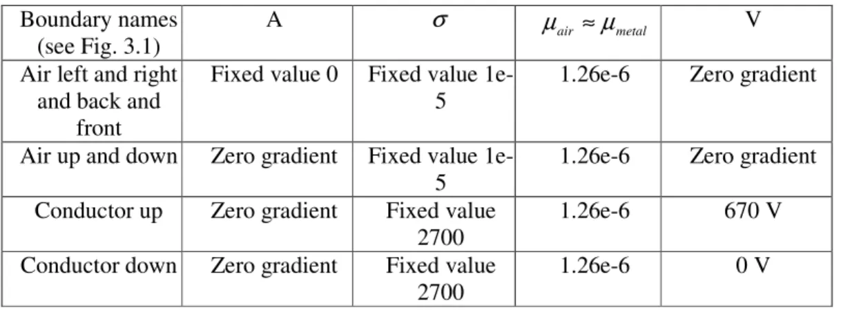
in the cases which use the A-J solver cases, are defined in file system/setFieldDict. Table 3.3 shows the boundary conditions and initial values of the single bar 3D problem when using the A-V formulation. The naming of boundaries are shown in Fig. 3.1.
Table 3.3 Boundary conditions and initial values of the Single Bar 3D problem when using the A-V
formulation Boundary names
(see Fig. 3.1)
A σ µair ≈µmetal V Air left and right
and back and front
Fixed value 0 Fixed value 1e-5
1.26e-6 Zero gradient
Air up and down Zero gradient Fixed value 1e-5
1.26e-6 Zero gradient Conductor up Zero gradient Fixed value
2700
1.26e-6 670 V
Conductor down Zero gradient Fixed value 2700
1.26e-6 0 V
Regarding figure 3.1, the left, right, back and front patches of the air box should be infinitely far from the cable where the magnetic vector potential A is set to 0. The boundary condition “zero gradient” represents that the normal gradient of the field is zero. Since the values of the electrical conductivity are almost zero in air but quite large in metal, 1e-5 S/m is chosen to represent air and 2700 S/m for the metallic material. Furthermore, since the magnetic permeability µ of air in some cases is almost equal to the value of metal, such as copper, 1.26e-6 Wb/A⋅m is chosen in this simulation.
In order to have the same driving force with the A-J formulation as it is using the A-V formulation (which applies 670V) a current density of 310500A/m2 is applied, according to the calculation below:
σ σ L J S L I R I U = ⋅ ⋅ ⋅ = ⋅ = i.e. 2 / 301500 6 2700 670 m A L U J = ⋅σ = ⋅ =
where U is the voltage of the conductor, I is the current of the conductor, L is the total length of the conductor, and S is the total area of the conductor.
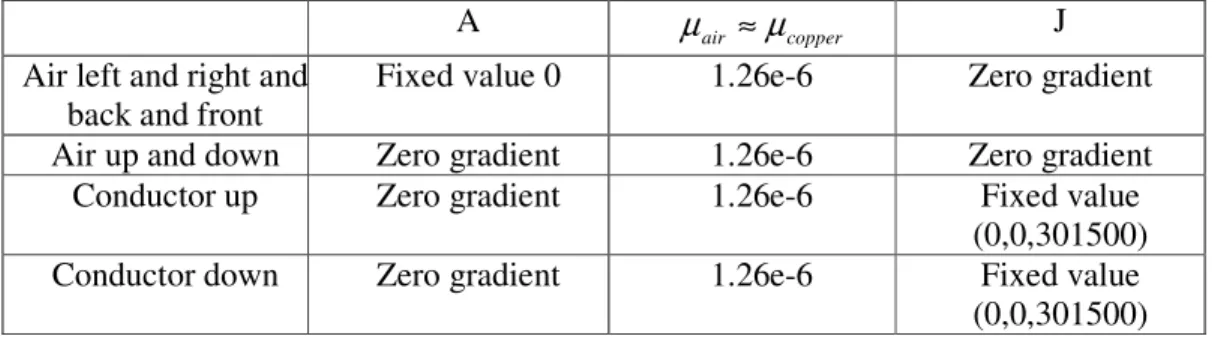
Table 3.4 shows the boundary condition and initial values of the single bar 3D simulation when the A-J formulation is applied.
Table 3.4 Boundary condition and initial values of the single bar 3D problem when using the A-J formulation
A µair ≈µcopper J Air left and right and
back and front
Fixed value 0 1.26e-6 Zero gradient
Air up and down Zero gradient 1.26e-6 Zero gradient
Conductor up Zero gradient 1.26e-6 Fixed value
(0,0,301500)
Conductor down Zero gradient 1.26e-6 Fixed value
(0,0,301500) Appendix 3 gives an example of an initial field setting file ‘A’ in the ‘0’ directory. Further, Appendix 4 shows the inner field setting method of the current density J.
(4)Solver Compilation and Calculation
As it is shown in chapter 2, the A-V formulation in the magneto static case is given as in (2.16) and (2.17) where (2.16) is repeated below:
0 1 1 = ∇ + ⋅ ∇ ∇ − × ∇ × ∇ A A σ V µ µ (2.16) The A-J formulation in the magneto static case is given as the following:
J A A = ⋅ ∇ ∇ − × ∇ × ∇ µ µ 1 1 (2.19) Since
(
∇×F)
=∇(
∇⋅F)
−∇2F × ∇ (3.1) the A-V formulation and the A-J formulation can be transformed into formula (3.2) and (3.3):0 1 2 = ∇ + ∇ − A σ V µ (3.2) J A= ∇ − 1 2 µ (3.3) Together with equation (2.17), these partial differential equations can be expressed by the following OpenFOAM codes:
(a) A-V Solver equations
solve ( fvm::laplacian(sigma, ElPot) );
solve ( fvm::laplacian(A)==sigma*muMag*(fvc::grad(ElPot)) ); B= fvc::curl(A);
Je=-sigma*(fvc::grad(ElPot));
(b)A-J Solver equations
solve ( fvm::laplacian(A)==-muMag*J); B= fvc::curl(A);
where muMagis the permeability (of air and the copper conductor).
Appendix 5 gives an example of the .C file of the A-J solver. This .C file combined with the files in the ‘Make’ directory (refer to figure 2.2) can be compiled by the ‘wmake’ command. After compilation, an executable file of the new solver is generated. The executable file should be copied into the ‘Case’ directory and it is used for calculations with specific boundary conditions and initial values.
(5)Post-processing
Post-processing is executed by the command ‘paraFoam’ which will call the ‘paraView’ software which is the main post-processor of OpenFOAM. After calculation, the maximum value of current density, magnetic vector potential and magnetic field density are compared between the A-V solver and the A-J solver which is further discussed in chapter 4.1.
3.2.2 Comparison between OpenFOAM and COMSOL Simulations on a 2D Axis Symmetric Geometry
Chapter 4.1 will show great similarity of calculation results from the OpenFOAM A-V solver and A-J solvers applied to the same 3D geometry. Hence, if OpenFOAM calculation results from the A-V solver show similarity to COMSOL calculation results from this simulation test, the validity of the A-J solver in the 2D axis-symmetric case should also be proved.
OpenFOAM needs 3D control volumes even for the 2D cases. However, the patch type ‘empty’ can be applied to generate 2D or even 1D geometries by specifying special patches into empty in one dimension or in two dimensions. Meanwhile, the patch type ‘wedge’ can be used to specify a geometry as a wedge with a small angle and being one cell thick along the plane of symmetry to obtain a 2D axi-symmetric geometry, which is applied in the simulation below.
(1) Geometry properties for 2D axi-symmetric simulation applied in OpenFOAM and COMSOL
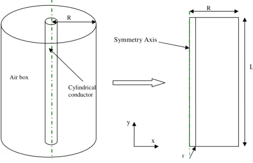
2D axi-symmetric simulations are done both in OpenFOAM and COMSOL to calculate electromagnetic fields of a cylindrical conductor placed in a cylindrical air box. The 2D axi-symmetric geometry is shown in the right figure of figure 3.3 and the geometry data is shown in table 3.5, where R is the radius of the cylindrical air box, r is the radius of the cylindrical conductor, and L is the total length of the geometry.
Figure 3.3 Geometry from 3D to 2D axis symmetric
Table 3.5 Data of 2D axis symmetric geometry r(inner)(m) R(outer)(m) L(m) 0.2 2 6 x L R y r Symmetry Axis R Air box Cylindrical conductor
(2) Mesh Generation
In OpenFOAM, the square meshes are still applied in the 2D axis symmetric geometry; 10 cells are applied on the x direction and 30 cells are applied on the y direction. Meanwhile, 1 cell unit is applied along the z direction to express the 2D geometry. In COMSOL, the mesh generation is done by the default mesh type ‘Normal’.
(3) Boundary Condition and Initial Field
As shown in table 3.6 and table 3.7, the current density is used as the driving force in COMSOL and the equivalent voltage is applied for the A-V solver in OpenFOAM. In COMSOL, the current density is set to 0.3A/mm2along y direction. Consequently, in OpenFOAM, a voltage value of 670V is applied to the cylindrical conductor, in order to introduce a current density of 0.3A/mm2.
Table 3.6 Initial values for single bar simulation with 2D axis symmetric geometry in COMSOL µ(H/m) J ( / 2
mm
A ) σ (S/m)
copper 1.26e-6 0.3 2700
air 1.26e-6 0 1e-5
Table 3.7 Initial values for single bar simulation with 2D axis symmetric geometry in OpenFOAM µ(H/m) U(V) σ (S/m)
copper 1.26e-6 High: 670, Low: 0 2700
Air 1.26e-6 0 1e-5
There is one difference between OpenFOAM and COMSOL when they are used for 2D axis symmetric simulation. In COMSOL, when 2D simulation is taken, 2D geometry is drawn at the first place. In OpenFOAM, though 2D simulation is needed to be done, 3D geometry is always needed to be drawn first. Then 2D axis
symmetric simulation is needed, the boundary conditions of two surfaces which are parallel to the rotating axis are treated as type ‘wedge’. Table 3.8 shows the
boundary conditions applied in this single bar 2D axis symmetric simulation. Table 3.8 Boundary conditions for single bar simulation with 2D axis symmetric geometry in
OpenFOAM
A(V⋅s/m) U(V)
Air up and down and back and front
Fixed value 0 Zero gradient
Air left and right Wedge Wedge
Copper bar up Zero gradient Fixed value 670 Copper bar down Zero gradient Fixed value 0
3.3 Single Bar with Copper Ring
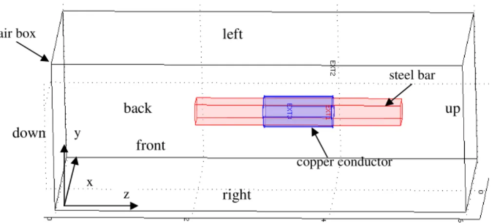
In this simulation, three different materials; a copper ring conductor, a steel bar and air, are involved. As it is shown in figure 3.4 below, the cuboid steel bar is put in the middle of the copper ring conductor.
Figure 3.4 Geometry of a steel cuboid bar with a ring-shape copper conductor
3.3.1 Geometry Properties
The geometry data of a steel cuboid bar with a ring-shape copper conductor is shown as the table 3.9 below.
Table 3.9 Geometry data table of single bar with copper ring case
x(m) y(m) z(m) Air Box 4 4 6 Steel Bar 0.14 0.14 3 Inner R Outer R Z Copper Ring 0.2 0.21 1 3.3.2 Mesh Generation
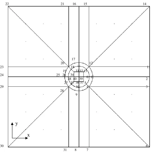
The mesh on x-y plate, for the simulation with one copper conductor and one cuboid steel bar, is generated as it is shown in figure 3.5.
z x y up down front back left right air box steel bar copper conductor
Figure 3.5 Patches and points definition in the x-y plane
As it is shown in figure 3.5 of the ‘up surface’ in the x-y plane, 41 points are defined. For the whole 3D geometry, 82 points and 35 blocks are defined to illustrate the steel bar rounded by the copper tube which is surrounded by air. The mesh definition approach is similar to the approach applied in the single bar case. 3.3.3 Boundary Conditions and Initial Values
The current density, J, in the ring shaped coil (with a magnitude of unity) can be expressed as below:
=
+ + −0
,
,
2 2 2 2 y x x y x yJ
In order to set the coil different permeability values, the ‘funkySetField’ utility is used. Compared to the utilization of the utility setFieldDict used in previous cases, this utility can set non-uniform field values and non-uniform field application regions by C++ commands whereas the utility setFieldDict can only set uniform fields. The OpenFOAM C++ commands used instead of the mathematic expressions to set the fields are given in the text below. The commands are put in the file
system/funkySetFieldsDict. 0 1 2 3 4 5 6 7 8 9 10 11 12 13 15 16 17 18 19 20 21 22 23 25 26 24 27 28 29 30 31 32 33 34 35 36 37 38 40 39 14 x y
currentdensity2 {
field J; //field initialise
expression “vector( -301500*pos().y/sqrt(pow(pos().x,2)+pow(pos().y,2)), 301500*pos().x/sqrt(pow(pos().x,2) +pow(pos().y,2)), 0)”; //ring-shaped current
condition “sqrt(pow(pos().x,2)+pow(pos().y,2))>=0.2 &&
sqrt(pow(pos().x,2)+pow(pos().y,2))<=0.21 && pos().z>=3 && pos().z<=4”; keepPatches 1;
dimensions [0 -2 0 0 0 1 0]; }
In the code above, ‘field’ is used to declare one field, ‘expression’ is used to write field values, ‘condition’ will select a subset of the cells, and ‘dimensions’ describes the dimension of the field in SI units.
In this simulation, the relative permeability is assumed to be constant (thus saturation effects are ignored), and relative reluctivity can be expressed as in formula (3.4), µ µ µ ν ν 1 1 0 0 = ⋅ = ⋅ r r (3.4)
where ν0 is the reluctivity of air, νr is the relative reluctivity of other materials, µ0 is the permeability of air and µris the relative permeability of other materials.
The ‘funkySetField’ utility is used to express different permeabilities for different regions in the following simulations. In the ‘funkySetField’ utility, one parameter, such as permeability (or reluctivity), can be assigned with different values in different volumes by changing the commands ‘expression’ and ‘condition’. The field values are assigned by command ‘expression’, and the regions applying the corresponding field values are declared by command ‘condition’. Besides, the latter applied field value will overlap the previous field value for the same region. Different relative permeabilities (or reluctivities) are defined by the command below in the ‘funkySetFieldDict’ file.
relativereluctivity2 //copper ring {
field viR; //field to initialise
expression “1”; //relative reluctivity in ring
condition “sqrt(pow(pos().x,2)+pow(pos().y,2))>=0.2 &&
sqrt(pow(pos().x,2)+pow(pos().y,2))<=0.21 && pos().z>=3 && pos().z<=4”; keepPatches 1;
dimensions [0 0 0 0 0 0 0]; }
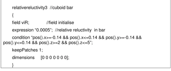
relativereluctivity3 //cuboid bar {
field viR; //field initialise
expression “0.0005”; //relative reluctivity in bar
condition “pos().x>=-0.14 && pos().x<=0.14 && pos().y>=-0.14 && pos().y<=0.14 && pos().z>=2 && pos().z<=5”;
keepPatches 1;
dimensions [0 0 0 0 0 0 0]; }
In order to show the permeability difference between the coil and the steel, a high permeability value (2000) is chosen for the steel bar. Table 3.10.1 and table 3.10.2 show the initial values and boundary conditions after executing funkySetField utility.
Table 3.10.1 Initial values for a copper coil with steel bar geometry: J( / 2 m A )(absolute value) µr(νr) Air 0 1 (1) Coil 301500 1 (1) Steel bar 0 2000 (0.0005 )
Table 3.10.2 Boundary conditions for a copper coil with steel bar geometry:
A(V⋅s/m) J( 2
/m
A )
Air left and right and back and front
Fixed value 0 Zero gradient Air up and down Zero gradient Zero gradient Steel bar up Zero gradient Zero gradient Steel bar down Zero gradient Zero gradient
Since the copper conductor only have inner boundaries in this simulation, there is no outer boundary definition for the conductor.
3.3.4 Solver Compilation
In order to solve the problem, a general solver including permanent magnets materials (which will be contained in the next simulation) is treated, and thus this new solver, JAHcFoam, includes the coercive magnetic field,HC.
According to the equation in section 2.2.3, the following equation (2.21)
J H A A −∇× C = ⋅ ∇ ∇ − × ∇ × ∇ µ µ 1 1 (2.21) can be changed into
C H J A=− −∇× ∇2 1 µ (3.5) In order to simplify the equation expression in OpenFOAM, equation 3.4 is applied.
Then (2.21) can be changed into equation (3.6):
(
⋅ r∇×A)
−∇(
⋅ r∇⋅A)
−∇×HC =J×
∇ ν0 ν ν0 ν (3.6)
Equation (3.6) can be written in OpenFOAM by the following code:
solve ( viMag*viR*fvm::laplacian(A)==-J-fvc::curl(Hc));
Since there are no permanent magnetic materials in this simulation, Hc is set to 0 in the file funkySetFieldDict when applying the new solver.
The simulation results are discussed in chapter 4.
3.4 Single Bar with Copper Ring and Permanent Magnets
Compared to the geometry of the previous problem (the steel bar with the ring coil) the dimensions of the steel bar, ring-coil and the air box are kept. However, a permanent magnet block is inserted as another magnetic field generating source. 3.4.1 Geometry Properties and Mesh GenerationThe geometry data is given in table 3.11 and seen in figure 3.7.
Table 3.11 Geometry data of a single bar and copper ring and a permanent magnet
x(m) y(m) z(m)
Air box 4 4 6
Steel bar 0.14 0.14 3
Permanent magnetic block 0.14 0.14 0.2
Inner R Outer R z
Figure 3.7 Geometry of a single bar with a copper ring and a permanent magnet
The same mesh generation method as in the previous case (which includes a cuboid steel bar and a copper conductor) is applied in this simulation. But the mesh along the z dimension is increased from 10 to 60 in order to obtain accurate enough calculation results for the permanent magnet of which the thickness is 0.2m.
3.4.2 Boundary Condition and Initial Values
Compared to the the previous case (the cuboid steel bar and a copper conductor), the coercive magnetic field value of a permanent magnet is added by the following command.
magnetization4 {
field M; //field initialise
expression “vector(724000,0,0)”; //coercive magnetic field in permanent magnets
condition “pos().x>=-0.14 && pos().x<=0.14 && pos().y>=-0.1 && pos().y<=0.1 && pos().z>=1.3 && pos().z<=1.5”;
keepPatches 1;
dimensions [0 -1 0 0 0 1 0]; }
Since the copper conductor and magnet block only have inner boundaries in this simulation, there is no outer boundary definition for the conductor and magnet block. 3.4.3 Solver Compilation
The new solver based on formulation (3.6) can be applied to calculate electromagnetic field including permanent magnetic materials. Simulation results are discussed in chapter 4. z x y Air box Permenant magnet Steel bar Copper conductor
3.5 Force Calculation for Two Parallel Current-Carrying
Bars
Based on the methodologies of electromagnetic force calculation in chapter 2, formulations of the Lorenz Force Method and the Maxwell Stress Tensor Method are compiled in OpenFOAM. Furthermore, the results calculated from the compiled solvers in OpenFOAM are compared with the results calculated from COMSOL. 3.5.1 Geometry Properties
In this simulation, force is calculated between two current-carrying cuboid bars which are placed in parallel and surrounded by air, see figure 3.8. The distance (in the x-y plane, from centre to centre) between bar1 and bar2 is 0.6m. In order to obtain the infinite long and thin cables, 10m is applied for the length and 0.4m is applied to the width for both cables. Geometry data is given in table 3.13.
Figure 3.8 Geometry of two parallel bars for force calculation
Table 3.13 Geometry data of two parallel bars for force calculation
X(m) Y(m) Z(m) Air box 2 2 10 Bar1 0.4 0,4 10 Bar2 0,4 0,4 10 x z y
3.5.2 Boundary Conditions and Initial Values
In this simulation, 1A and -1A current with opposite directions are applied into the two parallel bars separately. The current densities are calculated using the formula below, where J is the current density, I is the current flowing through one conductor and S is the total area of one conductor.
= = S I J 2 2 6.25 / 4 . 0 4 . 0 1 m A m A = ×
Table 3.14.1 and table 3.14.2 show the initial values and boundary conditions of the force calculation case.
Table 3.14.1 Initial value for force calculation case
J(A/m2) Hc(A/m) µr µ0(N/A2)
Air box (0, 0, 0) 0 1 1.26e-6
Bar 1 (0, 0, 6.25) 0 0.999 994 1.26e-6
Bar 2 (0, 0, -6.25) 0 0.999 994 1.26e-6
Table 3.14.2 Boundary condition for force calculation case
A(V⋅s/m) J( 2
/m
A ) HC( A/m)
Air left and right and back and front
Fixed value 0 Zero gradient Zero gradient Air up and down Zero gradient Zero gradient Zero gradient Left bar up and down Zero gradient Fixed value
(0,0,6.25)
Zero gradient Right bar up and
down
Zero gradient Fixed value (0,0,-6.25)
Zero gradient
3.5.3 Lorenz Force Solver Compilation
One header file Force.H is applied to calculate Lorenz Force by executing volume integration of Lorenz Force density. This header file is called by the major solver file (.C file). The formulation of Lorenz Force calculation in the header file is given as below:
F= Jtot^B
A loop of the volume integration for Lorenz Force density on one of the bars in file Force.H is calculated using the method below, where dz1 is the length of one cell in the z direction.
//--- loop for calculating Lorenz Force in the cross section forAll(mesh.C(), celli)
{
if(C1x[celli]>=-0.7 && C1x[celli]<=-0.3 && C1y[celli]>=-0.2 && C1y[celli]<=0.2) // ---define the volume which will be applied volume integration for
{
F11[celli]=J[celli] ^ B[celli];
//---Lorenz Force density is calculated cell by cell Force11=Force11+F11[celli]*(mesh.V()[celli]);
//---Lorenz Force is obtained by the volume integration of the whole defined volume
} }
3.5.4 Maxwell Stress Tensor Solver
According to equation (2.26), nine components of Maxwell Stress Tensor are expressed in the major solver file (.C file) by the code below.
Txx = 1/muMag*((B.component(0)*B.component(0))-(0.5*(B&B))); Txy= 1/muMag*(B.component(0)*B.component(1)); Txz=1/muMag*(B.component(0)*B.component(2)); Tyx = 1/muMag*(B.component(1)*B.component(0)); Tyy = 1/muMag*((B.component(1)*B.component(1))-(0.5*(B&B))); Tyz = 1/muMag*(B.component(1)*B.component(2)); Tzx = 1/muMag*(B.component(2)*B.component(0)); Tzy = 1/muMag*(B.component(2)*B.component(1)); Tzz = 1/muMag*((B.component(2)*B.component(2))-(0.5*(B&B)));
In order to calculate electromagnetic force from Maxwell Stress Tensor, a surface enclosing the object which the force is acting on is chosen to execute surface integration. Since the force along the z dimension is small enough to be neglected, only the surface integral of four surfaces which are parallel to the z direction around each cuboid bar is treated. One surface integration example is given below:
//---force in the cross section 1
//--- read force density 1 for the whole volume F2[celli]=(T[celli]&vector(1,0,0));
//---surface integral
if((mag(C2x[celli]+0.1)<=0.015) && C2y[celli]>=-0.8 && C2y[celli]<=0.8) {
F2s=F2s+(F2[celli]*(mesh.V()[celli]/0.03)); }
4 Results and Discussion
After the implementation of pre-processing, which includes geometries, meshes, boundary conditions and initial values, processing and calculations are done by applying the corresponding solvers. Later on, post-processing can be executed to get direct viewing results which are illustrated below. Also, the pros and cons of OpenFOAM simulation are discussed.
4.1 Electromagnetic Field of the Single Bar Geometry
In the following sections, 3D simulations are done for ‘a single bar surrounded by air’ geometry in OpenFOAM by applying the A-V solver and the A-J solver separately. Results given by the two different solvers are compared as well.
4.1.1 Results from 3D Calculation by the A-V Solver in OpenFOAM
After 3D calculation by the A-V solver, the maximum values of current density
Je, vector potential A and magnetic flux density B are given in the table 4.1. Figure 4.1 gives the surface plots of the three parameters for the single bar geometry.
Table 4.1 Maximum values from 3D calculation for single bar geometry by A-V solver Je(A/m2) A(V⋅s/m) B(T)
301500 0,0269804 0,0411579
Figure 4.1 Surface plotsfrom 3D calculation for single bar geometry by A-V solver
4.1.2 Results from 3D Calculation by the A-J Solver in OpenFOAM
For this simulation, the current density J is one of the applied initial values, and the calculated fields are vector potential A and magnetic flux density B. The maximum values of A and B are given in table 4.2 and the surface plots of current density, vector potential and magnetic flux density are shown in figure 4.2.
Table 4.2 Maximum values from 3D calculation for single bar geometry by A-J solver A (V ⋅s/m) B (T)
0,0269804 0,0411579
Figure 4.2 Surface plots from 3D calculation for single bar geometry by A-J solver
As seen in the OpenFOAM calculation results above, the maximum values and field distribution of magnetic flux density are the same no matter if voltage or equivalent current density is applied as driving source. In both of the cases, the maximum values of magnetic flux density B are obtained in close proximity to the edge of the conductor.
4.1.3 OpenFOAM and COMSOL Simulation Comparisons on a 2D Axis Symmetric Geometry
Next section shows the simulation results from OpenFOAM and COMSOL about the single bar geometry by the 2D axis symmetric method.
As discussed in chapter 3, the same values of magnetic permeability µ and electrical conductivity σ are applied both in OpenFOAM and COMSOL. Current density is applied in COMSOL and the equivalent voltage as driving source is applied in OpenFOAM.
(a) The maximum field values calculated by both softwares are given in table 4.3 and table 4.4 separately. Figure 4.3 uses bar chart to illustrate the difference of
maximum values between the OpenFOAM calculation and the COMSOL calculation.
Table 4.3 Maximum field values from OpenFOAM
J(A/m2) B (T) A (V⋅s/m)
3.015e5 0.0370033011 0.0224271994
Table 4.4 Maximum field values from COMSOL
J(A/m2) B (T) A (V⋅s/m)
3e5 0.0377 0.0212
Figure 4.3 Comparison of results given by OpenFOAM and COMSOL
As shown in table 4.3 and table 4.4, the results from OpenFOAM and COMSOL show a 5.7% difference in the magnetic vector potential A and 1.8% for the magnetic flux density B. This comparison shows great similarity between the calculations from OpenFOAM and COMSOL.
(b) Figure 4.4 and figure 4.5 show the field distributions of the magnetic vector potential A and magnetic field density B:
Figure 4.4 Surface plots of magnetic vector potential and magnetic field density in OpenFOAM
Figure 4.5 Surface plots of magnetic vector potential and magnetic field density in COMSOL As one can see here, the surface plots on magnetic vector potential A and magnetic field density B from OpenFOAM and COMSOL show great similarity, which can prove the accuracy of OpenFOAM calculation.
(c) Magnetic field distributions obtained from OpenFOAM and COMSOL calculations are further compared by using a line plot approach along a line which is parallel to the x axis and passes through point (0, 3). Figure 4.5 and figure 4.6 show the line plots obtained by the two softwares:
Figure 4.6 Line plot of magnetic flux density B along the x coordinate when y=3 in OpenFOAM (length VS magnetic flux density B)
Figure 4.7 Line plot of magnetic flux density B along the x coordinate when y=3 in COMSOL (length VS magnetic flux density B)
According to the results above, when current density values are around 3e5 A/m2 the maximum value of magnetic flux density B is about 0.37T from both OpenFOAM and COMSOL calculations.
From the distribution plot of flux density B from COMSOL calculation in figure 4.7, the magnetic flux density is increased from zero obtained at x=0m to the maximum value at the rim of the conductor when x=0.2m. Later on, the flux density
B is decreased again from the rim of the conductor (when x=0.2m) to the rim of the air box (when x=2m). This distribution of flux density B also confirms the distribution of B obtained from 3D simulations above.
Comparing the field distribution plot of flux density B from the OpenFOAM calculation in figure 4.6 to figure 4.7, the main distribution trends are the same, but one calculation difference can be observed. In figure 4.6, the magnetic flux density
B is started from a small non-zero value at x=0 and is ended at x=2.25m. The reason to this phenomenon in OpenFOAM can be the unit square mesh application. Thus, the calculation procedure cannot distinguish the starting calculation point within one cell distance. This problem should be solved by applying a finer mesh in the future work.
One problem should be pointed out that, in 2D axis-symmetric geometry, the A-V solver can solve the electromagnetic problems with low electrical conductivity σ values but not the cases with high electrical conductivity. The reason of this problem has not been defined. But since the A-J solver will not involve any electrical conductivityσ, it doesn’t have this issue at all.
4.2 Simulation Results of the Single Bar with Copper Ring
Relative permeability refers to a material’s ability to attract and conduct magnetic lines of flux. The more conductive a material is to magnetic fields, the higher its permeability [9]. As it is shown in the comparison figure 4.8, after setting a high permeability (low reluctivity) in the steel bar in the middle of the ring-shape conductor, the magnetic flux density B is confined to a path which closely couples the ring –shape conductor and more flux density lines go through the more conductive path- the steel bar. The simulation with the same geometry, boundary conditions and initial values is done in COMSOL as well. The results are compared in the left hand side pictures of fig 4.9 and 4.10.Figure 4.8 Line plots comparison between cases with and without high permeability steel bar
4.3 Simulation Results of the Single Bar with a Copper Ring
and Permanent Magnets
As it is discussed in chapter 3.4.2, the initial values and boundary conditions in table 3.11 are applied both in OpenFOAM and COMSOL. A coercive magnetic field
Hc with a value of (72400, 0, 0) is applied to represent permanent magnetic material in both soft-wares. As it is shown in figure 4.9 and 4.10 (the two pictures at the right side), coercive magnetic field Hc is applied along the x axis. The magnetic fields distribution plots for geometries with (the plots at the right side) and without (the plots at the left side) permanent magnetic materials are obtained from COMSOL and OpenFOAM separately. Results are shown in figure 4.9 and figure 4.10.
Line Plot of Magnetic Flux Density B
when Relative Reluctivity=1 in steel bar
Line Plot of Magnetic Flux Density B
when Relative Reluctivity=5e-4 in steel bar
Figure 4.9 Surface plots from COMSOL
Figure 4.10 Surface plots from OpenFOAM
In both surface plots from COMSOL in figure 4.9 and OpenFOAM in figure 4.10, the comparisons between the figures at the left side and the figures at the right side show that, the magnetic flux density B is greatly increased after adding permanent magnetic material.
Furthermore, the comparison between the two plots on the right side in figure 4.9 and figure 4.10 shows better computing ability in OpenFOAM than COMSOL for this 3D simulation case including a permanent magnet. In OpenFOAM, a suitable mesh approach can be decided according to the complexity of one specific geometry. For this simulation done by the author, COMSOL can only solve this problem with ‘coarser’ mesh because of the limitation of computer memory, which gives the worse field distribution stream line as plot of 4.9 (to the right).
x z y x y z
On the other hand, regarding to this simulation in OpenFOAM, there is no inner boundary that can be set for the permanent magnetic block. Meanwhile, the size of the permanent magnet block is defined by setting application areas of coercive magnetic field in funkySetField utility as it is shown in chapter 3. Hereby, the minimum length of each mesh volume on every dimension for a 3D geometry will influence the accuracy of the calculation. For example, the thickness in the z direction of the permanent magnet block is 0.2m in this simulation. If 40 cells are chosen for a 6 m long geometry, the maximum cell length will be 0.15m along z, which can bring large errors into the calculation. In this simulation, 60 cells are applied for the magnet block on the z direction to avoid this mistake.
4.4 Simulation Results Comparison of Force Calculation
Force calculations are applied for two parallel current carrying bars. In order to obtain the infinite long and thin bars, 10m as length and 0.4m as width are applied for both bars. The distance between two bars from centre to centre is 0.6m.
4.4.1 Field Distribution Comparison between OpenFOAM and COMSOL
In figure 4.11, the surface plots of force density distribution calculated from OpenFOAM and COMSOL are compared. For the convenience of the following discussion, the terms ‘inner edge’ and ‘outer edge’ are defined as shown in figure 4.11. Both plots illustrate that the forces acting on the inner edges of two parallel cables are larger than the forces acting on the outer edges. Further the shorter distance between the two bars, the larger the magnetic force is.
Figure 4.11 Surface plots of force density distribution from OpenFOAM and COMSOLcalculations
surface plot of Lorenz Force density in OpenFOAM
surface plot of Lorenz Force density in COMSOL
inner edge
outer
edge left right
![Table 2.1 Correspondence between mathematic expression and OpenFOAM expression [8]](https://thumb-us.123doks.com/thumbv2/123dok_us/1787982.2755262/15.918.177.744.247.491/table-correspondence-mathematic-expression-openfoam-expression.webp)