4–72
Introduction
Applications Where Water Is Appropriate
Water is the most commonly used fire extinguishing agent, mainly due to the fact that it is widely available and inexpensive. It also has very desirable fire extin-guishing characteristics such as a high specific heat and high latent heat of vaporization. A single gallon of water can absorb 9280 Btus (2586.5 kJ) of heat as it increases from a 70ÜF (21ÜC) room temperature to become steam at 212ÜF (100ÜC).
Water is not the perfect extinguishing agent, how-ever, and is considered inappropriate for the protection of certain water reactive materials. In some cases, the use of water can produce heat, flammable or toxic gases, or ex-plosions. The quantities of such products must be con-sidered, however, because application of sufficient water can overcome the reaction of minor amounts of these materials.
Another drawback of water is that it is more dense than most hydrocarbon fuels, and immiscible as well. Therefore, water will not provide an effective cover for burning hydrocarbons, or mix with them and dilute them to the point of not sustaining combustion. Instead, the hy-drocarbons will float on top of the water, continuing to burn and possibly spread. To combat such fires, foam so-lutions can be introduced into the water to provide an ef-fective cover and smother the fire. Applying water in a fine mist has also been successful.
However, even when water from sprinklers will not suppress the fire, its cooling ability can protect structural elements of a building by containing the fire until it can be extinguished by other means.
Types of Sprinkler Systems
Automatic sprinkler systems are considered to be the most effective and economical way to apply water to suppress a fire. There are four basic types of sprinkler systems:
1. Awet pipe system is by far the most common type of sprinkler system. It consists of a network of piping containing water under pressure. Automatic sprinklers are connected to the piping such that each sprinkler protects an assigned building area. The application of heat to any sprinkler will cause that single sprinkler to operate, permitting water to discharge over its area of protection.
2. Adry pipe system is similar to a wet system, except that water is held back from the piping network by a spe-cial dry pipe valve. The valve is kept closed by air or nitrogen pressure maintained in the piping. The oper-ation of one or more sprinklers will allow the air pres-sure to escape, causing operation of the dry valve, which then permits water to flow into the piping to suppress the fire. Dry systems are used where the wa-ter in the piping would be subject to freezing.
3. A deluge system is one that does not use automatic sprinklers, but rather open sprinklers. A special deluge valve holds back the water from the piping, and is ac-tivated by a separate fire detection system. When acti-vated, the deluge valve admits water to the piping network, and water flows simultaneously from all of the open sprinklers. Deluge systems are used for pro-tection against rapidly spreading, high hazard fires. 4. Apreaction system is similar to a deluge system except
that automatic sprinklers are used, and a small air pressure is usually maintained in the piping network to ensure that the system is air tight. As with a deluge system, a separate detection system is used to activate a deluge valve, admitting water to the piping. How-ever, because automatic sprinklers are used, the water is usually stopped from flowing unless heat from the fire has also activated one or more sprinklers. Some
CHAPTER 3
Automatic Sprinkler
System Calculations
Russell P. Fleming
Russell P. Fleming, P.E., is vice president of engineering, National Fire Sprinkler Association, Patterson, New York. Mr. Fleming has served as a member of more than a dozen NFPA technical commit-tees, including the Committee on Automatic Sprinklers. He cur-rently serves on the Board of Directors of NFPA.
special arrangements of preaction systems permit vari-ations on detection system interaction with sprinkler operation. Preaction systems are generally used where there is special concern for accidental discharge of wa-ter, as in valuable computer areas.
These four basic types of systems differ in terms of the most fundamental aspect of how the water is put into the area of the fire. There are many other types of sprin-kler systems, classified according to the hazard they pro-tect (such as residential, in-rack, or exposure propro-tection); additives to the system (such as antifreeze or foam); or special connections to the system (such as multipurpose piping). However, all sprinkler systems can still be cate-gorized as one of the basic four types.
Applicable Standards
NFPA 13, Standard for the Installation of Sprinkler Sys-tems (hereafter referred to as NFPA 13), is a design and in-stallation standard for automatic sprinkler systems, referenced by most building codes in the United States and Canada.1 This standard, in turn, references other
NFPA standards for details as to water supply compo-nents, including NFPA 14, Standard for the Installation of Standpipe and Hose Systems; NFPA 20, Standard for the In-stallation of Centrifugal Fire Pumps (hereafter referred to as NFPA 20); NFPA 22, Standard for Water Tanks for Private Fire Protection (hereafter referred to as NFPA 22); and NFPA 24, Standard for the Installation of Private Fire Service Mains and Their Appurtenances.
For protection of warehouse storage, NFPA 13 tradi-tionally referenced special storage standards that con-tained sprinkler system design criteria, including NFPA 231, Standard for General Storage Materials (hereafter re-ferred to as NFPA 231); NFPA 231C, Standard for Rack Stor-age of Materials (hereafter referred to as NFPA 231C); NFPA 231D, Standard for Rubber Tire Storage;and NFPA 231F, Standard for Roll Paper Storage.However, beginning with the 1999 edition of NFPA 13 these standards were all merged into NFPA 13 to produce a consolidated sprinkler system design and installation standard.
Other NFPA standards contain design criteria for spe-cial types of occupancies or systems, including NFPA 13D, Standard for the Installation of Sprinkler Systems in One- and Two-Family Dwellings and Manufactured Homes (hereafter re-ferred to as NFPA 13D); NFPA 15, Standard for Water Spray Fixed Systems for Fire Protection; NFPA 16, Standard for the Installation of Foam-Water Sprinkler and Foam-Water Spray Systems; NFPA 30, Flammable and Combustible Liquids Code; NFPA 30B, Code for the Manufacture and Storage of Aerosol Products; and NFPA 409, Standard on Aircraft Hangars.
Limits of Calculation
in an Empirical Design Process
Engineering calculations are best performed in areas where an understanding exists as to relationships be-tween parameters. This is not the case with the technol-ogy of automatic sprinkler systems. Calculation methods are widely used with regard to only one aspect of sprin-kler systems: water flow through piping. There are only
very rudimentary calculation methods available with re-gard to the most fundamental aspect of sprinkler systems, i.e., the ability of water spray to suppress fires.
The reason that calculation methods are not used is simply the complexity of the mechanisms by which water suppresses fires. Water-based fire suppression has to this point not been thoroughly characterized to permit appli-cation of mathematical modeling techniques. As a result, the fire suppression aspects of sprinkler system design are empirical at best.
Some, but not all, of the current sprinkler system de-sign criteria are based on full-scale testing, including the criteria originally developed for NFPA 231C and 13D, and parts of NFPA 13, such as the material on the use of large drop and ESFR (early suppression fast response) sprin-klers. Most of the NFPA 13 protection criteria, however, are the result of evolution and application of experienced judgment. In the 1970s, the capabilities of pipe schedule systems, which had demonstrated a hundred years of sat-isfactory performance, were codified into a system of area/density curves. This permitted the introduction of hydraulic calculations to what had become a cookbook-type method of designing sprinkler systems. It allowed system designers to take advantage of strong water sup-plies to produce more economical systems. It also permit-ted the determination of specific flows and pressures available at various points of the system, opening the door to the use of “special sprinklers.” Special sprinklers are approved for use on the basis of their ability to ac-complish specific protection goals, but are not inter-changeable since there is no standardization of minimum flows and pressures.
Because of this history, the calculation methods avail-able to the fire protection engineer in standard sprinkler system design are only ancillary to the true function of a sprinkler system. The sections that follow in this chapter address hydraulic calculations of flow through piping, simple calculations commonly performed in determin-ing water supply requirements, and optional calculations that may be performed with regard to hanging and brac-ing of system pipbrac-ing. The final section of this chapter deals with the performance of a system relative to a fire, and the material contained therein is totally outside the realm of standard practice. This material is not suffi-ciently complete to permit a full design approach, but only isolated bits of total system performance.
Hydraulic Calculations
Density-Based Sprinkler DemandOccupancy hazard classification is the most critical aspect of the sprinkler system design process. If the haz-ard is underestimated, it is possible for fire to overpower the sprinklers, conceivably resulting in a large loss of property or life. Hazard classification is not an area in which calculation methods are presently in use, however. The proper classification of hazard requires experienced judgment and familiarity with relevant NFPA standards.
Once the hazard or commodity classification is deter-mined and a sprinkler spacing and piping layout has
been proposed in conformance with the requirements of the standard, the system designer can begin a series of calculations to demonstrate that the delivery of a pre-scribed rate of water application will be accomplished for the maximum number of sprinklers that might be rea-sonably expected to operate. This number of sprinklers, which must be supplied regardless of the location of the fire within the building, is the basis of the concept of the remote design area. The designer needs to demonstrate that the shape and location of the sprinkler arrangement in the design area will be adequately supplied with water in the event of a fire.
Prior to locating the design area, there is the question of how many sprinklers are to be included. This question is primarily addressed by the occupancy hazard classifi-cation, but the designer also has some freedom to decide this matter.
Figure 7-2.3.1.2 of the 1999 edition of NFPA 13 and corresponding figures in NFPA 231 and 231C contain area/density curves from which the designer can select a design area and density appropriate for the occupancy hazard classification. Any point on or to the right of the curve in the figure(s) is acceptable. The designer may se-lect a high density over a small area, or a low density over a large area. In either event, the fire is expected to be con-trolled by the sprinklers within that design area, without opening any additional sprinklers.
EXAMPLE 1:
Using the sample area/density curve shown in Fig-ure 4-3.1, many different design criteria could be selected, ranging from a density of 0.1 gpm/ft2(3.7 mm/min) over
5000 ft2(500 m2) to 0.17 gpm/ft2(6.9 mm/min) over 1500
ft2(139 m2). Either of these two points, or any point to the
right of the curve [such as 0.16 gpm/ft2 (6.5 mm/min)
over 3000 ft2(276 m2)] would be considered acceptable. A
selection of 0.15 gpm/ft2(6.1 mm/min) over 2400 ft2(221
m2) is indicated.
Water is provided only for the number of sprinklers in the design area, since no water is needed for the sprin-klers that are not expected to open. The actual number of sprinklers in the design area depends, of course, on the spacing of the sprinklers. NFPA 13 requires that the de-sign area be divided by the maximum sprinkler spacing used, and that any fractional result be rounded up to the next whole sprinkler.
EXAMPLE 2:
Based on the point selected from the sample area/ density curve above and the proposed maximum spacing of sprinklers, the number of sprinklers to be included in the design area can be determined. If sprinklers are spaced at 12 ?15 ft (3.66 ?4.57 m) so as to each protect an area of 180 ft2(16.72 m2), the design area of 2400 ft2(221
m2) would include
2400
180 C13.33C14 sprinklers
The remote design area is required to have a rectan-gular shape, with the long side along the run of the branch lines. The length of the design area (needed to de-termine how many sprinklers along a branch line are con-tained within it) is found by multiplying the square root of the design area by a factor of 1.2. Again, any fractional result is rounded to the next whole sprinkler.
EXAMPLE 3:
If the 14 sprinklers from Example 2 were spaced 12 ft (3.66 m) along branch lines 15 ft (4.57 m) apart, the length of the rectangular area along the branch lines would be
1.2(2400)1/2
12 C
1.2(49)
12 C4.9C5 sprinklers If the sprinklers were spaced 15 ft (4.57 m) along branch lines 12 ft (3.66 m) apart, the same length of the design area would include only 4 sprinklers.
NFPA 13 (1999) contains some exceptions to this method of locating a remote design area and determining the number of sprinklers to be supplied. Chapter 7 of the standard has special modifications to the design area based on factors such as the use of a dry system, the use of quick response sprinklers under flat smooth ceilings of limited height, and the existence of nonsprinklered combustible concealed spaces within the building. The chapter also con-tains a room design method, which can reduce the number of sprinklers expected to operate in a highly compart-mented occupancy. Also, beginning in 1985, the standard adopted a four sprinkler design area for dwelling units and their adjacent corridors when residential sprinklers are in-stalled in accordance with their listing requirements.
Figures in the appendix to Chapter 8 of NFPA 13 (1999 edition) show the normal documentation and the step-by-step calculation procedure for a sample sprinkler system. The starting point is the most remote sprinkler in the design area. For tree systems, in which each sprinkler is supplied from only one direction, the most remote sprinkler is generally the end sprinkler on the farthest branch line from the system riser. This sprinkler, and all 5000 4500 4000 3500 3000 2500 2000 1500 Area (ft 2) .05 .10 .15 Density (gpm/ft2) .20 .25 .30
others as a result, must be provided with a sufficient flow of water to meet the density appropriate for the point se-lected on the area/density curve.
Where a sprinkler protects an irregular area, NFPA 13 prescribes that the area of coverage for the sprinkler must be based on the largest sides of its coverage. In other words, the area which a sprinkler protects for calculation purposes is equal to
area of coverage CS?L
where S is twice the larger of the distances to the next sprinkler (or wall for an end sprinkler) in both the up-stream and downup-stream directions, and L is twice the larger of the distances to adjacent branch lines (or wall in the case of the last branch line) on either side. This reflects the need to flow more water with increasing distance from the sprinkler, since increased flow tends to expand the effective spray umbrella of the sprinkler.
The minimum flow from a sprinkler must be the product of the area of coverage multiplied by the mini-mum required density
QCarea of coverage ?density
Most of the special listed sprinklers and residential sprinklers have a minimum flow requirement associated with their listings, which is often based on the spacing at which they are used. These minimum flow considerations override the minimum flow based on the area/density method.
EXAMPLE 4:
If a standard spray sprinkler protects an area ex-tending to 7 ft (2.1 m) on the north side (half the distance to the next branch line), 5 ft (1.5 m) on the south side (to a wall), 6 ft (1.8 m) on the west side (half the distance to the next sprinkler on the branch line), and 4 ft (1.2 m) on the east side (to a wall), the minimum flow required for the sprinkler to achieve the density requirement selected in Example 1 can be found by completing two steps. The first step involves determining the area of coverage. In this case
S?LC2(6 ft) ?2(7 ft) C12 ft ?14 ft = 168 ft2(15.6 m2)
The second step involves multiplying this coverage area by the required density
QCA?:C168 ft2?0.15 gpm/ft2 C25.2 gpm (95.4 lpm)
Pressure Requirements of the Most Remote Sprinkler
When flow through a sprinkler orifice takes place, the energy of the water changes from the potential energy of pressure to the kinetic energy of flow. A formula can be derived from the basic energy equations to determine
how much water will flow through an orifice based on the water pressure inside the piping at the orifice:
QC29.83cdd2P1/2
However, this formula contains a factor, cd, which is a dis-charge coefficient characteristic of the orifice and which must be determined experimentally. For sprinklers, the product testing laboratories determine the orifice dis-charge coefficient at the time of listing of a particular model of sprinkler. To simplify things, all factors other than pressure are lumped into what is experimentally de-termined as the K-factor of a sprinkler, such that
QCK?P1/2
where K has units of gpm/(psi)1/2[lpm/(bar)1/2].
If the required minimum flow at the most remote sprinkler is known, determined by either the area/den-sity method or the special sprinkler listing, the minimum pressure needed at the most remote sprinkler can easily be found.
Since QCK(P)1/2, then PC(Q/K)2
NFPA 13 sets a minimum pressure of 7 psi (0.48 bar) at the end sprinkler in any event, so that a proper spray umbrella is ensured.
EXAMPLE 5:
The pressure required at the sprinkler in Example 4 can be determined using the above formula if the K-factor is known. The K-factor to be used for a standard orifice (nominal ½-in.) sprinkler is 5.6.
PC ‹ Q K 2 C ‹ 25.2 5.6 2 C20.2 psi (1.4 bar)
Once the minimum pressure at the most remote sprin-kler is determined, the hydraulic calculation method pro-ceeds backward toward the source of supply. If the sprinkler spacing is regular, it can be assumed that all other sprinklers within the design area will be flowing at least as much water, and the minimum density is assured. If spacing is irregular or sprinklers with different K-factors are used, care must be taken that each sprinkler is pro-vided with sufficient flow.
As the calculations proceed toward the system riser, the minimum pressure requirements increase, because additional pressures are needed at these points if ele-vation and friction losses are to be overcome while still maintaining the minimum needed pressure at the most remote sprinkler. These losses are determined as dis-cussed below, and their values added to the total pressure requirements. Total flow requirements also increase back-ward toback-ward the source of supply, until calculations get beyond the design area. Then there is no flow added other than hose stream allowances.
It should be noted that each sprinkler closer to the source of supply will show a successively greater flow rate, since a higher total pressure is available at that point in the system piping. This effect on the total water demand is
termed hydraulic increase, and is the reason why the total water demand of a system is not simply equal to the prod-uct of the minimum density and the design area. When cal-culations are complete, the system demand will be known, stated in the form of a specific flow at a specific pressure. Pressure Losses through Piping, Fittings,
and Valves
Friction losses resulting from water flow through piping can be estimated by several engineering ap-proaches, but NFPA 13 specifies the use of the Hazen-Williams method. This approach is based on the formula developed empirically by Hazen and Williams:
pC 4.52Q185 C1.85d4.87
where
pCfriction loss per ft of pipe in psi QCflow rate in gpm
dCinternal pipe diameter in inches CCHazen-Williams coefficient
The choice of C is critical to the accuracy of the friction loss determination, and is therefore stipulated by NFPA 13. The values assigned for use are intended to simulate the expected interior roughness of aged pipe. (See Table 4-3.1.) Rather than make the Hazen-Williams calculation for each section of piping, it has become standard practice, when doing hand calculations, to use a friction loss table, which contains all values of p for various values of Q and various pipe sizes. In many cases the tables are based on the use of Schedule 40 steel pipe for wet systems. The use of other pipe schedules, pipe materials, or system types may require the use of multiplying factors.
Once the value of friction loss per foot is determined using either the previous equation or friction loss tables, the total friction loss through a section of pipe is found by multiplying p by the length of pipe, L. Since NFPA 13 uses p to designate loss per foot, total friction loss in a length of pipe can be designated by pf, where
pfCp?L
In the analysis of complex piping arrangements, it is some-times convenient to lump the values of all factors in the Hazen-Williams equation (except flow) for a given piece of pipe into a constant, K, identified as a friction loss
coeffi-cient. To avoid confusion with the nozzle coefficient K, this coefficient can be identified as FLC, friction loss coefficient.
FLC C (L?4.52) (C1.85d4.87)
The value of pfis therefore equal to pfCFLC?Q1.85
EXAMPLE 6:
If the most remote sprinkler on a branch line requires a minimum flow of 25.2 gpm (92.1 lpm) (for a minimum pressure of 20.2 psi [1.4 bar]) as shown in Examples 4 and 5, and the second sprinkler on the line is connected by a 12-ft (3.6-m) length of 1 in. (25.4 mm) Schedule 40 steel pipe, with both sprinklers mounted directly in fittings on the pipe (no drops or sprigs), the minimum pressure re-quired at the second sprinkler can be found by determin-ing the friction loss caused by a flow of 25.2 gpm (92.1 lpm) through the piping to the end sprinkler. No fitting losses need to be considered if it is a straight run of pipe, since NFPA 13 permits the fitting directly attached to each sprinkler to be ignored.
Using the Hazen-Williams equation with values of 25.2 for Q, 120 for C, and 1.049 for d (the inside diameter of Schedule 40 steel 1-in. pipe) results in a value of pC 0.20 psi (0.012 bar) per foot of pipe. Multiplying by the 12-ft (3.6-m) length results in a total friction loss of pfC2.4
psi (0.17 bar). The total pressure required at the second sprinkler on the line is therefore 20.2 psi =2.4 psi C22.6 psi (1.6 bar). This will result in a flow from the second sprinkler of QCK(P)1/2C26.6 gpm (100.7 lpm).
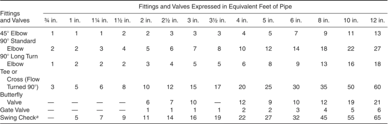
Minor losses through fittings and valves are not fric-tion losses but energy losses, caused by turbulence in the water flow which increase as the velocity of flow in-creases. Nevertheless, it has become standard practice to simplify calculation of such losses through the use of “equivalent lengths,” which are added to the actual pipe length in determining the pipe friction loss. NFPA 13 con-tains a table of equivalent pipe lengths for this purpose. (See Table 4-3.2.) As an example, if a 2-in. (50.8-mm) 90-degree long turn elbow is assigned an equivalent length of 3 ft (0.914 m), this means that the energy loss associated with turbulence through the elbow is expected to approx-imate the energy loss to friction through 0.914 m of 50.8 mm pipe. As with the friction loss tables, the equivalent pipe length chart is based on the use of steel pipe with a C-factor of 120, and the use of other piping materials re-quires multiplying factors. The equivalent pipe length for pipes having C values other then 120 should be adjusted using the following multiplication factors: 0.713 for a C value of 100; 1.16 for a C value of 130; 1.33 for a C value of 140; 1.51 for a C value of 150.
EXAMPLE 7:
If the 12-ft (3.6-m) length of 1-in. (25.4-mm) pipe in Example 6 had contained 4 elbows so as to avoid a build-ing column, the pressure loss from those elbows could be approximated by adding an equivalent length of pipe to the friction loss calculation. Table 4-3.2 gives a value of 2 ft (0.610 m) as the appropriate equivalent length for stan-dard elbows in 1 in. (25.4 mm) Schedule 40 steel pipe. For
Type of Pipe Assigned C Factor
Steel pipe—dry and preaction systems 100
Steel pipe—wet and deluge systems 120
Galvanized steel pipe—all systems 120
Cement lined cast or ductile iron 140
Copper tube 150
Plastic (listed) 150
4 elbows, the equivalent fitting length would be 8 ft (2.4 m). Added to the actual pipe length of 12 ft (3.6 m), the to-tal equivalent length would be 20 ft (6 m). This results in a new value of pfC20-ft Ý0.20 psi/ft C4.0 psi (0.28 bar). The total pressure at the second sprinkler would then be equal to 20.2 psi = 4.0 psi C24.2 psi (1.67 bar). The total flow from the second sprinkler in this case would be QC K(P)1/2C27.5 gpm (100.4 lpm).
Some types of standard valves, such as swing check valves, are included in the equivalent pipe length chart, Table 4-3.2. Equivalent lengths for pressure losses through system alarm, dry, and deluge valves are determined by the approval laboratories at the time of product listing.
Use of Velocity Pressures
The value of pressure, P, in the sprinkler orifice flow formula can be considered either the total pressure, Pt, or the normal pressure, Pn, since NFPA 13 permits the use of
velocity pressures at the discretion of the designer. Total pressure, normal pressure, and velocity pressure, Pv, have the following relationship:
PnCPt>Pv
Total pressure is the counterpart of total energy or to-tal head, and can be considered the pressure that would act against an orifice if all of the energy of the water in the pipe at that point were focused toward flow out of the ori-fice. This is the case where there is no flow past the orifice in the piping. Where flow does take place in the piping past an orifice, however, normal pressure is that portion of the total pressure which is actually acting normal to the rection of flow in the piping, and therefore acting in the di-rection of flow through the orifice. The amount by which normal pressure is less than total pressure is velocity pres-sure, which is acting in the direction of flow in the piping. Velocity pressure corresponds to velocity energy, which is the energy of motion. There is no factor in the above ex-pression for elevation head, because the flow from an ori-fice can be considered to take place in a datum plane.
When velocity pressures are used in calculations, it is recognized that some of the energy of the water is in the form of velocity head, which is not acting normal to the pipe walls (where it would help push water out the orifice), but rather in the downstream direction. Thus, for every sprinkler (except the end sprinkler on a line), slightly less flow takes place than what would be calculated from the use of the formula QCK(Pt)1/2. (See Figure 4-3.2.)
NFPA 13 permits the velocity pressure effects to be ig-nored, however, since they are usually rather minor, and since ignoring the effects of velocity pressure tends to produce a more conservative design.
If velocity pressures are considered, normal pressure rather than total pressure is used when determining flow through any sprinkler except the end sprinkler on a branch line, and through any branch line except the end branch line on a cross main. The velocity pressure, Pv, which is subtracted from the total pressure in order to de-termine the normal pressure, is dede-termined as
PvC v2
2g?0.433 psi/ft (0.098 bar/m) or
PvC0.001123Q2/d4
Fittings and Valves Expressed in Equivalent Feet of Pipe Fittings
and Valves ¾ in. 1 in. 1¼ in. 1½ in. 2 in. 2½ in. 3 in. 3½ in. 4 in. 5 in. 6 in. 8 in. 10 in. 12 in.
45ÜElbow 1 1 1 2 2 3 3 3 4 5 7 9 11 13 90ÜStandard Elbow 2 2 3 4 5 6 7 8 10 12 14 18 22 27 90ÜLong Turn Elbow 1 2 2 2 3 4 5 5 6 8 9 13 16 18 Tee or Cross (Flow Turned 90Ü) 3 5 6 8 10 12 15 17 20 25 30 35 50 60 Butterfly Valve — — — — 6 7 10 — 12 9 10 12 19 21 Gate Valve — — — — 1 1 1 1 2 2 3 4 5 6 Swing Checka — 5 7 9 11 14 16 19 22 27 32 45 55 65 For SI Units: 1 ft C0.3048 m.
aDue to the variations in design of swing check valves, the pipe equivalents indicated in the above chart are to be considered average.
Table 4-3.2 Equivalent Pipe Length Chart (for C C120)
N
N T
PR gages
Pipe
V Flow
where Q is the upstream flow through the piping to an orifice (or branch line) in gpm and d is the actual internal diameter of the upstream pipe in inches.
Because NFPA 13 mandates the use of the upstream flow, an iterative approach to determining the velocity pressure is necessary. The upstream flow cannot be known unless the flow from the sprinkler (or branch line) in question is known, and the flow from the sprinkler (or branch line) is affected by the velocity pressure resulting from the upstream flow.
EXAMPLE 8:
If the pipe on the upsteam side of the second sprin-kler in Example 6 were 3 in. Schedule 40 steel pipe with an inside diameter of 1.38 in. (35 mm), the flow from the sec-ond sprinkler would be considered to be 26.6 gpm (100.2 lpm) as determined at the end of Example 6, if velocity pressures were not included.
If velocity pressures were to be considered, an up-stream flow would first be assumed. Since the end sprin-kler had a minimum flow of 25.2 gpm (95.2 lpm) and the upstream flow would consist of the combined flow rates of the two sprinklers, an estimate of 52 gpm (196.8 lpm) might appear reasonable. Substituting this flow and the pipe diameter into the equation for velocity pressure gives
PvC
0.001123Q2
d4 C0.001123(52)(1.38)4 2 C0.8 psi (0.06 bar)
This means that the actual pressure acting on the orifice of the second sprinkler is equal to
PnCPt>Pv
C22.6 psi>0.8 psi
C21.8 psi (1.50 bar)
This would result in a flow from the second sprinkler of QCK(P)1/2
C26.1 gpm (98.7 lpm)
Combining this flow with the known flow from the end sprinkler results in a total upstream flow of 51.3 gpm (194.2 lpm). To determine if the initial guess was close enough, determine the velocity pressure that would re-sult from an upstream flow of 51.3 gpm (194.2 lpm). This calculation also results in a velocity pressure of 0.8 psi (0.06 bar), and the process is therefore complete. It can be seen that the second sprinkler apparently flows 0.5 gpm (1.9 lpm) less through the consideration of velocity pressures.
Elevation Losses
Variation of pressure within a fluid at rest is related to the density or unit (specific) weight of the fluid. The unit weight of a fluid is equal to its density multiplied by the
acceleration of gravity. The unit weight of water is 62.4 lbs/ft3(1000 kg/m3).
This means that one cubic foot of water at rest weighs 62.4 pounds (1000 kg). The cubic foot of water, or any other water column one foot high, thus results in a static pressure at its base of 62.4 pounds per square foot (304.66 kg/m2). Divided by 144 sq in. per sq ft (1.020 ?104kg/m3
bar), this is a pressure of 0.433 pounds per sq in. per ft (0.099 bar/m) of water column.
A column of water 10 ft (3.048 m) high similarly ex-erts a pressure of 10 ft ?62.4 lbs/ft2?1 ft/144 in.2C4.33
psi (3.048 m ?999.5 kg/m2@ 1.020 ?104kg/m2 bar C
0.299 bar). The static pressure at the top of both columns of water is equal to zero (gauge pressure), or atmospheric pressure.
On this basis, additional pressure must be available within a sprinkler system water supply to overcome the pressure loss associated with elevation. This pressure is equal to 0.433 psi per foot (0.099 bar/m) of elevation of the sprinklers above the level where the water supply in-formation is known.
Sometimes the additional pressure needed to over-come elevation is added at the point where the elevation change takes place within the system. If significant eleva-tion changes take place within a poreleva-tion of the system that is likely to be considered as a representative flowing orifice (such as a single branch line along a cross main that is equivalent to other lines in the remote design area), then it is considered more accurate to wait until calcula-tions have been completed, and simply add an elevation pressure increase to account for the total height of the highest sprinklers above the supply point.
EXAMPLE 9:
The pressure that must be added to a system supply to compensate for the fact that the sprinklers are located 120 ft (36.6 m) above the supply can be found by multi-plying the total elevation difference by 0.433 psi/ft (0.099 bar/m).
120 ft ?0.433 psi/ft C52 psi (3.62 bar) Loops and Grids
Hydraulic calculations become more complicated when piping is configured in loops or grids, such that water feeding any given sprinkler or branch line can be supplied through more than one route. A number of com-puter programs that handle the repetitive calculations have therefore been developed specifically for fire protec-tion systems, and are being marketed commercially.
Determining the flow split that takes place in the var-ious parts of any loop or grid is accomplished by apply-ing the basic principles of conservation of mass and conservation of energy. For a single loop, it should be rec-ognized that the energy loss across each of the two legs from one end of the system to the other must be equal. Otherwise, a circulation would take place within the loop itself. Also, mass is conserved by the fact that the sum of the two individual flows through the paths is equal to the total flow into (and out of) the loop. (See Figure 4-3.3.)
Applying the Hazen-Williams formula to each leg of the loop pfCL14.52Q 1.85 1 C1.85 1 d 4.87 1 CL24.52Q 1.85 2 C1.85 2 d 1.85 2
Substituting the term FLC for all terms except Q, pfCFLC1Q1.851 CFLC2Q1.852
This simplifies to become
ΠQ1 Q2 1.85 CFLC2 FLC1
Since Q1and Q2combine to create a total flow of Q, the
flow through one leg can be determined as
Q1C Q
[(FLC1/FLC2)0.54=1]
For the simplest of looped systems, a single loop, hand calculations are not complex. Sometimes, seemingly complex piping systems can be simplified by substituting an “equivalent pipe” for two or more pipes in series or in parallel.
For pipes in series
FLCeCFLC1=FLC2=FLC3= ß For pipes in parallel
Œ 1 FLCe 0.54 C Œ 1 FLC1 0.54 = Œ 1 FLC2 0.54 = ß
For gridded systems, which involve flow through multiple loops, computers are generally used since it be-comes necessary to solve a system of nonlinear equations. When hand calculations are performed, the Hardy Cross2
method of balancing heads is generally employed. This method involves assuming a flow distribution within the piping network, then applying successive corrective flows until differences in pressure losses through the var-ious routes are nearly equal.
The Hardy Cross solution procedure applied to sprinkler system piping is as follows:
1. Identify all loop circuits and the significant parame-ters associated with each line of the loop, such as pipe
length, diameter, and Hazen-Williams coefficient. Re-duce the number of individual pipes where possible by finding the equivalent pipe for pipes in series or parallel.
2. Evaluate each parameter in the proper units. Minor losses through fittings should be converted to equiva-lent pipe lengths. A value of all parameters except flow for each pipe section should be calculated (FLC). 3. Assume a reasonable distribution of flows that
satisi-fies continuity, proceeding loop by loop.
4. Compute the pressure (or head) loss due to friction, pf,
in each pipe using the FLC in the Hazen-Williams formula.
5. Sum the friction losses around each loop with due re-gard to sign. (Assume clockwise positive, for exam-ple.) Flows are correct when the sum of the losses, dpf, is equal to zero.
6. If the sum of the losses is not zero for each loop, di-vide each pipe’s friction loss by the presumed flow for the pipe, pf/Q.
7. Calculate a correction flow for each loop as
dQC >dpf [1.85&(pf/Q)]
8. Add the correction flow values to each pipe in the loop as required, thereby increasing or decreasing the earlier assumed flows. For cases where a single pipe is in two loops, the algebraic difference between the two values of dQ must be applied as the correction to the assumed flow.
9. With a new set of assumed flows, repeat steps 4 through 7 until the values of dQ are sufficiently small. 10. As a final check, calculate the pressure loss by any route from the initial to the final junction. A second calculation along another route should give the same value within the range of accuracy expected.
NFPA 13 requires that pressures be shown to balance within 0.5 psi (0.03 bar) at hydraulic junction points. In other words, the designer (or computer program) must continue to make successive guesses as to how much flow takes place in each piece of pipe until the pressure loss from the design area back to the source of supply is ap-proximately the same (within 0.5 psi [0.03 bar]) regardless of the path chosen.
EXAMPLE 10:
For the small two-loop grid shown in Figure 4-3.4, the total flow in and out is 100 gpm (378.5 lpm). It is necessary to determine the flow taking place through each pipe section. The system has already been simpli-fied by finding the equivalent pipe for all pipes in series and in parallel. The following values of FLC have been calculated: Pipe 1 FLCC0.001 Pipe 2 FLCC0.002 Pipe 3 FLCC0.003 Pipe 4 FLCC0.001 Pipe 5 FLCC0.004 pf Q1 Q Q Q2
Under step 3 of the Hardy Cross procedure, flows that would satisfy conservation of mass are assumed. (See Figure 4-3.5.) Steps 4 through 9 are then carried out in a tabular approach. (See Table 4-3.3.)
Making these adjustments to again balance flows, a second set of iterations can be made. (See Table 4-3.4.) For pipe segment 3, the new flow is the algebraic sum of the original flow plus the flow corrections from both loops. (See Figures 4-3.6 and 4-3.7.)
In starting the third iteration, it can be seen that the pressure losses around both loops are balanced within 0.5 psi. (See Table 4-3.5.) Therefore, the flow split assumed af-ter two iaf-terations can be accepted. As a final check, step 10 of the above procedure calls for a calculation of the total pressure loss through two different routes, requiring that they balance within 0.5 psi (0.03 bar):
Route through pipes 1 and 5: FLC1, (Q1)1.85=FLC2(Q2)1.85
C0.001(54.0)1.85=0.004(35.9)1.85 C1.6=3.0C4.6 psi (0.32 bar) Route through Pipes 2 and 4:
0.002(46.0)1.85=0.001(64.1)1.85C2.4=2.2 C4.6 psi (0.32 bar) This is acceptable. Note that it required only two itera-tions to achieve a successful solution despite the fact that the initial flow assumption called for reverse flow in pipe 3. The initial assumption was for a clockwise flow of 5 gpm (18.9 lpm) in pipe 3, but the final solution shows a counterclockwise flow of 18.1 gpm (68.5 lpm). Loop 1 2 Pipe 1 2 3 3 4 5 Q –40 60 5 –5 55 –45 FLC 0.001 0.002 0.003 0.003 0.001 0.004 pf –0.92 3.90 0.06 –0.06 1.66 –4.58 dpf C 3.04 C–2.98 (pf/Q) 0.023 0.065 0.012 0.100 0.012 0.030 0.102 0.144 dQC–dpf/1.85[ | (pf/Q)] dQC–16.4 dQC11.2 Q=dQ –56.4 =43.6 –11.4 =6.2 =66.2 =33.8
Table 4-3.3 First Iteration
Loop 1 2 Pipe 1 2 3 3 4 5 Q –56.4 43.6 –22.6 22.6 66.2 –33.8 FLC 0.001 0.002 0.003 0.003 0.001 0.004 pf –1.74 2.16 –0.96 0.96 2.34 –2.69 dpf C–0.54 C 0.61 (pf/Q) 0.031 0.050 0.042 0.123 0.042 0.035 0.080 0.157 dQC–dpf/1.85[|(pf/Q)] dQC2.4 dQC–2.1 Q=dQ –54.0 =46.0 –20.2 =20.5 =64.1 =35.9
Table 4-3.4 Second Iteration
5
45 Loop 1
Original flow assumptions Loop 2 100 gpm 40 55 60 100 gpm + +
Figure 4-3.5. Original flow assumptions.
2 4 5 1 3 Loop 1 Simplified system Loop 2 100 gpm 100 gpm
Water Supply Calculations
Determination of Available Supply CurveTesting a public or private water supply permits an evaluation of the strength of the supply in terms of both quantity of flow and available pressures. The strength of a water supply is the key to whether it will adequately serve a sprinkler system.
Each test of a water supply must provide at least two pieces of information—a static pressure and a residual pressure at a known flow. The static pressure is the “no flow” condition, although it must be recognized that rarely is any public water supply in a true no flow condi-tion. But this condition does represent a situation where the fire protection system is not creating an additional flow demand beyond that which is ordinarily placed on the system. The residual pressure reading is taken with an additional flow being taken from the system, prefer-ably a flow that approximates the likely maximum sys-tem demand.
Between the two (or more) points, a representation of the water supply (termed a water supply curve) can be made. For the most part, this water supply curve is a fingerprint of the system supply and piping arrange-ments, since the static pressure tends to represent the ef-fect of elevated tanks and operating pumps in the system, and the drop to the residual pressure represents the fric-tion and minor losses through the piping network that re-sult from the increased flow during the test.
The static pressure is read directly from a gauge at-tached to a hydrant. The residual pressure is read from the same gauge while a flow is taken from another
hy-drant, preferably downstream. A pitot tube is usually used in combination with observed characteristics of the nozzle though which flow is taken in order to determine the amount of flow. Chapter 7 of NFPA 13 provides more thorough information on this type of testing.
Figure A-8-3.2(d) of NFPA 13 (1999 edition) is an ex-ample of a plot of water supply information. The static pressure is plotted along the y-axis, reflecting a given pressure under zero flow conditions. The residual pres-sure at the known flow is also plotted, and a straight line is drawn between these two points. Note that the x-axis is not linear, but rather shows flow as a function of the 1.85 power. This corresponds to the exponent for flow in the Hazen-Williams equation. Using this semi-exponential graph paper demonstrates that the residual pressure ef-fect is the result of friction loss through the system, and permits the water supply curve to be plotted as a straight line. Since the drop in residual pressure is proportional to flow to the 1.85 power, the available pressure at any flow can be read directly from the water supply curve.
For adequate design, the system demand point, in-cluding hose stream allowance, should lie below the wa-ter supply curve.
EXAMPLE 11:
If a water supply is determined by test to have a sta-tic pressure of 100 psi (6.9 bar) and a residual pressure of 80 psi (5.5 bar) at a flow of 1000 gpm (3785 lpm), the pres-sure available at a flow of 450 gpm (1703 lpm) can be ap-proximated by plotting the two known data points on the hydraulic graph paper as shown in Figure 4-3.8. At a flow of 450 gpm (1703 lpm), a pressure of 90 psi (6.2 bar) is indicated. Loop 1 2 Pipe 1 2 3 3 4 5 Q –54.0 46.0 –18.1 18.1 64.1 –35.9 FLC 0.001 0.002 0.003 0.003 0.001 0.004 pf –1.60 2.38 –0.64 0.64 2.20 –3.01 dpf C 0.14 C–0.17 (pf/Q) dQC–dpf/1.85[ | (pf/Q)] Q=dQ
Table 4-3.5 Third Iteration 22.6 33.8 100 gpm 56.4 66.2 43.6 100 gpm
Figure 4-3.6. Corrected flows after first iteration.
18.1 35.9 100 gpm 54.0 64.1 46.0 100 gpm
Pump Selection and Testing
Specific requirements for pumps used in sprinkler sys-tems are contained in NFPA 20, which is cross-referenced by NFPA 13.
Fire pumps provide a means of making up for pres-sure deficiencies where an adequate volume of water is available at a suitable net positive suction pressure. Plumbing codes sometimes set a minimum allowable net positive suction pressure of 10 to 20 psi (0.69 to 1.38 bar). If insufficient water is available at such pressures, then it becomes necessary to use a stored water supply.
Listed fire pumps are available with either diesel or electric drivers, and with capacities ranging from 25 to 5000 gpm (95 to 18,927 lpm), although fire pumps are most commonly found with capacities ranging from 250 to 2500 gpm (946 to 9463 lpm) in increments of 250 up to 1500 gpm (946 up to 5678 lpm) and 500 gpm (1893 lpm) beyond that point. Each pump is specified with a rated flow and rated pressure. Rated pressures vary exten-sively, since manufacturers can control this feature with small changes to impeller design.
Pump affinity laws govern the relationship between impeller diameter, D, pump speed, N, flow, Q, pressure head, H, and brake horsepower, bhp. The first set of affin-ity laws assumes a constant impeller diameter.
Q1 Q2C N1 N2 H1 H2C N1 N2 bhp1 bhp2C N1 N2
These affinity laws are commonly used when correct-ing the output of a pump to its rated speed.
The second set of the affinity laws assumes constant speed with change in impeller diameter, D.
Q1 Q2C D1 D2 H1 H2C D1 D2 bhp1 bhp2C D1 D2
Pumps are selected to fit the system demands on the basis of three key points relative to their rated flow and rated pressure. (See Figure 4-3.9.) NFPA 20 specifies that each horizontal fire pump must meet these characteris-tics, and the approval laboratories ensure these points are met:
1. A minimum of 100 percent of rated pressure at 100 per-cent of rated flow.
2. A minimum of 65 percent of rated pressure at 150 per-cent of rated flow.
3. A maximum of 140 percent of rated pressure at 0 per-cent of rated flow (churn).
Even before a specific fire pump has been tested, therefore, the pump specifier knows that a given pump can be expected to provide certain performance levels. It is usually possible to have more than one option when choosing pumps, since the designer is not limited to using a specific point on the pump performance curve.
There are limits to flexibility in pump selection, however. For example, it is not permitted to install a pump in a situation where it would be expected to oper-ate with a flow exceeding 150 percent of roper-ated capacity, since the performance is not a known factor, and indeed available pressure is usually quick to drop off beyond this point.
NFPA 20 gives the following guidance on what part of the pump curve to use:1
A centrifugal fire pump should be selected in the range of operation from 90 percent to 150 percent of its rated capacity. The performance of the pump when applied at capacities over 140 percent of rated capacity may be adversely af-fected by the suction conditions. Application of the pump at capacities less than 90 percent of the rated capacity is not recommended.
The selection and application of the fire pump should not be confused with pump oper-ating conditions. With proper suction conditions, the pump can operate at any point on its charac-teristic curve from shutoff to 150 percent of its rated capacity.
For design capacities below the rated capacity, the rated pressure should be used. For design capacities be-tween 100 and 150 percent of rated capacity, the pressure 100 90 60 PSI Flow (gpm) 450 1000
Figure 4-3.8. Pressure available from 450 gpm flow
water supply. 140 120 100 80 60 40 20 50 100
Percent of rated capacity
P ercent of total r ated head 150 200 0 Rated capacity Total rated head
used should be found by the relationship made apparent by similar triangles. 0.35P 0.5Q C P>0.65P 1.5Q>Q
where P and Q are the rated pressure and capacity, and P is the minimum available pressure at capacity, Q, where QAQA1.5Q.
EXAMPLE 12:
A pump is to be selected to meet a demand of 600 gpm (2271 lpm) at 85 psi (5.86 bar). To determine whether a pump rated for 500 gpm (1893 lpm) at 100 psi (6.90 bar) would be able to meet this point without having an actual pump performance curve to work from, the above for-mula can be applied, with PC100,QC500, and QC600.
Inserting these values gives (0.35)(100) (0.5)(500) C [P>(0.65)(100)] [(1.5)(500)>600] 35 250C (P>65) (750>600) PC65=21C86 psi (5.93 bar)
Since the value of Pso calculated is greater than the 85 psi (5.86 bar) required, the pump will be able to meet the demand point.
Tank Sizing
Tank selection and sizing are relatively easy com-pared to pump selection. The most basic question is whether to use an elevated storage (gravity) tank, a pres-sure tank, or a suction tank in combination with a pump. Following that is a choice of materials. NFPA 22 is the governing standard for water tanks for fire protection, and includes a description of the types of tanks as well as detailed design and connection requirements.
From a calculation standpoint, tanks must be sized to provide the minimum durations specified by NFPA 13 or other applicable standards for the system design. Re-quired pressures must still be available when the tanks are at the worst possible water level condition (i.e., nearly empty).
If the tank is intended to provide the needed supply without the use of a pump, the energy for the system must be available from the height of a gravity tank or the air pressure of a pressure tank.
An important factor in gravity tank calculations is the requirement that the pressure available from elevation [calculated using 0.433 psi per foot (0.099 bar/m)] must be determined using the lowest expected level of water in the tank. This is normally the point at which the tank would be considered empty.
In sizing pressure tanks, the percentage of air in the tanks must be controlled so as to ensure that the last wa-ter leaving the tank will be at an adequate pressure. While a common rule of thumb has been that the tank should be one-third air at a minimum pressure of 75 psi (5.17 bar), this rule does not hold true for systems with high
pres-sure demands or where the tank is located a considerable distance below the level of the highest sprinkler.
For pipe schedule systems, two formulas have tradi-tionally been used, based on whether the tank is located above the level of the highest sprinkler or some distance below.
For the tank above the highest sprinkler PC30
A >15
For the tank below the highest sprinkler
PC ‹ 30 A >15 = ‹ 0.434H A where
ACproportion of air in the tank
PCair pressure carried in the tank in psi
HCheight of the highest sprinkler above the tank bottom in feet
It can be seen that these formulas are based simply on the need to provide a minimum pressure of 15 psi (1.03 bar) to the system at the level of the highest sprin-kler, and an assumption of 15 psi (1.03 bar) atmospheric pressure.
Using the same approximation for atmospheric pres-sure, a more generalized formula has come into use for hydraulically designed systems:
PiC
Pf=15 A >15 where
PiCtank air pressure to be used
PfCsystem pressure required per hydraulic calculations
ACproportion of air in the tank EXAMPLE 13:
A pressure tank is to be used to provide a 30-min-water supply to a system with a hydraulically calculated demand of 140 gpm (530 lpm) at a pressure of 118 psi (8.14 bar). Since there are sprinklers located adjacent to the tank, it is important that air pressure in the tank not ex-ceed 175 psi (12.0 bar). To determine the minimum size tank that can be used, it is important not only to consider the total amount of water needed, but also the amount of air necessary to keep the pressures within the stated limits.
The above equation for hydraulically designed sys-tems can be used to solve for A.
If PiC ” ˜ (Pf=15) A >15 then AC(Pf=15) (Pi=15) AC(118=15) (175=15)C 133 190C0.70
This means that the tank will need to be 70 percent air if the air pressure in the tank is to be kept to 175 psi (12.0 bar).
The minimum water supply required is 30 min ?140 gpm C4200 gallons (15,898 l).
Thus, the minimum tank volume will be such that 4200 gallons (15,898 l) can be held in the remaining 30 per-cent of volume.
0.3VC4200 gal VC42000.3 C14,000 gal tank (53,000 l)
Hanging and Bracing Methods
Hangers and Hanger SupportsNFPA 13 contains a great deal of specific guidance relative to hanger spacing and sizing based on pipe sizes. It should also be recognized that the standard al-lows a performance-based approach. Different criteria exist for the hanger itself and the support from the build-ing structure.
Any hanger and installation method is acceptable if certified by a registered professional engineer for the following:
1. Hangers are capable of supporting five times the weight of the water-filled pipe plus 250 pounds (114 kg) at each point of piping support.
2. Points of support are sufficient to support the sprinkler system.
3. Ferrous materials are used for hanger components. The building structure itself must be capable of sup-porting the weight of the water-filled pipe plus 250 pounds (114 kg) applied at the point of hanging.
The 250 pound (114 kg) weight is intended to repre-sent the extra loading that would occur if a relatively heavy individual were to hang on the piping.
Trapeze Hangers
Trapeze hangers are used where structural members are not located, so as to provide direct support of sprin-kler lines or mains. This can occur when sprinsprin-kler lines or mains run parallel to structural members such as joists or trusses.
A special section of NFPA 13 addresses the sizing of trapeze hangers. Because they are considered part of the support structure, the criteria within NFPA 13 are based on the ability of the hangers to support the weight of 15 ft (5 m) of water-filled pipe plus 250 pounds (114 kg) applied at the point of hanging. An allowable stress of 15,000 psi (111 bar) is used for steel members. Two tables are pro-vided in the standard, one of which presents required sec-tion moduli based on the span of the trapeze and the size and type of pipe to be supported, and the other of which presents the available section moduli of standard pipes and angles typically used as trapeze hangers.
In using the tables, the standard allows the effective span of the trapeze hanger to be reduced if the load is not at the midpoint of the span. The equivalent length of trapeze is determined from the formula
LC(a4=abb)
where Lis the equivalent length, a is the distance from one support to the load, and b is the distance from the other support to the load.
EXAMPLE 14:
A trapeze hanger is required for a main running par-allel to two beams spaced 10 ft (3.048 m) apart. If the main is located 1 ft 6 in. (0.457 m) from one of the beams, the equivalent span of trapeze hanger required can be determined by using the formula
LC4(1.5 ft)(8.5 ft)(1.5 ft=8.5 ft)C5.1 ft (1.554 m) Earthquake Braces
Protection for sprinkler systems in earthquake areas is provided in several ways. Flexibility and clearances are added to the system where necessary to avoid the devel-opment of stresses that could rupture the piping. Too much flexibility could also be dangerous, however, since the momentum of the unrestrained piping during shak-ing could result in breakage of the pipshak-ing under its own weight or upon collision with other building components. Therefore, bracing is required for large piping (including all mains) and for the ends of branch lines.
Calculating loads for earthquake braces is based on the assumption that the normal hangers provided to the system are capable of handling vertical forces, and that horizontal forces can be conservatively approximated by a constant acceleration equal to one-half that of gravity.
ahC0.5g
NFPA 13 contains a table of factors that can be ap-plied if building codes require the use of other horizontal acceleration values.
Since the braces can be called upon to act in both ten-sion and compresten-sion, it is necessary not only to size the brace member to handle the expected force applied by the weight of the pipe in its zone of influence, but also to avoid a member that could fail as a long column under buckling.
The ability of the brace to resist buckling is deter-mined through an application of Euler’s formula with a maximum slenderness ratio of 300. This corresponds to the maximum slenderness ratio generally used under steel construction codes for secondary framing members. This is expressed as
Ú
r D300
where Ú Clength of the brace and rCleast radius of gy-ration for the brace.
The least radius of gyration for some common shapes is as follows: pipe rC(r 2 0=ri2)1/2 2 rod rCr 2 flat rC0.29h
Special care must be taken in the design of earth-quake braces so that the load applied to any brace does not exceed the capability of the fasteners of that brace to the piping system or the building structure, and that the braces are attached only to structural members capable capable of supporting the expected loads.
Performance Calculations
Sprinkler Response as a DetectorAutomatic sprinklers serve a dual function as both heat detectors and water distribution nozzles. As such, the response of sprinklers can be estimated using the same methods as for response of heat detectors. (See Sec-tion 4, Chapter 1.) Care should be taken, however, since the use of such calculations for estimating sprinkler actu-ation times has not been fully established. Factors, such as sprinkler orientation, air flow deflection, radiation effects, heat of fusion of solder links, and convection within glass bulbs, are all considered to introduce minor errors into the calculation process. Heat conduction to the sprinkler frame and distance of the sensing mechanism below the ceiling have been demonstrated to be significant factors affecting response, but are ignored in some computer models.
Nevertheless, modeling of sprinkler response can be useful, particularly when used on a comparative basis. Beginning with the 1991 edition, an exception within Sec-tion 4-1.1 of NFPA 13 permitted variaSec-tions from the rules on clearance between sprinklers and ceilings “ . . . pro-vided the use of tests or calculations demonstrate compa-rable sensitivity and performance.”
EXAMPLE 15:
Nonmetallic piping extending 15 in. (0.38 m) below the concrete ceiling of a 10-ft- (3.048 m-) high basement 100 ft by 100 ft (30.48 ?30.48 m) in size makes it difficult to place standard upright sprinklers within the 12 in. (0.30 m) required by NFPA 13 for unobstructed construction. Using the LAVENT9computer model, and assuming RTI
values of 400 ft1/2Ýs1/2(221 m1/2Ýs1/2) for standard
sprin-klers and 100 ft1/2Ýs1/2(55 m1/2Ýs1/2) for quick-response
sprinklers, it can be demonstrated that the comparable level of sensitivity can be maintained at a distance of 18 in. (0.457 m) below the ceiling. Temperature rating is as-sumed to be 165ÜF, and maximum lateral distance to a sprinkler is 8.2 ft (2.50 m) (10 ft ?13 ft [3.048 m ?3.962 m] spacing). Assuming the default fire (empty wood pallets stored 5 ft [1.52 m] high), for example, the time of actua-tion for the standard sprinkler is calculated to be 200 s, as compared to 172 s for the quick-response sprinkler. Since the noncombustible construction minimizes concern rela-tive to the fire control performance for the structure, the sprinklers can be located below the piping obstructions.
Dry System Water Delivery Time
Total water delivery time consists of two parts. The first part is the trip time taken for the system air pressure to bleed down to the point where the system dry valve
opens to admit water to the piping. The second part is the transit time for the water to flow through the piping from the dry valve to the open sprinkler. In other words
water delivery time Ctrip time =transit time where water delivery time commences with the opening of the first sprinkler.
NFPA 13 does not contain a maximum water delivery time requirement if system volume is held to no more than 750 gal (2839 l). Larger systems are permitted only if water delivery time is within 60 s. As such, the rule of thumb for dry system operation is that no more than a 60 s water delivery time should be tolerated, and that sys-tems should be divided into smaller syssys-tems if necessary to achieve this 1-min response. Dry system response is simulated in field testing by the opening of an inspector’s test connection. The test connection is required to be at the most remote point of the system from the dry valve, and is required to have an orifice opening of a size simu-lating a single sprinkler.
The water delivery time of the system is recorded as part of the dry pipe valve trip test that is conducted using the inspector’s test connection. However, it is not a realistic indication of actual water delivery time for two reasons:
1. The first sprinkler to open on the system is likely to be closer to the system dry valve, reducing water transit time.
2. If additional sprinklers open, the trip time will be re-duced since additional orifices are able to expel air. Water transit time may also be reduced since it is easier to expel the air ahead of the incoming water.
Factory Mutual Research Corporation (FMRC) re-searchers have shown3that it is possible to calculate
sys-tem trip time using the relation
tC0.0352 VT AnT1/2 0 ln Πpa0 pa where tCtime in seconds
VTCdry volume of sprinkler system in cubic feet T0Cair temperature in Rankine degrees
AnCflow area of open sprinklers in square feet
pa0Cinitial air pressure (absolute)
paCtrip pressure (absolute)
Calculating water transit time is more difficult, but may be accomplished using a mathematical model de-veloped by FMRC researchers. The model requires the system to be divided into sections, and may therefore pro-duce slightly different results, depending on user input.
Droplet Size and Motion
For geometrically similar sprinklers, the median drop-let diameter in the sprinkler spray has been found to be in-versely proportional to the 1/
directly proportional to the 2/
3power of sprinkler orifice
diameter such that
dmä D2/3 P1/3 ä D2 Q2/3 where
dmCmean droplet diameter
DCorifice diameter PCpressure
QCrate of water flow
Total droplet surface area has been found to be pro-portional to the total water discharge rate divided by the median droplet diameter
ASä
Q dm
where ASis the total droplet surface area.
Combining these relationships, it can be seen that ASä(Q3pD>2)1/3
When a droplet with an initial velocity vector of U is dri-ven into a rising fire plume, the one-dimensional repre-sentation of its motion has been represented as4
m1dU
dt Cm1g>
CD:g(U=V)2
2S where
UCvelocity of the water droplet VCvelocity of the fire plume mCmass of the droplet :gCdensity of the gas
gCacceleration of gravity CDCcoefficient of drag
SfCfrontal surface area of the droplet
The first term on the right side of the equation sents the force of gravity, while the second term repre-sents the force of drag caused by gas resistance. The drag coefficient for particle motion has been found empirically to be a function of the Reynolds number (Re) as5
CDC18.5 Re>0.6 for ReA600
CDC0.44 for ReB600
Spray Density and Cooling
The heat absorption rate of a sprinkler spray is ex-pected to depend on the total surface area of the water droplets, AS, and the temperature of the ceiling gas layer in excess of the droplet temperature, T. With water tem-perature close to ambient temtem-perature, T can be consid-ered excess gas temperature above ambient.
Chow6 has developed a model for estimating the
evaporation heat loss due to a sprinkler water spray in a smoke layer. Sample calculations indicate that evapora-tion heat loss is only significant for droplet diameters less
than 0.5 mm. For the droplet velocities and smoke layer depths analyzed, it was found that the heat loss to evapo-ration would be small (10 to 25 percent), compared to the heat loss from convective cooling of the droplets.
Factory Mutual Research Corporation researchers7
have developed empirical correlations for the heat ab-sorption rate of sprinkler spray in room fires, as well as convective heat loss through the room opening, such that
Qg CQgcool=Qg =c Qgl where
Qg Ctotal heat release rate of the fire
QgcoolCheat absorption rate of the sprinkler spray Qg Cc convective heat loss rate through the room opening
Qg Cl sum of the heat loss rate to the walls and ceiling,
Qgs, the heat loss rate to the floor, Qgf, and the
ra-diative heat loss rate through the opening, Qgr Test data indicated that
Qgcool/Qg C0.000039#3>0.003#2=0.082#
for 0A#D33l/(min?kW1/2?m5/4)
where #is a correlation factor incorporating heat losses to the room boundaries and through openings as well as to account for water droplet surface area.
#C(AH1/2Q l g )>1/2(W3PD>2)1/3 for PC p (17.2 kPa) and DC d 0.0111 m where
ACarea of the room opening in meters HCheight of the room opening in meters
PCwater pressure at the sprinkler in bar dCsprinkler nozzle diameter in meters WCwater discharge in liters per minute
The above correlations apply to room geometry with length-to-width ratio of 1.2 to 2 and opening size of 1.70 to 2.97 m2.
Suppression by Sprinkler Sprays
Researchers at the National Institute of Standards and Technology (NIST) have developed a “zeroth order” model of the effectiveness of sprinklers in reducing the heat release rate of furnishing fires.8Based onmeasure-ments of wood crib fire suppression with pendant spray sprinklers, the model is claimed to be conservative. The model assumes that all fuels have the same degree of re-sistance to suppression as a wood crib, despite the fact that tests have shown furnishings with large burning sur-face areas can be extinguished easily compared to the deep-seated fires encountered with wood cribs.
The recommended equation, which relates to fire sup-pression for a 610-mm-high crib, has also been checked for validity with 305-mm crib results. The equation is
Qg(t>tact)CQg(tact)exp
” ˜
>(t>tact) 3.0(wg)>1.85
where
Qg Cthe heat release rate (kW)
tCany time following tact of the sprinklers (s)
wgCthe spray density (mm/s)
The NIST researchers claim the equation is appropri-ate for use where the fuel is not shielded from the wappropri-ater spray, and the application density is at least 0.07 mm/s [4.2 mm/min. (0.1 gpm/ft2)]. The method does not
ac-count for variations in spray densities or suppression ca-pabilities of individual sprinklers.
The model must be used with caution, since it was developed on the basis of fully involved cribs. It does not consider the possibility that the fire could continue to grow in intensity following initial sprinkler discharge, and, for that reason, should be restricted to use in light hazard applications.
Sprinklers are assumed to operate within a room of a light hazard occupancy when the total heat release rate of the fire is 500 kW. The significance of an initial applica-tion rate of 0.3 gpm/ft2(0.205 mm/s) as compared to the
minimum design density of 0.1 gpm/ft2(0.07 mm/s) can
be evaluated by the expected fire size after 30 s. With the minimum density of 0.07 mm/s (0.1 gpm/ft2), the fire
size is conservatively estimated as 465 kW after 30 s. With the higher density of 0.205 mm/s (0.3 gpm/ft2), the fire
size is expected to be reduced to 293 kW after 30 s. Cor-responding values after 60 s are 432 kW and 172 kW, respectively.
Nomenclature
C coefficient of friction FLC friction loss coefficient Q flow (gpm)
wg spray density (mm/s)
References Cited
1. NFPA Codes and Standards, National Fire Protection Associa-tion, Quincy, MA.
2. H. Cross, Analysis of Flow in Networks of Conduits or Conductors, Univ. of Illinois Engineering Experiment Station, Urbana, IL (1936).
3. G. Heskested and H. Kung, FMRC Serial No. 15918, Factory Mutual Research Corp., Norwood, MA (1973).
4. C. Yao and A.S. Kalelkar, Fire Tech., 6, 4 (1970).
5. C.L. Beyler, “The Interaction of Fire and Sprinklers,”NBS GCR 77-105, National Bureau of Standards, Washington, DC (1977).
6. W.K. Chow, “On the Evaporation Effect of a Sprinkler Water Spray,” Fire Tech., pp. 364–373 (1989).
7. H.Z. You, H.C. Kung, and Z. Han, “Spray Cooling in Room Fires,” NBS GCR 86-515, National Bureau of Standards, Washington, DC (1986).
8. D.D. Evans, “Sprinkler Fire Suppression Algorithm for HAZARD,” NISTIR 5254, National Institute of Standards and Technology, Gaithersburg, MD (1993).
9. W.D. Davis and L.Y. Cooper, “Estimating the Environment and Response of Sprinkler Links in Compartment Fires with Draft Curtains and Fusible-Link Actuated Ceiling Vents, Part 2: User Guide for the Computer Code LAVENT,” NISTIR/ 89-4122, National Institute of Standards and Technology, Gaithersburg, MD (1989).