American University in Cairo American University in Cairo
AUC Knowledge Fountain
AUC Knowledge Fountain
Theses and Dissertations
2-1-2016
Determinants of stock returns: Evidence from Egypt
Determinants of stock returns: Evidence from Egypt
Reem Abd El Maksoud Ahmed El AbdFollow this and additional works at: https://fount.aucegypt.edu/etds Recommended Citation
Recommended Citation
APA Citation
El Abd, R. (2016).Determinants of stock returns: Evidence from Egypt [Master’s thesis, the American University in Cairo]. AUC Knowledge Fountain.
https://fount.aucegypt.edu/etds/326
MLA Citation
El Abd, Reem Abd El Maksoud Ahmed. Determinants of stock returns: Evidence from Egypt. 2016. American University in Cairo, Master's thesis. AUC Knowledge Fountain.
https://fount.aucegypt.edu/etds/326
This Thesis is brought to you for free and open access by AUC Knowledge Fountain. It has been accepted for inclusion in Theses and Dissertations by an authorized administrator of AUC Knowledge Fountain. For more information, please contact mark.muehlhaeusler@aucegypt.edu.
The American University in Cairo School of Business
Determinants of Stock Returns: Evidence from Egypt A Thesis Submitted to
The Department of Management
in partial fulfillment of the requirements for the Degree of
MASTER OF SCIENCE IN FINANCE
by
REEM ABD EL MAKSOUD EL ABD Under the supervision of
Dr. ALIAA BASSIOUNY December/2016
ii
DEDICATION
To my parents Sawsan and Abd El Maksoud.
iii
ACKNOWLEDGEMENTS
I would like to thank Dr Aliaa Bassiouny for her ongoing help and support. Also I’m grateful to my reviewers Dr Neveen Ahmed and Dr Khouzeima Moutanabbir for their insightful comments.
iv
The American University in Cairo School of Business
Management Department
Determinants of Stock Returns: Evidence from Egypt By
Reem Abd El Maksoud El Abd
Under the supervision of Dr. Aliaa Bassiouny ABSTRACT
This paper aims at identifying the determinants of stock returns in the Egyptian stock market. It does so by means of applying four different asset pricing models to the Egyptian stock returns: the CAPM, Fama-French three-factor model, Carhart four-factor model, and Fama-French five-four-factor model. The main findings of this thesis are that there is a significant size effect in the Egyptian stock returns, but there is no evidence of the presence of value or momentum effects. The results for operating profitability and investment are mixed therefore they need to be investigated further. Also, this paper provides evidence of the superiority of Fama-French five-factor model relative to the other asset pricing models tested.
v
TABLE OF CONTENTS
CHAPTER I ... 1
INTRODUCTION ... 1
1.1 Overview of asset pricing models ... 1
CHAPTER II ... 4
LITERATURE REVIEW ... 4
2.1 From Markowitz Portfolio Theory to Fama-French Five-Factor Model ... 4
2.2 International Tests of Asset Pricing Models ... 10
2.3 Studies conducted on the Egyptian Stock Market ... 14
2.4 The Contribution of this thesis ... 16
CHAPTER III ... 18
METHODOLOGY ... 18
3.1 Asset Pricing Models ... 18
3.2 Portfolio Construction ... 19
3.3 The GRS test ... 23
CHAPTER IV... 24
DATA AND SUMMARY STATISTICS ... 24
4.1 Data ... 24
4.2 Variables Definitions ... 25
4.3 The Number of Stocks used in each one of the different RHS and LHS portfolios... 26
4.4 Summary Statistics ... 30
CHAPTER V ... 36
RESULTS ... 36
5.1 The Results of the CAPM ... 36
5.2 The Results of Fama-French three-factor model ... 41
5.3 The Results of Carhart four-factor model ... 42
5.4 The Results of Fama-French five-factor model ... 46
5.5The Results of the GRS test ... 52
CHAPTER VI... 53
CONCLUSIONS ... 53
REFERENCES ... 54
vi
TABLES
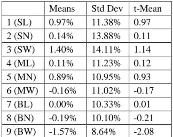
Table 1: Number of stocks in each one of the RHS Size-BM portfolios each year .... 26 Table 2: Number of stocks in each one of the LHS Size-BM portfolios each year ... 26 Table 3: Number of stocks in each one of the RHS Size-Momentum portfolios each year ... 27 Table 4: Number of stocks in each one of the LHS Size-Momentum portfolios each year ... 27 Table 5: Number of stocks in each one of the RHS Size-OP portfolios each year... 28 Table 6: Number of stocks in each one of the LHS Size-OP portfolios each year ... 28 Table 7: Number of stocks in each one of the RHS Size-Investment portfolios each year ... 29 Table 8: Number of stocks in each one of the LHS Size-Investment portfolios each year ... 29 Table9: Summary statistics of explanatory variables used in CAPM, Fama-French 3-factor model, and Carhart model ... 30 Table 10: Summary statistics of explanatory variables used in Fama-French five-factor model ... 31 Table 11: Correlation matrix between the explanatory variables used in CAPM, Fama-French three-factor model, and Carhart model ... 31 Table 12: Correlation matrix between the explanatory variables used in Fama-French five-factor model ... 31 Table 13: Summary statistics for the dependent variable (excess returns over the risk-free rate) for Size-BM portfolios ... 32 Table 14: Summary statistics for the dependent variable (excess returns over the risk-free rate) for Size-Momentum portfolios ... 33 Table 15: Summary statistics for the dependent variable (excess returns over the risk-free rate) for Size-OP portfolios ... 34 Table 16: Summary statistics for the dependent variable (excess returns over the risk-free rate) for Size-Investment portfolios ... 35
vii
Table 17: The results of the CAPM using Size-BM portfolios to construct the
dependent variables ... 37 Table 18: The results of the CAPM using Size-Momentum portfolios to construct the dependent variables ... 38 Table 19: The results of the CAPM using Size-OP portfolios to construct the
dependent variables ... 39 Table 20: The results of the CAPM using Size-Investment portfolios to construct the dependent variables ... 40 Table 21: The results of Fama-French three-factor model ... 43 Table 22: Results of Carhart model when Size-BM portfolios are used to construct the dependent variables ... 44 Table 23: Results of Carhart model when Size-Momentum portfolios are used to construct the dependent variable ... 45 Table 24: Results of Fama-French five-factor model when Size-BM portfolios are used to construct the dependent variables ... 49 Table 25: Results of Fama-French five-factor model when Size-OP portfolios are used to construct the dependent variables ... 500 Table 26: Results of Fama-French five-factor model when Size-Investment portfolios are used to construct the dependent variables ... 511 Table 27: The results of the GRS test and the SR(α) ... 52
CHAPTER 1 INTRODUCTION
1.1Overview of asset pricing models
Asset pricing models have always been a central focus of Finance literature and research. The reason for their importance is that they attempt to explain the variation in the cross-section of stock returns by means of regressing different stock portfolios on other risk-factor mimicking portfolios.
Understanding the determinants of stock returns has several practical uses. Firstly, by understanding the determinants of stock returns and the associated risks, investors (or their advisors) can perform portfolio construction and asset selection activities in a manner that maximizes their utility. Secondly, asset pricing models can be used to set benchmarks for portfolio performance; either by means of comparing the performance of different investors’ portfolios over a given time period or analyzing different portfolios’ performance over time. Thirdly, asset pricing models can guide and justify the choice of the appropriate discount rates used in capital budgeting decisions. One of the very popular methods of asset valuation is the Discounted Cash Flow (DCF) method which estimates asset values by forecasting future cash flows then calculating their present value by discounting these cash flows to the present using a discount rate that reflects their risk. Also decision makers often use hurdle rates to choose among new projects or to perform replace-or-renew analysis to existing projects or assets. The most widely used asset pricing model is the Nobel Prize winning Capital Asset Pricing Model (CAPM) that was first derived by Sharpe (1964) and Lintner (1965b) based on the model of portfolio choice that was developed in 1959 by Markowitz. In this model, investors earn a return in time t due to investing in a pre-selected portfolio in time t-1. Markowitz model assumes that investors are risk-averse and that the portfolios that they construct are mean-variance efficient. According to the CAPM, an investor investing in asset i expects to earn 𝑅𝑖 which is composed of a risk-free rate of return plus a risk premium that is a compensation for taking additional risk.
2
The CAPM represents the cornerstone of asset pricing models. Even though five decades have passed since it has been issued, it is still widely used by industry practitioners and academics. The reason for its popularity is that it offers powerful insights as to how to measure risk, and how risk and expected returns are related. Nevertheless, Fama and French (2004) argue that the CAPM suffers from empirical problems that may be due to having overly simplifying assumptions or to difficulties in performing sound tests on the model. In 1993, Fama and French construct a three-factor model that adds two additional three-factors to the market three-factor of the CAPM: a size factor and a value factor. Although Fama-French three-factor model captures the variation in stock returns due to size and book to market factors better than the CAPM, Fama and French (1993) describe the three-factor model as being far from complete. Subsequently, in 1997, Carhart being motivated by Fama and French (1996) findings, that Fama-French three-factor model isn’t able to capture the continuation of short-term returns pattern that is documented by Jagadeesh and Titman (1993), adds a momentum factor to the three-factor model to enable it to capture this momentum pattern in stock returns. For years after that, Fama-French three factor model and Carhart four factor model have been extensively used in the US, in other developed and developing countries, and recently in developed and emerging market regions as well. Nevertheless, Avramov et al. (2006) find that Carhart four-factor model isn’t able to capture all the momentum in average stock returns in the US market.
Afterwards, influenced by the dividend discount model, and the fact that many researchers have found profitability and investment patterns in stock returns in the US as well as in international markets, Fama and French (2015a) add two additional factors to the three-factor model: a profitability factor and an investment factor, to enable it to better capture the variation in stock returns. The most striking finding of Fama and French (2015a) is that adding profitability and investment factors to the three-factor model, makes the HML factor redundant. Even though the significance of the HML factor has been well established via numerous studies conducted in the US as well as worldwide.
This thesis attempts to use different asset pricing models to capture the variation in stock returns in the Egyptian market. This thesis applies the CAPM, Fama and French
3
three-factor model, Carhart four-factor model and Fama and French five-factor model to the Egyptian Stock Market (EGX). To test these models, Left-Hand-Side test portfolios and Right-Hand-Side factor mimicking portfolios are constructed. To assess the models’ Goodness of Fit, the adjusted 𝑅2of each model is examined and to compare the pricing errors of each model; the Gibbson, Ross, and Shanken (GRS) test is performed.
This thesis attempts to answer two main research questions:
1- Are empirical asset pricing models able to capture the variation in average stock returns in the Egyptian stock market that is related to Size, Value, Momentum, Investment, and Profitability effects?
2- Does Fama-French five-factor model outperform Fama-French three-factor model?
To test those questions, the thesis uses stock prices data and accounting information obtained from Thomson Reuters Datastream. The dataset constitutes monthly prices of stock trading on the Egyptian stock exchange for the period June 2005 to July 2016, resulting in the tests being conducted using 132 observations.
The main findings of this thesis is that there is a significant size effect in the Egyptian stock returns, but there is not any evidence of the presence of value or momentum effects. The results for operating profitability and investment are mixed therefore they need to be investigated further. Fama-French five-factor model appears to be superior to the asset pricing models that precede it, owing to having a higher adjusted𝑅2, fewer significant intercepts, and a lower Sharpe ratio of the intercepts. The thesis also believes that constructing portfolios using Size-Operating Profitability dimensions result in the models being mis-specified, but using Size-Investment dimensions seems reasonable.
The thesis is structured as follows: Chapter 2 reviews past literature, Chapter 3 describes the methodology used, Chapter 4 examines the data and summary statistics, Chapter 5 comments on the results of the different asset pricing tests performed and on the results of the GRS test, and Chapter 6 concludes.
4
Chapter 2 Literature Review
2.1 From Markowitz Portfolio Theory to Fama-French Five-Factor Model
The effects of risk and uncertainty on security returns, portfolio management and capital budgeting decisions have always captured researchers’ attention. In 1959, Markowitz showed that investors should only be rewarded for bearing systematic risk because security specific risk can be diversified away. The Asset Pricing Model that was developed by Sharpe (1964) and Treynor (1961), and extended and clarified by Lintner (1965a; 1965b) and Mossin (1966), describes the pricing of securities under market equilibrium. According to the CAPM, an investor investing in asset i should expect to earn 𝑅𝑖which is composed of the risk-free rate of return plus a risk premium that is a compensation for taking additional risk, assuming certain conditions 1hold.
The Sharpe- Lintner Capital Asset Pricing Model (the CAPM) can be stated as follows:
𝑅𝑖𝑇 = 𝑅𝐹𝑇 + 𝑏𝑖(𝑅𝑀𝑇− 𝑅𝐹𝑇) + 𝑒𝑖
Where 𝑅𝑖𝑇 is the return on security i in period T, 𝑅𝐹𝑇 is the return of a risk-free
security of the period and 𝑅𝑀𝑇is the return of the market portfolio in period T. The market sensitivity of security i is bi which is the slope of the regression. The CAPM views that security returns are composed of return on a risk-free asset plus an equity risk premium, and that the systematic risk that the investor is exposed to is fully captured by 𝑏𝑖.
Studies conducted afterwards tried using the CAPM to explain the cross sectional variation in stock returns. Fama and MacBeth (1973) confirm that indeed no measure of risk systematically affects average return other than the CAPM beta. Jensen et al. (1972) establish the validity of the beta factor in explaining stock returns, however
1The assumptions of the CAPM: 1) Investors are risk averse and they seek to maximize their wealth
taking investment decisions based solely on a security’s mean and variance, 2) Markets are frictionless; meaning there are no taxes or transaction costs, 3) All investors have homogenous views regarding security returns and 4) All investors can borrow and lend at the risk-free rate.
5
they realize that the CAPM underestimates the returns of stocks with low levels of beta and overestimates the returns of stocks with high levels of beta.
Subsequent research uncovers additional factors that impact asset pricing in addition to beta. Litzenberger and Ramaswamy (1979) study the returns of common stocks between 1936 and 1977 and are able to find a significant positive relationship between pre-tax expected returns and dividend yield. Basu (1977) detects a risk-return puzzle. He finds that over the fourteen years examined, stocks with low PE ratio (Value stocks) tend to outperform stocks with high PE ratio (Growth stocks) on a risk-adjusted basis. Nonetheless, he interprets his findings as evidence of market inefficiency, that public information is not instantaneously reflected in stock prices. Banz (1981) finds a size-effect in stock returns of the NYSE. He examines the relationship between stock returns and total market value and finds that small stocks outperform big stocks on a risk-adjusted basis. Basu (1983) verifies that stocks with high earnings yield, averagely, earn higher risk-adjusted returns than stocks with low earnings yield, even after controlling for differences in firm size. Rosenberg et al. (1985) find a positive relationship between US stock returns and Book/Price ratio in the period 1980-1984. Bhandari (1988) observes a positive relationship between Debt/Equity ratio and average stock returns.
Fama and French (1992) confirm the inadequacy of the CAPM in explaining average stock returns for the 1963-1990 period. They use Fama and MacBeth (1973) cross-sectional regression with the goal of evaluating the joint roles of market beta, size, earnings yield, leverage and book to market ratio in the cross section of average return of stocks trading on NYSE, AMEX and NASDAQ. They find that while market beta fails to explain average stock returns, size and book to market factors capture the variability in average stock returns that is related to size, earnings yield, book-to-market ratio and leverage. Fama and French (1992) rationalize the ability of size and book-to-market to capture the cross-sectional variation in stock returns that is associated with the other factors using the reasoning of Ball (1978) and Kiem (1983); that views size, leverage, earnings yield and book-to-market ratio as scaled versions of a firm’s stock price. Consequently, it’s sensible to expect that some of them are redundant.
6
Inspired by these findings, Fama and French (1993) propose a three-factor that uses the time-series regression approach of Jensen et al. (1972), with the intent of explaining the variation in stock returns. This model adds two additional risk factors to the CAPM: SMB (Small minus Big) and HML (High minus Low). The SMB factor represents the returns of a portfolio of small stocks minus the returns of a portfolio of big stocks, while the HML factor represents the returns of a portfolio of high B/M ratio minus the returns of a portfolio of low B/M ratio. The three-factor model is expressed as follows:
𝑅𝑖𝑇− 𝑅𝐹𝑇 = 𝛼𝑖+ 𝑏𝑖(𝑅𝑀𝑇− 𝑅𝐹𝑇) + 𝑠𝑖𝑆𝑀𝐵𝑇+ ℎ𝑖𝐻𝑀𝐿𝑇+ 𝑒𝑖
Fama and French (1993) find that risk-factors mimicking portfolios related to size and book-to-market factors capture the variation in stock returns even if other factors are added to the regression. In addition, the intercepts of the regression models of the stock portfolios studied were close to 0, indicating that size and book-to-market factors are able to well-explain the variation in stock returns. Fama and French (1993) provide evidence that size and book-to-market are proxies for risk factors associated with stock returns. Fama and French (1997) use the three-factor model to explain industry returns.
Fama and French (1995) suggest that book-to-market ratio may be a proxy to relative distress. They observe that stocks of weak firms with low earnings, trade at a high book-to-market ratio, and have a positive slope on the HML factor. Whereas, stocks of strong firms with high earnings, trade at a low book-to-market ratio, and have a negative slope on the HML factor.
Fama and French (1996) use the three-factor model to explain returns of portfolios constructed using earnings yield (E/P), cash flow-to-price, and sales growth. These patterns in returns are called anomalies, because the CAPM fails to capture them. They find that strong firms with low earnings yield, low cash flow-to-price ratio, and high sales growth have negative slopes on the HML factor (like firms with low book-to-market ratio) indicating lower expected returns. Similarly, weak firms with high earnings yield, high cash flow-to-price ratio, and low sales growth have positive slopes on the HML factor (like firms with high book-to-market ratio) indicating higher future returns. Fama and French (1996) also find that the three-factor model is
7
able to capture the reversal of long-term returns documented by De Bondt and Thaler (1985), but it fails to explain the continuation of short-term returns documented by Jagadeesh and Titman (1993). The reversal of long-term returns implies that stocks with low long-term past returns tend to exhibit higher future returns, while the continuation of short-term returns means that stocks with high past 12-months returns tend to achieve higher future returns.
Carhart (1997) augments the three-factor model by a fourth factor so as to be able to capture the continuation of short-term returns pattern. The model was motivated by the inability of the three-factor model to capture the variation in average stock returns for portfolios sorted on momentum (the return pattern that stocks with above-average returns in recent months tend to continue to outperform other stocks in consequent months). The fourth factor is WML Winners minus Losers which is constructed by subtracting the returns of a portfolio of Losers stocks from the returns of a portfolio of Winners stocks. Carhart four-factor model is expressed as follows:
𝑅𝑖𝑇− 𝑅𝐹𝑇 = 𝛼𝑖 + 𝑏𝑖(𝑅𝑀𝑇− 𝑅𝐹𝑇) + 𝑠𝑖𝑆𝑀𝐵𝑇+ ℎ𝑖𝐻𝑀𝐿𝑇+ 𝑤𝑖𝑊𝑀𝐿𝑇+ 𝑒𝑖
Fama and French (2006) remark that research to-date treat book-to-market ratio, profitability, and investment as distinct anomalies that affect average returns. Hence, they conduct their research with the goal of examining how these factors combine to explain the variation in stock returns. Guided by valuation theory, Fama and French (2006) predict that three factors impact average stock returns: Book-to-market ratio, firm profitability, and the firm’s rate of investment. Controlling for the other two factors, valuation theory implies the presence of a negative relationship between the rate of investment and expected stock returns, a positive relationship between firm profitability and expected stock returns, and a positive relationship between book-to-market ratio and expected stock returns. The work of Fama and French (2006) tends to support these predictions; however it’s not able to find a negative relationship between the rates of investment and expected stock returns.
Aharoni et al. (2013) relate the inability of Fama and French (2006) to find evidence of a negative relationship between the investment rates and expected stock returns, to performing their analysis on a per-share basis. When Aharoni et al. (2013) perform tests on a firm-level, they find that the predictions of the valuation theory are fulfilled.
8
Aharoni et al. (2013) relate the disparity of the results obtained when the analysis is performed on a per-share basis versus when it is performed on a firm-level basis, to the fact that if a firm’s number of shares outstanding changes (due to new issuance or share-repurchases), it is likely that this will moderate the correlation between the expected change in investment per share and expected returns. So if a firm issues new stocks, while any change in book value per share can be attributed to the change of the firm’s Book to Market ratio at the time of issuance, changes in the firm’s book equity doesn’t necessarily imply that book equity per share will change.
Novy Marx (2013) criticizes Fama and French (2006) for using earnings as a proxy for expected profitability. He finds evidence in favor of using a ratio of gross-profits-to-assets instead, arguing that when profitability is measured that way it has a similar explanatory power to book-to-market ratio. Novy Marx (2013) states that the performance of Fama-French three-factor model can be enhanced by controlling for profitability, especially for large firms with high liquidity in the US market.
Fama and French (2006) suggest that better proxies are needed for expected profitability and investment. Novy Marx (2013) and Aharoni et al. (2013) are able to identify these proxies. Novy Marx (2013) identify a proxy for profitability that has a strong relationship with average stock returns, while Aharoni et al. (2013) identify a proxy for investment that has a weaker relationship to average returns but still it’s statistically significant. These findings led Fama and French (2015a) to realize that Fama and French three-factor model fails to capture the variation in stock returns that is due to investment and profitability factors. Consequently, Fama and French (2015a) propose a novel model that adds two additional factors to the three-factor model with the intent of capturing the variation in stock returns that is due to profitability and investment. The five-factor model can be expressed as follows:
𝑅𝑖𝑇 − 𝑅𝐹𝑇 = 𝛼𝑖+ 𝑏𝑖(𝑅𝑀𝑇− 𝑅𝐹𝑇) + 𝑠𝑖𝑆𝑀𝐵𝑇+ ℎ𝑖𝐻𝑀𝐿𝑇+ 𝑟𝑖 𝑅𝑀𝑊𝑇+ 𝑐𝑖𝐶𝑀𝐴𝑇 + 𝑒𝑖
𝑅𝑀𝑊𝑇represents the returns of a portfolio of firms with Robust profitability minus the returns of a portfolio of firms with Weak profitability, while 𝐶𝑀𝐴𝑇represents the
returns of a portfolio of low-investment Conservative firms minus the returns of a portfolio of high-investment Aggressive firms. Fama and French (2015a) find that the
9
five-factor model certainly outperforms the three-factor model. They also realize that adding investment and profitability factors to the three-factor model causes the HML factor to become redundant. However, they doubt that this finding may be sample-specific. The main problem of the five-factor model is its failure to explain the variation in the returns of small stocks which behave like the returns of firms that invest aggressively and have low profitability.
It’s noteworthy that the variables used to construct the RHS factors in Fama-French five-factor model are correlated. Fama and French (1995) observe that value stocks tend to have low profitability and investment, on the other hand, growth stocks (especially large cap ones) tend to have high profitability and investment.
The interpretation of the explanatory power of the different risk factor mimicking portfolios used in asset pricing models is strongly debated. Fama and French (1996) present three different viewpoints. The first one, which is acknowledged by Fama and French (1993 and 1995) approves of the rationality of three-factor asset pricing models. They suppose that differences in expected stock returns are in fact risk premiums that although the CAPM fails to explain, other multi-factor models are able to do so. The second one, whom among its proponents are Chopra et al. (1992), Lakonishok et al. (1994), and MacKinlay (1995), argues that differences in expected stock returns are due to market inefficiencies apparent in the way information is incorporated into prices. This bias in pricing, leads to distorting the returns patterns, and as a result hides the true nature between risk and return. The third viewpoint says that the CAPM holds, and that the reason it’s spuriously rejected can be attributed either to survivorship bias, as proposed by Kothari et al. (1995), or that anomalies are due to data snooping, as proposed by Black (1993) and Lo and MacKinlay (1990). That’s why international tests on the asset pricing models have a great role in daunting these doubts and proving the validity of the models. As Hou et al. (2011) assert; that developed and emerging markets that move independently from the US market can be used to verify the premiums associated with different risk factors. This thesis proceeds by exploring the evidence found in international markets.
10
2.2 International Tests of Asset Pricing Models
Value and Momentum effects have been documented in other developed and emerging markets as well. International tests of asset pricing models serve as out-of-sample tests, since all known asset pricing models have been constructed and had their explanatory power tested using data from the US market. Also evaluating the performance of asset pricing models and of investment strategies on other countries provides evidence on how cultural and institutional differences affect financial markets’ efficiency.
Chan et al. (1991) attempt to analyze the ability of four fundamental factors to capture the variation in stock returns for the period 1971-1988 in Japan using different statistical specifications and estimation methods. The variables used in this study are earnings yield, size, book-to-market ratio, and cash flow yield. Of all variables considered, it’s evident that book-to-market ratio and cash flow yield impact stock returns the most.
Fama and French (1998) find large value premiums for the period 1975 to 1995 in thirteen major markets. To conduct their tests, Fama and French (1998) sort stocks on book to market ratio, earnings yield, cash flow to price and dividend yield. Their ability to find value premium in emerging markets as well indicates that value premium is a real thing. Their tests show that the international CAPM model fails to capture the value premium in international returns, but a two-factor APT that attempts to explain stock returns using a market return factor and a relative distress factor does a better job, both; on a country level and on a global level.
Griffin (2003) tests country-specific and global versions of Fama and French three-factor model on firms in the US, Canada, UK and Japan for the period from January 1981 to December 1995. Regressions for individual stocks and for portfolios show that country-specific versions of the three-factor model fare better than global versions in terms of having a higher explanatory power and lower pricing errors. The findings of this article don’t support extending the three-factor model to a global context. So applications such as determining the appropriate cost of capital, risk analysis or performance measurement should be performed using country-specific versions of the model.
11
Asness et al. (2009) explore value and momentum returns across different markets and different asset classes. Value and momentum still deliver abnormal returns. Asness et al. (2009) admire the effect of diversification on achieving better strategy performance and on the higher statistical power of the tests. The analysis shows that there is a positive correlation between value (momentum) in one class and value (momentum) in another class, and a negative correlation between value and momentum both within and across asset classes. Liquidity risk –whose importance increases after the liquidity crisis in 1998, has a positive relation with value and a negative relation with momentum.
Chui et al. (2010) examine the extent to which momentum pattern is due to behavioral biases. The paper uses the Individualism index developed by Hofstede (1980, 2001) to examine whether momentum returns are affected by cross-cultural differences. Their findings support the notion that culture affects the patterns of stock returns in different countries because individuals are subject to different biases and therefore they interpret information differently. Chui et al. (2010) find a strong positive relation between individualism and momentum profits. This finding is justifiable because, in less individualistic cultures investors tend to put more weight on the consensus of their peers than to relevant information, making them less likely to be able to make momentum profits. This also explains why herding behavior affects investment decisions among investors in these cultures.
Hou et al. (2011) investigate what fundamental factors affect global stock returns. They use fundamental factors that asset pricing literature found to be correlated with stock returns in the US, in developed markets, and in emerging markets. Their sample is composed of monthly stock returns of 49 countries for the period 1981-2003. They perform tests on the individual firm level and they construct factor-mimicking portfolios and use them to explain the cross-sectional and the time series variation in stock returns in portfolios sorted on countries, industries and fundamental characteristics (sorted on single and double characteristics). Their main finding is the viability of factor mimicking portfolios constructed on momentum and cash-flow-to-price, in addition to a global market factor, in explaining the variation in average stock returns.
12
Fama and French (2012) add to the work of Griffin (2003) and Hou et al. (2011). For instance, Griffin (2003) tests whether country-level or global versions of Fama-French three-factor model better explains returns on individual stocks or on stock portfolios in four countries. Fama and French (2012) use a larger sample of 23 countries. In addition, by examining how value and momentum returns differ across size groups, and whether the size patterns in these returns are captured by local and international versions of the asset pricing models, Fama and French (2012) fill in a gap in the work of Hou et al. (2011).
Fama and French (2012) analyze the stock returns of 23 developed markets in four regions with two objectives. The first goal is to explore size, value, and momentum patterns in the average returns of these markets. The second one is to evaluate the ability of Fama-French three-factor model and Carhart four-factor model to capture the variation in average stock returns for portfolios formed on size and value or size and momentum. They use two versions of the models, a local version and a global version, to examine whether asset pricing is integrated or segmented across regions. Like previous studies, Fama and French (2012) find a value premium in all regions examined, and they find momentum returns in all regions except in Japan. They also observe a reverse size effect with value premiums and average momentum returns declining as we go from small stocks to big stocks. However, this size pattern isn’t present in Japan. They don’t get much support for integrated asset pricing. Moreover, the performance of local models is satisfactory when explaining the variation in returns of portfolios formed on size and value in North America, Europe, and Japan, but they fail to explain returns of portfolios formed on size and momentum.
Cakici et al. (2013) examine value and momentum effects in 18 emerging markets for the period January 1990 to December 2011. They conduct their research with the aim of analyzing size patterns in value and momentum returns, and testing whether asset pricing in emerging markets is integrated with the US. They find value effect present in all markets examined, and they find momentum effect in all markets except in Eastern Europe. Contrary to the findings from developed markets, value effect is fairly similar across different size groups. Momentum effect, on the other hand, decreases as we go from small stocks to big stocks, similar to the pattern recognized in developed markets. Cakici et al. (2013) confirm the alleged negative correlation
13
between value and momentum effects, and state that this finding is even more beneficial in the case of emerging markets given their higher volatility compared to developed markets. Similar to developed markets, integrated pricing doesn’t find much support.
Hanauer and Linhart (2015) conduct a similar research to the ones conducted by Fama and French (2012) and Cakici et al. (2013). Their sample is comprised of stocks of four emerging market regions for the period July 1996 to June 2012. By analyzing the magnitudes of standard risk factors, they observe a strong and significant value effect, a strong and less significant momentum effect, and less pronounced size and market factors. They don’t observe a size pattern in value and momentum returns, as value effect is present in all size groups, in addition, results are mixed in the case of momentum effect. Similar to the findings of Fama and French (2012) and Cakici et al. (2013), Hanauer and Linhart (2015) find that global models perform poorly. However, they find evidence in favor of the local four-factor model.
Several studies document the patterns of profitability and investment in average stock returns outside the US. Titman et al. (2013) find cross-country differences with respect to investment effect, that is firms with higher investment rates experience lower risk-adjusted stock returns. They deduce that investment effect is stronger in countries with more developed financial markets, and that other factors such as corporate governance and cost of trading are irrelevant. Another research conducted by Watanabe et al. (2013) confirms the presence of the investment effect in international equity markets. They find the investment effect robust in more developed countries with efficient financial markets. They also realize that the investment effect is not related to restrictions to arbitrage, protection granted to investors, or accounting quality. Moreover, Sun et al. (2014) investigate 41 countries over the period 1980 to 2010 with the intent of distinguishing between rational and behavioral justifications for the gross profitability effect in international markets. They detect that in most countries, firms with higher gross profitability experience higher stock returns than their counterparts. This observation prevails in developed countries with low levels of political risk, and in countries where firms can access capital easily.
14
Although these research papers are able to find evidence in favor of the presence of investment effect and profitability effect in international markets, none of them attempts to capture these effects using asset pricing models, or examines if profitability and investment patterns vary with respect to size. Thus, Fama and French (2015b) investigate whether Fama-French five-factor model is able to capture patterns in international stock returns related to size, book-to-market ratio, profitability, and investment. They test global and local versions of the model and typically the global version of the model performs poorly. The period covered by their study is from July 1990 to October 2015, and their sample includes stock returns in 23 developed markets that they classify to four regions. They find that for North America, Europe, and Asia pacific, there is a positive relation between average stock returns and book-to-market ratio, and there is a negative relationship between average stock returns and investment. Concerning Japan, there is a strong relation between average stock returns and book-to-market ratio, however, the relation between average stock returns and investment or profitability factors appears to be weak. They also note that, compared to Fama-French three-factor model, Fama-French five-factor model largely captures the patterns in average stock returns.
All in all, different variables are found to have explanatory power all over the world. The next section examines studies that have been performed on the Egyptian stock market.
2.3 Studies conducted on the Egyptian stock market
This section reviews past literature that was conducted on the Egyptian stock market. Omran and Pointon (2004) attempt to determine the cost of capital in Egypt, Shaker and El Giziry (2014) apply several asset pricing models to the Egyptian stock market and compare their explanatory power, and Taha and El Giziry (2016) propose an extended five-factor model in the Egyptian market.
Omran and Pointon (2004) research the factors that drive the cost of capital in the Egyptian market with the intent of coming up with a relevant cost of capital. To calculate the WACC (weighted average cost of capital): they use the market interest rate as the cost of debt, and they calculate three different estimates for the cost of equity using three different models. Then two different versions of the WACC are
15
calculated, in the first one weights are calculated using the book values of debt and equity, and in the second one weights are calculated using the market values of debt and equity. As a result, 6 different WACC estimates are used in this study. To estimate the cost of equity, the researchers first use the inverse of the price-to-earnings ratio, then they use the Gordon Growth Model, then finally to avoid the uncertainty related to having to estimate the growth rate in the Gordon Growth Model, they use a third model that assumes that the cost of equity is equal to the rate of return on the equity financed portion of re-invested funds. The data used in this study was five years of data (ending in 1998) for a sample of 119 firms. The researchers rely on past literature to determine which factors to include in their regression models, and they perform step-wise regression to determine the most important factors that affect the cost of equity for different industries. They find evidence that growth and size factors are among the most important factors in determining the cost of capital. Shaker and El Giziry (2014) apply five different asset pricing models to a sample of 55 firms in order to determine the ability of the models to capture the variation in average stock returns. The five models implemented in this study are: the CAPM, Fama-French three-factor model, Carhart four factor model, Chan and Faff four factor model, and a five-factor model that adds momentum and liquidity factors to Fama-French three-factor model. To perform these tests, Shaker and El Giziry (2014) use time series regression. They use monthly data for the 55 firms from January 2003 to December 2007, three-month T-bills rate as the risk-free rate, and monthly values of EGX30 as the market return. They construct the factor-mimicking RHS portfolios following the method used by Fama and French (1993), and they use the excess returns over the risk-free rate of the SL, SM, SH, BL, BM, and BH portfolios as the dependent variables. They conclude that Fama-French (1993) is indeed superior to the CAPM, and that the other models used in their research don’t add much to Fama-French three-factor model. Their results show that the momentum factor is insignificant.
Taha and El Giziry (2016) propose a five-factor model to the Egyptian market. They investigate whether earnings-to-price, sales-to-price, dividends-to-price, liquidity, and momentum are priced risk factors that can be added to the three factors in Fama-French three-factor model. Their sample includes 55 companies over the period July
16
2005 to June 2013. They conduct their tests using OLS time series regression. They conclude that a five-factor model that incorporates the following factors: market, size, book-to-market, earnings-to-price, and liquidity, performs well in capturing the variation in stock returns in the Egyptian market. They include these factors in the five-factor model after finding evidence of the significance of size and value effects, the insignificance of momentum effect, the importance of liquidity effect, the redundancy of sales-to-price and dividends-to-price factors, and the observation that book-to-market doesn’t replace earnings-to-price.
2.4 The contribution of this thesis
This thesis is different than studies that have been previously conducted on the Egyptian stock market in several ways. Firstly, it uses a larger dataset. This thesis uses monthly data for the period June 2005 to July 2016 resulting in using 132 observations in the asset-pricing tests. Also all stocks that were listed in any particular year are included in the sample (from July of year t to June of year t+1), as long as the stock has price and number of shares outstanding data on June of year t and December of year t-1, and book value and deferred taxes data on December (fiscal year end) of year t-1. Shaker and El Giziry (2014) use monthly data from January 2003 to December 2007 period, for 55 stocks of EGX100 index. So the tests in this thesis study a longer time period, and the larger number stocks result in having more stocks in the portfolios constructed2.
Secondly, this thesis uses all the stocks that comply with the conditions stated in the previous point in constructing the market portfolio, and then calculates the value-weighted average returns on this portfolio to be used as the return on the market portfolio in the different asset pricing tests. On the other hand, Shaker and El Giziry (2014) use EGX30 index as a proxy for the market portfolio.
Thirdly, by ensuring that all stocks that were listed in any particular year are part of the sample, even if they’re currently Dead or Suspended, this thesis avoids Survivorship bias. However, Shaker and El Giziry (2014) don’t take this into consideration in using 55 stocks of the EGX100 index that is an index of the most active 100 stocks in the market.
17
Fourthly, this thesis uses different portfolios to be used in constructing the RHS risk factor-mimicking portfolios, than the ones used in the LHS test portfolios. On the other hand, Shaker and El Giziry (2014) use the same portfolios in constructing the RHS factor and the LHS test portfolios. The RHS portfolios in both research works are constructed similarly, using median market capitalization to classify stocks to small and big stocks, and 30th and 70th BE/ME percentiles to classify stocks to three BE/ME groups: low, medium, and high. Then at the intersection of the two size groups and the three BE/ME groups six portfolios are constructed (SL, SM, SH, BL, BM, and BH). These portfolios are then used to construct the RHS factors. As dependent variables, Shaker and El Giziry (2014) use the excess return of these portfolios over the risk-free rate; hence, they use six portfolios. On the other hand, this thesis uses nine portfolios to construct the dependent variables. These portfolios are constructed using the 33rd and 67th percentiles breakpoints for size and BE/ME and at the intersection of the three size groups and three BE/ME groups nine portfolios are constructed (SL, SM, SH, ML, MM, MH, BL, BM, and BH). The excess returns over the risk-free rate of these portfolios are used as the dependent variables of the asset pricing models.
Also, this thesis fills a gap in existing research by attempting to test Fama-French five factor model on the Egyptian stock market. None of the previous studies has attempted to do so before.
18
Chapter 3 Methodology
This section explains the methodology followed to test the four different asset pricing models: the CAPM, Fama-French three-factor model, Carhart four-factor model, and Fama-French five-factor model. It also explains the GRS test and the Sharpe ratio of the intercepts𝑆𝑅(𝛼).
3.1 Asset pricing models CAPM
𝑅𝑖𝑇− 𝑅𝐹𝑇 = 𝛼𝑖 + 𝑏𝑖(𝑅𝑀𝑇− 𝑅𝐹𝑇) + 𝑒𝑖
Fama-French three-factor model
𝑅𝑖𝑇− 𝑅𝐹𝑇 = 𝛼𝑖+ 𝑏𝑖(𝑅𝑀𝑇− 𝑅𝐹𝑇) + 𝑠𝑖𝑆𝑀𝐵𝑇+ ℎ𝑖𝐻𝑀𝐿𝑇+ 𝑒𝑖
Carhart four-factor model
𝑅𝑖𝑇− 𝑅𝐹𝑇 = 𝛼𝑖 + 𝑏𝑖(𝑅𝑀𝑇− 𝑅𝐹𝑇) + 𝑠𝑖𝑆𝑀𝐵𝑇+ ℎ𝑖𝐻𝑀𝐿𝑇+ 𝑤𝑖𝑊𝑀𝐿𝑇+ 𝑒𝑖
Fama-French five-factor model
𝑅𝑖𝑇 − 𝑅𝐹𝑇 = 𝛼𝑖+ 𝑏𝑖(𝑅𝑀𝑇− 𝑅𝐹𝑇) + 𝑠𝑖𝑆𝑀𝐵𝑇+ ℎ𝑖𝐻𝑀𝐿𝑇+ 𝑟𝑖 𝑅𝑀𝑊𝑇+ 𝑐𝑖𝐶𝑀𝐴𝑇 + 𝑒𝑖
Where 𝑅𝑖𝑇 is the returns of asset i in period t, 𝑅𝐹𝑇 is the risk-free rate in period t,
𝑅𝑀𝑇 is the return on the market portfolio, 𝑆𝑀𝐵𝑇 is the size factor and it represents the
returns of a diversified portfolio of small stocks minus the returns of a diversified portfolio of big stocks, 𝐻𝑀𝐿𝑇is the value factor and it represents the returns of a diversified portfolio of high BE/ME ratio minus the returns of a diversified portfolio of low BE/ME ratio, 𝑊𝑀𝐿𝑇 is the momentum factor and it represents the returns of a diversified portfolio of winner stocks minus the returns of a diversified portfolio of loser stocks, 𝑅𝑀𝑊𝑇is the profitability factor and it represents the returns of a diversified portfolio of firms with robust profitability minus the returns of a
19
diversified portfolio of firms with weak profitability, 𝐶𝑀𝐴𝑇 is the investment factor
and it represents the returns of a diversified portfolio of firms with conservative asset growth minus the returns of a diversified portfolio of firms with aggressive asset growth, and 𝑏𝑖, 𝑠𝑖, ℎ𝑖, 𝑤𝑖, 𝑟𝑖 , and 𝑐𝑖 are regression slope coefficients.
3.2 Portfolio Construction RHS portfolios
The CAPM has only one RHS portfolio; Return on the market portfolio minus the risk-free rate. Return on the market portfolio (RM) is a value weighted return calculation on all stocks included in the portfolios from July of year t to June of year t+1 using market capitalization for June of year t. Therefore, any stock that has price and number of shares outstanding data on June of year t and December of year t-1, and book value and deferred taxes data on December (fiscal year end) of year t-1, is part of the market portfolio. The proxy of the risk-free rate is the one-month US Treasury bills rate.
Fama-French three-factor model has three RHS portfolios: RM-RF, SMB, and HML. SMB and HML factors are calculated as follows. Each June of year t, stocks are sorted ascendingly according to their market capitalization this month. Then using the median market capitalization as a break point, stocks are allocated to two size groups: Big and Small. Afterwards, stocks are independently sorted in an ascending order with respect to their BE/ME ratio. Similar to Fama-French (1993) approach, stocks whose BE/ME ratio are below the 30th percentile are labeled Low, stocks whose
BE/ME ratio are above the 70th percentile are labeled High, and stocks between the
30th percentile and the 70th percentile are labeled Medium. At the intersection of the
two size groups and the three BE/ME groups, six portfolios are constructed: SL, SM, SH, BL, BM, and BH. For each one of these portfolios, monthly value-weighted returns are calculated from July of year t to June of year t+1. To construct the SMB factor, I calculate the arithmetic mean of the three small stocks portfolios minus the arithmetic mean of the three Big stocks portfolios, and to construct the HML factor, I calculate the arithmetic mean of the two High BE/ME stock portfolios minus the arithmetic mean of the two Low BE/ME stock portfolios.
20 𝑆𝑀𝐵𝑡3= (𝑟𝑡 𝑆 𝐿⁄ + 𝑟𝑡𝑆 𝑀⁄ + 𝑟𝑡𝑆 𝐻⁄ ) − (𝑟𝑡𝐵 𝐿⁄ + 𝑟𝑡𝐵 𝑀⁄ + 𝑟𝑡𝐵 𝐻⁄ ) 3 𝐻𝑀𝐿𝑡 = (𝑟𝑡 𝑆 𝐻⁄ + 𝑟𝑡𝐵 𝐻⁄ ) − (𝑟𝑡𝑆 𝐿⁄ + 𝑟𝑡𝐵 𝐿⁄ ) 2
Carhart four-factor model adds a momentum factor to Fama-French three factor model. To calculate the momentum factor, I follow one of the 16 different strategies that Jagadeesh and Titman (1993) performed. I construct portfolios based on stocks’ past six months continuously compounded returns lagged one month, and use a holding period of one year. Portfolios are formed based on their momentum returns on June of year t, and then they’re held from July of year t to June of year t+1. I don’t include overlapping portfolios over the holding periods.
Afterwards, WML factor is calculated in a similar manner to the HML factor. Stocks are ranked to three momentum groups based on their prior return: stocks that are below the 30th percentile of prior return are labeled Losers, stocks that are above the
70th percentile of prior return are labeled Winners, and stocks that are between the 30th
and the 70th percentile of prior return are labeled Neutral. At the intersection of the two size groups and the three momentum groups, six portfolios are formed: SL, SN, SW, BL, BN, and BW. For each one of these portfolios, monthly value-weighted returns are calculated from January to June, then portfolios are rebalanced and monthly value-weighted returns are calculated from July to December. To construct the WML factor, I calculate the arithmetic mean of the two Winner stock portfolios minus the arithmetic mean of the two Loser stock portfolios.
𝑊𝑀𝐿𝑡 = (𝑟𝑡
𝑆 𝑊⁄
+ 𝑟𝑡𝐵 𝑊⁄ ) − (𝑟𝑡𝑆 𝐿⁄ + 𝑟𝑡𝐵 𝐿⁄ ) 2
Fama-French five-factor model adds two additional factors to Fama-French three-factor model: profitability and investment. The operating profitability variable is calculated similar to Fama and French (2015), OP is calculated as Sales-COGS-SG&A-Interest and then it’s divided by BE. Both variables are from December of
3Also referred to as SMB
21
year t-1 and used to construct portfolios in June of year t. To calculate the profitability factor RMW, stocks are ranked to three groups based on their OP ratio: stocks whose OP ratio is below the 30th percentile are labeled Weak, stocks whose OP ratio is above the 70th percentile are labeled Robust, and stocks whose OP ratio is between the 30th and the 70th percentile are labeled Neutral. At the intersection of the two size groups
and the three operating profitability groups, six portfolios are constructed: SW, SN, SR, BW, BN, and BR. For each one of these portfolios, monthly value-weighted returns are calculated from July of year t to June of year t+1. Two additional factors are then calculated: 𝑆𝑀𝐵𝑂𝑃 and RMW. To construct the 𝑆𝑀𝐵𝑂𝑃 factor, I calculate the arithmetic mean of the three small stocks portfolios minus the arithmetic mean of the three Big stocks portfolios, and to construct the RMW factor, I calculate the arithmetic mean of the two High OP/BE stock portfolios minus the arithmetic mean of the two Low OP/BE stock portfolios.
𝑆𝑀𝐵𝑂𝑃 = (𝑟𝑡𝑆 𝑅⁄ + 𝑟𝑡𝑆 𝑁⁄ + 𝑟𝑡𝑆 𝑊⁄ ) − (𝑟𝑡𝐵 𝑅⁄ + 𝑟𝑡𝐵 𝑁⁄ + 𝑟𝑡𝐵 𝑊⁄ ) 3 𝑅𝑀𝑊𝑡= (𝑟𝑡 𝑆 𝑅⁄ + 𝑟𝑡𝐵 𝑅⁄ ) − (𝑟𝑡𝑆 𝑊⁄ + 𝑟𝑡𝐵 𝑊⁄ ) 2
I use total asset growth as a proxy for investment. The Investment ratio used to construct portfolios in June of year t is calculated as the percentage change in total assets from (December) fiscal year end year 2 to (December) fiscal year end year t-1. To calculate the investment factor CMA, stocks are ranked to three groups based on their asset growth: stocks whose asset growth is below the 30th percentile are labeled
Conservative, stocks whose asset growth is above the 70th percentile are labeled
Aggressive , and stocks whose asset growth is between the 30th and the 70th percentile
are labeled Neutral. At the intersection of the two size groups and the three asset growth groups, six portfolios are constructed: SC, SN, SA, BC, BN, and BA. Two additional factors are then calculated: 𝑆𝑀𝐵𝐼𝑁𝑉 and CMA. To construct the 𝑆𝑀𝐵𝐼𝑁𝑉
factor, I calculate the arithmetic mean of the three small stocks portfolios minus the arithmetic mean of the three Big stocks portfolios, and to construct the CMA factor, I calculate the arithmetic mean of the two Conservative asset growth stock portfolios minus the arithmetic mean of the two Aggressive asset growth stock portfolios.
22 𝑆𝑀𝐵𝐼𝑁𝑉 = (𝑟𝑡 𝑆 𝐶⁄ + 𝑟𝑡𝑆 𝑁⁄ + 𝑟𝑡𝑆 𝐴⁄ ) − (𝑟𝑡𝐵 𝐶⁄ + 𝑟𝑡𝐵 𝑁⁄ + 𝑟𝑡𝐵 𝐴⁄ ) 3 𝐶𝑀𝐴𝑡 = (𝑟𝑡 𝑆 𝐶⁄ + 𝑟𝑡𝐵 𝐶⁄ ) − (𝑟𝑡𝑆 𝐴⁄ + 𝑟𝑡𝐵 𝐴⁄ ) 2
The SMB factor used in Fama-French five-factor model is the arithmetic average of the three SMB factors: 𝑆𝑀𝐵𝐵𝑀 ,𝑆𝑀𝐵𝑂𝑃, and 𝑆𝑀𝐵𝐼𝑁𝑉.
𝑆𝑀𝐵𝑡=
𝑆𝑀𝐵𝐵𝑀+ 𝑆𝑀𝐵𝑂𝑃+ 𝑆𝑀𝐵𝐼𝑁𝑉 3
LHS portfolios
LHS portfolios are finer versions of the portfolios used to construct the RHS factors. I follow Davis et al. (2000) portfolio construction method, which they construct 3X3 two-dimensional portfolios, because the sample size in any given year is small, hence I wanted to ensure that portfolios are well-diversified.
To construct the LHS portfolios for Fama-French three-factor model, in June of year t stocks are sorted independently into three size groups and three BE/ME groups using the 33rd and the 67th percentiles as breakpoints for both variables. At the intersection of the three size and the three BE/ME groups, nine portfolios are constructed: SL, SM, SH, ML, MM, MH, BL, BM, and BH. The value weighted return of each portfolio is then calculated from July of year t to June of year t+1, then the excess returns of each one of the portfolios over the risk-free rate is used in the regression. The LHS portfolios for the other models are constructed in a similar fashion. For Carhart model, LHS two-dimensional portfolios are constructed using size and momentum. Three different sets of 3X3 portfolios are used in Fama-French five-factor model: the first set of portfolios is constructed on size-BE/ME, the second set of portfolios is constructed on size-OP/BE, and the third set of portfolios is constructed on size-investment. In the CAPM regression, I run the model several times using the four different sets of LHS portfolios at hand.
23
3.3 The GRS test
This thesis uses the GRS test statistic that is proposed by Gibbson et al. (1989), to evaluate the performance of the different asset pricing models. The GRS test statistic is calculated as follows: 𝐺𝑅𝑆 = (𝑇 𝑁) ( 𝑇 − 𝑁 − 𝐿 𝑇 − 𝐿 − 1 ) [ 𝛼̂′Σ̂−1𝛼̂ 1 + 𝜇̅′Ω̂−1𝜇̅ ]
Where T4 represents the size of the sample, N5 is the number of LHS portfolios, L6 is the number of RHS portfolios, 𝛼̂ is an NX1 vector of the intercepts of the regression,
Σ̂ is the covariance matrix of residuals of the sample,𝜇̅ is an LX1 vector of the means of the explanatory factors, and Ω̂ is the covariance matrix of the explanatory factors in the sample.
The null hypothesis states that all regression intercepts (mispricing) are jointly equal to zero. The GRS test statistic follows an F distribution with degrees of freedom of N and T-N-L. If the null hypothesis is rejected, this means that the asset pricing model is an incomplete description of asset returns.
The thesis also reports separately 𝑆𝑅(𝛼), following the suggestions of Lewllen et al. (2010).
𝑆𝑅(𝛼) = 𝛼̂′Σ̂−1𝛼̂
𝑆𝑅(𝛼) can be referred to as the intercepts’ Sharpe ratio. It helps in estimating the precision of the alphas by combining the intercepts of the regression with the covariance matrix of the residuals. The lower the 𝑆𝑅(𝛼), the better the model is.
4 T used in the GRS test of all models is 132.
5 N used in the GRS test of all models is 9.
6 For the CAPM L=1, for French 3-factor model L=3, for Carhart model L=4, and for
24
Chapter 4
Data and Summary Statistics
4.1 Data
My stock prices and accounting data are from Thomson Reuters Datastream. The sample period is starting June 2005 to July 2016. All items are in USD and the US 1-month Treasury bill rate is used as a proxy for the risk-free rate. The reason I use USD currency is in order to control for the volatility inherent to the EGP foreign exchange rate. Also performing the analysis in USD allows risk-return relationship to be analyzed from the perspective of an international investor.
The sample is restricted to stocks that are categorized as common equity and that are listed on the Egyptian stock market. So, Egyptian stocks that are listed on foreign markets as well as investment types that are other than common equity, such as; ADRs, GDRs, and ETFs are not part of the sample. To avoid survivorship bias, Dead stocks and Suspended stocks are included in addition to Active stocks.
To be included in the sample from July of year t to June of year t+1, a stock must have the following: Price and number of shares outstanding data on June of year t and December of year t-1, and book value and deferred taxes data on December (fiscal year end) of year t-1.
As in Fama and French (1993, 2015), I form portfolios on June of each year t using accounting data from December of year t-1. This ensures that accounting data is known at the time of portfolio construction.
25
4.2 Variables Definitions
Market Equity (ME) also referred to as Size in this thesis: It’s calculated as adjusted closing price on the last trading day of the month multiplied by the number of shares outstanding (WC053017).
Book Equity (BE): Following Schmidt (2011), the book equity variable is calculated as the book value of common equity (WC03501) plus deferred taxes (WC03263). Firms with negative book value aren’t included in calculating the breakpoints of BE/ME whether for the RHS or LHS portfolios. However, they’re included in the RM market portfolios, as well as in calculating momentum, profitability, and investment factors.
Book-to-Market ratio (BE/ME): To form portfolios in June of year t, BE from December of year t-1 (which is fiscal year end of the majority of firms trading on the Egyptian stock exchange), divided by ME calculated on December of year t-1.
Operating Profit (OP): It’s calculated as EBITDA (WC18198) minus interest expense (WC01251).
Operating Profitability ratio (OP/BE): It’s calculated using OP and BE in (December) fiscal year end of year t-1 to construct portfolios in June of year t. Investment: It’s the growth in total assets (WC02999). The Investment ratio used to construct portfolios in June of year t is calculated as the percentage change in total assets from (December) fiscal year end year t-2 to (December) fiscal year end year t-1.
7 The definition of the different Worldscope variables is available online at Worldscope database
26
4.3 The Number of stocks used in each one of the different RHS and LHS portfolios
This section presents the number of stocks in each one of the different portfolios constructed. Size-BM portfolios Year SL SM SH BL BM BH Total 2005 2 12 18 17 14 1 64 2006 3 23 21 26 14 7 94 2007 4 24 28 29 21 5 111 2008 7 26 27 29 21 9 119 2009 13 27 19 22 20 16 117 2010 15 21 25 21 28 11 121 2011 12 27 21 24 22 15 121 2012 12 29 22 26 21 16 126 2013 9 29 23 28 19 14 122 2014 12 28 22 25 22 15 124 2015 8 28 23 28 18 13 118
Table 1: Number of stocks in each one of the RHS Size-BM portfolios each year
Year SL SM SH ML MM MH BL BM BH Total 2005 1 7 13 4 11 7 16 4 1 64 2006 2 14 16 7 11 13 23 6 2 94 2007 4 9 24 9 17 11 24 11 2 111 2008 5 13 21 7 21 13 27 7 5 119 2009 10 13 16 9 14 16 20 12 7 117 2010 13 12 15 10 13 18 17 16 7 121 2011 8 15 17 12 12 17 20 14 6 121 2012 9 17 16 11 12 18 22 12 9 126 2013 6 19 15 9 14 19 25 9 6 122 2014 7 18 16 13 16 13 21 8 12 124 2015 6 18 15 9 14 17 24 8 7 118 Table 2: Number of stocks in each one of the LHS Size-BM portfolios each year
27 Size-Momentum portfolios SL SN SW BL BN BW Total 2005 5 12 4 7 6 8 42 2006 10 15 5 8 10 13 61 2007 17 14 15 12 21 13 92 2008 8 8 10 8 12 6 52 2009 12 19 23 21 23 10 108 2010 30 20 6 5 23 28 112 2011 20 26 14 17 22 22 121 2012 22 28 9 14 20 25 118 2013 24 25 11 12 24 25 121 2014 3 5 2 3 4 4 21 2015 25 23 12 11 26 24 121
Table 3: Number of stocks in each one of the RHS Size-Momentum portfolios each year SL SN SW ML MN MW BL BN BW Total 2005 5 6 3 5 4 5 4 4 6 42 2006 10 8 2 6 5 10 4 8 8 61 2007 12 8 11 6 12 12 13 10 8 92 2008 7 5 5 5 6 7 5 7 5 52 2009 9 11 16 8 16 12 17 14 5 108 2010 20 11 6 13 17 8 3 11 23 112 2011 20 13 7 8 18 15 13 9 18 121 2012 20 16 3 10 19 11 9 10 20 118 2013 21 14 5 12 12 17 7 15 18 121 2014 3 3 1 2 2 3 2 2 3 21 2015 20 15 5 12 16 13 7 11 22 121 Table 4: Number of stocks in each one of the LHS Size-Momentum portfolios each year
28
Size-Operating Profitability portfolios
SC SN SA BC BN BA Total 2005 9 6 4 3 8 8 38 2006 14 10 6 4 14 12 60 2007 13 18 7 10 13 16 77 2008 17 15 9 8 17 16 82 2009 18 15 9 8 18 17 85 2010 21 16 9 7 21 19 93 2011 23 19 9 8 22 22 103 2012 22 24 9 11 20 24 110 2013 13 21 11 14 16 16 91 2014 17 15 13 10 22 14 91 2015 15 17 10 10 17 15 84
Table 5: Number of stocks in each one of the RHS Size-OP portfolios each year
SC SN SA MC MN MA BC BN BA Total 2005 6 2 5 5 6 1 2 4 7 38 2006 11 5 4 8 8 4 1 7 12 60 2007 11 11 4 6 10 9 9 4 13 77 2008 11 10 6 11 10 7 5 8 14 82 2009 11 10 7 14 9 6 3 10 15 85 2010 15 10 6 14 10 7 2 11 18 93 2011 17 9 8 15 14 6 2 12 20 103 2012 17 15 4 12 16 10 7 7 22 110 2013 12 12 6 8 14 9 10 5 15 91 2014 14 8 8 8 13 10 8 10 12 91 2015 12 8 8 8 10 10 8 10 10 84 Table 6: Number of stocks in each one of the LHS Size-OP portfolios each year
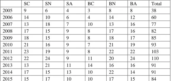
29 Size-Investment portfolios SC SN SA BC BN BA Total 2005 7 8 3 4 6 8 36 2006 5 10 6 8 7 7 43 2007 12 15 5 7 10 16 65 2008 16 23 12 15 18 19 103 2009 19 21 14 14 22 19 109 2010 19 24 17 17 24 19 120 2011 22 17 19 13 30 16 117 2012 22 25 12 15 21 24 119 2013 20 19 18 15 26 17 115 2014 18 28 15 19 21 22 123 2015 19 23 17 17 24 19 119
Table 7: Number of stocks in each one of the RHS Size-Investment portfolios each year SC SN SA MC MN MA BC BN BA Total 2005 3 6 3 6 2 4 3 4 5 36 2006 3 5 6 6 5 4 5 5 4 43 2007 11 10 1 7 6 8 4 5 13 65 2008 11 14 9 13 10 12 10 11 13 103 2009 16 13 7 8 15 14 12 9 15 109 2010 14 15 11 13 15 12 13 10 17 120 2011 18 8 13 12 15 12 9 16 14 117 2012 16 15 8 18 10 13 5 16 18 119 2013 14 10 14 14 15 10 10 14 14 115 2014 14 10 17 14 20 7 13 11 17 123 2015 13 13 13 16 14 11 10 14 15 119 Table 8: Number of stocks in each one of the LHS Size-Investment portfolios each year