NBER WORKING PAPER SERIES
FIGHT OR FLIGHT? PORTFOLIO REBALANCING BY INDIVIDUAL INVESTORS
Laurent E. Calvet
John Y. Campbell
Paolo Sodini
Working Paper 14177
http://www.nber.org/papers/w14177
NATIONAL BUREAU OF ECONOMIC RESEARCH
1050 Massachusetts Avenue
Cambridge, MA 02138
July 2008
We thank Statistics Sweden for providing the data. We received helpful comments from Markus Brunnermeier,
Ren? Garcia, David McCarthy, Stefan Nagel, Paolo Zaffaroni, three anonymous referees, and seminar
participants at Bergen, Boston University, the Federal Reserve Bank of Minneapolis, the Financial
Services Authority of the UK, Harvard University, Imperial College, MIT, Oxford University, Pompeu
Fabra, SIFR, the Stockholm School of Economics, the Swedish Financial Supervisory Authority, Universit?
Libre de Bruxelles, the University of Helsinki, the University of Venice, the Wharton School, the 2007
Brazilian Finance Society meeting in Sao Paulo, the 2007 Summer Finance Conference in Gerzensee,
the Fall 2007 NBER Asset Pricing Meeting, and the 2008 AFA meetings in New Orleans. The project
benefited from excellent research assistance by Daniel Sunesson and Sammy El-Ghazaly. This material
is based upon work supported by the Agence Nationale de la Recherche under a Chaire d?Excellence
to Calvet, BFI under a Research Grant to Sodini, the HEC Foundation, the National Science Foundation
under Grant No. 0214061 to Campbell, Riksbank, and the Wallander and Hedelius Foundation. The
views expressed herein are those of the author(s) and do not necessarily reflect the views of the National
Bureau of Economic Research.
NBER working papers are circulated for discussion and comment purposes. They have not been
peer-reviewed or been subject to the review by the NBER Board of Directors that accompanies official
NBER publications.
© 2008 by Laurent E. Calvet, John Y. Campbell, and Paolo Sodini. All rights reserved. Short sections
of text, not to exceed two paragraphs, may be quoted without explicit permission provided that full
Fight or Flight? Portfolio Rebalancing by Individual Investors
Laurent E. Calvet, John Y. Campbell, and Paolo Sodini
NBER Working Paper No. 14177
July 2008
JEL No. D14,G11
ABSTRACT
This paper investigates the dynamics of individual portfolios in a unique dataset containing the disaggregated
wealth of all households in Sweden. Between 1999 and 2002, we observe little aggregate rebalancing
in the financial portfolio of participants. These patterns conceal strong household-level evidence of
active rebalancing, which on average offsets about one half of idiosyncratic passive variations in the
risky asset share. Wealthy, educated investors with better diversified portfolios tend to rebalance more
actively. We find some evidence that households rebalance towards a higher risky share as they become
richer. We also study the decisions to trade individual assets. Households are more likely to fully sell
directly held stocks if those stocks have performed well, and more likely to exit direct stockholding
if their stock portfolios have performed well; but these relationships are much weaker for mutual funds,
a pattern which is consistent with previous research on the disposition effect among direct stockholders
and performance sensitivity among mutual fund investors. When households continue to hold individual
assets, however, they rebalance both stocks and mutual funds to offset about one sixth of the passive
variations in individual asset shares. Households rebalance primarily by adjusting purchases of risky
assets if their risky portfolios have performed poorly, and by adjusting both fund purchases and full
sales of stocks if their risky portfolios have performed well. Finally, the tendency for households to
fully sell winning stocks is weaker for wealthy investors with diversified portfolios of individual stocks.
Laurent E. Calvet
Department of Finance
Tanaka Business School
Imperial College London
London SW7 2AZ
United Kingdom
and NBER
l.calvet@imperial.ac.uk
John Y. Campbell
Morton L. and Carole S.
Olshan Professor of Economics
Department of Economics
Harvard University
Littauer Center 213
Cambridge, MA 02138
and NBER
john_campbell@harvard.edu
Paolo Sodini
Department of Finance
Stockholm School of Economics
Sveavägen 65
Box 6501
SE-113 83 Stockholm
Sweden
1. Introduction
What drives time series variations in the asset allocation of individual investors? How do households adjust their risk exposure in response to the portfolio returns that they experience? Are household portfolios characterized by inertia or high turnover? Fi-nancial theory suggests a wide range of motives for active trading and rebalancing at the household level. Realized returns onfinancial assets induce mechanical variations in portfolio allocation to which an investor is passively exposed. An investor might fight passive changes by actively rebalancing her portfolio when asset returns are expected to be time-invariant. Changes in perceived investment opportunities, on the other hand, might lead the investor to adopt aflight strategy that would amplify the decline in the share of the worst-performing assets. Furthermore, trading decisions may reflect not only asset allocation objectives, but also a disposition to hold losing and sell winning securities (Shefrin and Statman 1985; Odean 1998).
Equilibrium considerations suggest that aggregate flows from the household sec-tor provide limited and potentially misleading information on individual rebalancing. Consider for instance an economy in which households own allfinancial assets. If the aggregate value of risky securities falls, the average share of risky assets in household portfolios must necessarily fall as well. Thus, the average individual investor cannot fight aggregate variations in equity returns. When households have heterogeneous port-folios, however, there could still be substantial rebalancing at the individual level. For instance, it is an open question whether households with higher passive losses tend to buy or sell risky assets.
The empirical investigation of household rebalancing therefore requires high-quality and comprehensive micro data. Traditional datasets do not meet these requirements and have unsurprisingly led to conflicting answers on household behavior. Surveys, which have been widely used in the household finance literature, only report the allocation of household financial wealth into broad asset classes (e.g. Bilias, Georgarakos and Haliassos 2005). They permit the analysis of changes in the share of risky assets in the financial portfolio, but not the computation of active and passive changes. Thus, surveys cannot tell us whether households attempt to offset passive variations in their risky share.
Account datasets, such as 401k and brokerage accounts, present a partial view offi -nancial wealth and do not permit the computation of the risky share. Research based on discount brokerage accountsfinds evidence of intense trading activity (e.g. Odean 1999; Barber and Odean 2000), while substantial inertia is observed in 401k accounts (e.g. Agnew, Balduzzi and Sunden 2003; Ameriks and Zeldes 2004; Choi, Laibson, Madrian and Metrick 2002, 2004; Madrian and Shea 2001). These seemingly contradictory re-sults may result from a selection bias in account datasets. For example, households may
choose a discount broker precisely because they are (over)confident in their ability to process information and intend to engage in high-frequency trading. And households may trade less actively in retirement accounts than in other accounts that they control.
The Swedish dataset used in Calvet, Campbell, and Sodini (2007, henceforth “CCS 2007”) allows us to overcome these issues. We assembled data supplied by Statistics Sweden into a panel covering four years (1999-2002) and the entire country (about 4.8 million households). The information available on each resident is systematically compiled by financial institutions and corporations, and includes demographic charac-teristics, wealth portfolio, and income. Our administrative dataset is therefore more reliable than self-reported datasets, such as surveys. The wealth information is highly disaggregated and provides the worldwide assets owned by the resident at the end of a tax year. All financial assets held outside retirement accounts are reported, including bank accounts, mutual funds and stocks. However the database does not report the exact date of a sale nor information on asset purchases.
In CCS (2007) we found that household portfolios of risky assets have important idiosyncratic exposure, accounting for just over half the variance of return for the median household. While underdiversification causes only modest welfare losses for most of the population ex ante, the realized returns on household portfolios are heterogeneous ex post. In this paper we exploit this cross-sectional variation to analyze the determinants of portfolio rebalancing. The Swedish dataset is well suited for such an investigation because we can compute the risky share of every household and decompose its changes into passive and active components.
Our main results are the following. First, we study the dynamics of the risky asset share among participating households. The equal-weighted share of householdfinancial wealth invested in risky assets fell from 57% in 1999 to 45% in 2002, a decline that implies very weak active rebalancing by the Swedish household sector as a whole in response to the equity bear market of the early 2000’s. In striking contrast to this aggregate result, individual households actively rebalanced their portfolios in response to their own returns. Household-level regressions show that on average, active rebalancing compensates about one half of idiosyncratic passive variations in the risky share.
We estimate a partial adjustment model for the risky share, with heterogeneous adjustment speeds, and find that financially sophisticated households holding well di-versified portfolios adjust more rapidly towards their target risky share. We also find some evidence that the target risky share increases when households become richer, consistent with theories of declining relative risk aversion, portfolio insurance, or habit formation (Brennan and Schwartz 1988; Campbell and Cochrane 1999; Carroll 2000, 2002; Constantinides 1990; Dybvig 1995).
Second, we study patterns of entry to and exit from risky financial markets. The overall stock market participation rate increased slightly between 1999 and 2002. At
the microeconomic level, household demographics influence entry and exit as one would expect: financially sophisticated households, with greater income, wealth, and educa-tion, are more likely to enter, and less likely to exit. We are able to go beyond this familiar result to see how portfolio characteristics influence exit decisions. Wefind that households with initially more aggressive investment strategies are generally less likely to exit, although poorly diversified households and those with extremely high initial risky shares are slightly more likely to exit. If we consider mutual funds and directly held stocks as separate asset classes, we find that households are slightly more likely to exit mutual fund holding when their mutual funds have performed badly, but much more likely to exit direct stockholding when their stocks have performed well.
Third, we explore decisions to adjust positions in individual stocks and mutual funds. We begin by examining decisions to fully sell positions. We find that the absolute value of the return on a stock or fund has a positive effect on the probability that a household will sell it. This effect is much stronger for stocks with positive returns (winners) than for stocks with negative returns (losers), but the asymmetry is much weaker for mutual funds. We allow portfolio and household characteristics to influence the strength of these return effects, and find that wealthy investors with diversified portfolios of individual stocks have a weaker propensity to dispose of winning stocks and a stronger propensity to dispose of losers.
We also estimate a rebalancing model for positions that are not fully sold. Wefind that the passive change in the share of a stock or mutual fund in the risky portfolio does explain the active change, but the effect is weaker than we found when we treated all risky assets as a homogeneous asset class. Instead of a rebalancing coefficient of one half, we obtain coefficients of about one sixth which are only slightly greater for stocks than for mutual funds. Thus the difference in household decisionmaking with respect to stocks and mutual funds shows up primarily in full sales rather than in partial rebalancing decisions.
Finally, we investigate the relation between asset-level trading decisions and port-folio rebalancing. Households primarily rebalance by using a small number of trading strategies. When a household is unlucky in the sense that its risky portfolio performs worse than average, rebalancing is mostly driven by adjustments in purchases of risky assets. Conversely, when the household is lucky in the sense that its risky portfolio per-forms better than average, the household rebalances primarily by adjusting full sales of stocks and purchases of mutual funds.
Both our entry and exit results, and our results on asset-level trading decisions, are consistent with two branches of the literature. The disposition effect, that investors hold losing stocks and sell winning stocks, has been documented using account data on direct stockholdings by Odean (1998) and many others; Frazzini (2006), Goetzmann and Massa (2008), and Grinblatt and Han (2005) present evidence that this behavior
may contribute to momentum in stock returns. The literature on mutual fundflows, on the other hand,finds evidence of performance chasing by individual investors (Chevalier and Ellison 1997; Frazzini and Lamont 2007; Gruber 1996; Ippolito 1992; Ivkovic and Weisbenner 2007a; Sirri and Tufano 1998). Wefind similar patterns using different data and a different approach for classifying stocks and funds as losers or winners. Dhar and Zhu (2006) have recently found that households with higher self-reported income are less prone to the disposition effect in stock trading; our results are broadly consistent with this, although we find that wealth and portfolio diversification are more relevant than income in predicting the strength of the disposition effect.
The organization of the paper is as follows. In Section 2 we present some basic facts about the evolution of risk-taking among Swedish households in the period 1999-2002. In Section 3, we assess the magnitude of active rebalancing by decomposing household-level portfolio variations into their passive and active components. In Section 4, we estimate a partial adjustment model of portfolio risk and use it to ask which types of households adjust their portfolios more rapidly. This section also asks whether increases infinancial wealth increase households’ desired risk exposure. Section 5 explores entry and exit decisions and asset-level rebalancing in relation to the disposition effect. In Section 6, we link households’ asset-level decisions to their rebalancing strategies. Sec-tion 7 concludes. An Appendix available online (Calvet, Campbell, and Sodini 2008) presents details of data construction and estimation methodology.
2. How Has Risk-Taking Changed Over Time?
2.1. Data Description and Definitions
Swedish households pay taxes on both income and wealth. For this reason, the national Statistics Central Bureau (SCB), also known as Statistics Sweden, has a parliamentary mandate to collect highly detailed information on the finances of every household in the country. We compiled the data supplied by SCB into a panel covering four years (1999-2002) and the entire population of Sweden (about 4.8 million households). The information available on each resident can be grouped into three main categories: de-mographic characteristics, income, and disaggregated wealth.
Demographic information includes age, gender, marital status, nationality, birth-place, education, and place of residence. The household head is defined as the individ-ual with the highest income. The education variable includes high school and post-high school dummies for the household head.
Income is reported by individual source. For capital income, the database reports the income (interest, dividends) that has been earned on each bank account or each security. For labor income, the database reports gross labor income and business sector.
information. We observe the worldwide assets owned by each resident on December 31 of each year, including bank accounts, mutual funds and stocks. The information is provided for each individual account or each security referenced by its International Security Identification Number (ISIN). The database also records contributions made during the year to private pension savings, as well as debt outstanding at year end and interest paid during the year.
We will refer to the following asset classes throughout the paper. Cash consists of bank account balances and money market funds. Stocks refer to direct holdings only. Risky mutual funds are classified as either bond funds or equity funds. The latter category is broadly defined to include any fund that invests a fraction of its assets in stocks; that is, balanced funds are counted as equity funds.1 Risky assets include stocks and risky mutual funds.
Following CCS (2007), we measure a household’s totalfinancial wealth as the sum of its holdings in these asset classes, excluding from consideration illiquid assets such as real estate or consumer durables, defined contribution retirement accounts, capital insurance products that combine return guarantees with risky asset holdings, and directly held bonds. Also, our measure of wealth is gross wealth and does not subtract mortgage or other household debt. CCS (2007) summarize the relative magnitudes of all these components of Swedish household balance sheets.
A participant is a household whose financial wealth includes risky assets. In Table 1A, we report summary statistics on the assets held by participating households. To facilitate international comparisons, we convert allfinancial quantities into US dollars. Specifically, the Swedish krona traded at $0.1127 at the end of 2002, and this fixed conversion factor is used throughout the paper. The aggregate value of risky holdings declined by about one half during the bear market. Between 1999 and 2002, household stockholdings fell from $62 to $30 billion, and fund holdings from $53 to $29 billion. Cash, on the other hand, increased from $49 to $57 billion over the same period.
In the same panel we also report aggregate statistics on stock and fund holdings com-piled by the SCB and by the Swedish mutual fund association, Fondbolagens Förening (FF).2 The official statistics are incomplete because the SCB does not specifically report the aggregate cash holdings of participants and the FF series only start in 2000. The aggregate estimates obtained with our dataset closely match available official statistics. In the Appendix, we also match quite closely official aggregate statistics on flows into stocks and mutual funds. The aggregateflow into an asset class is generally quite mod-est and never exceeds a few percentage points of the total household wealth invmod-ested in
1
The managers of balanced funds periodically rebalance their holdings of cash and risky assets to maintain a stable risky share. We do not try to measure this form of rebalancing, but treat balanced funds like any other mutual funds, assuming that they have stable risk characteristics.
the class. Thus, the strong reduction in aggregate risky holdings reported in Table 1A primarily results from price movements and not from large outflows from the household sector.
Following CCS (2007), we define the following variables for each householdh. The complete portfolio contains all the stocks, mutual funds and cash owned by the house-hold. The risky portfolio contains stocks and mutual funds but excludes cash. The risky share wh,t at date t is the weight of the risky portfolio in the complete portfolio. Since the risky share is model-free, we use it extensively throughout the paper. The household’s risky portfolio is also characterized by its standard deviation σh,t, and by its systematic exposureβh,t and Sharpe ratioSh,t relative to a global equity benchmark, the MSCI World Index. The definition and estimation of these quantities are discussed in the Appendix.
The results presented in this paper are based on households that exist throughout the 1999-2002 period. We impose no constraint on the participation status of these households, but require that they satisfy the following financial requirements at the end of each year. First, disposable income must be strictly positive and the three-year rolling average must be at least 1,000 Swedish kronor ($113). Second, financial wealth must be no smaller than 3,000 kronor ($339). For computational convenience, we have selected a random panel of 100,000 households from the filtered population. Unless stated otherwise, all the results in the paper are based on this fixed subsample, and unreported work confirms the strong robustness of the reported estimates to the choice of alternative subsamples.
2.2. Cross-Sectional Dynamics of Participation and Risk-Taking
Household participation in risky asset markets increased from 61% to 65% between 1999 and 2002, as is reported in Table 1B. The inflow is equal to 20% of nonparticipating households, or about 8% of the entire population. The outflow is 7% of participants, or about 4% of the entire household population. These patterns are consistent with the “participation turnover” documented for US data (Hurst, Luoh and Stafford 1998, Vissing-Jorgensen 2002b). In Section 5, we will further investigate the microeconomic and portfolio determinants of entry and exit.
In studying rebalancing in the next two sections, we focus in each year on the large group of households that maintain participation in risky asset markets throughout the year. Between 1999 and 2002, the equal-weighted average risky share wh,t of these households fell from 57% to 45% (Table 1B). As illustrated in Figure 1A, this lower mean reflects a downward shift in the cross-sectional distribution ofwh,t, which is most pronounced in the tails.
portfolio risk. We illustrate in Figure 1B how the standard deviation of the complete portfolio, wh,tσh,t, varies with the risky share wh,t. The relation is almost linear and has similar slopes in all years. Consistent with this finding, we verify in the Appendix that the standard deviation of the risky portfolio, σh,t, has a stable cross-sectional distribution over time and is almost a flat function of the risky share.3
These results imply that Swedish households adjust their overall risk exposure pri-marily by scaling up or down their risky portfolio, passively or actively, rather by altering its composition. This justifies our emphasis on modellingwh,t in the next two sections.
3. Passive and Active Rebalancing of the Risky Share
3.1. Decomposition of the Risky Share
The change in a household’s risky share is partly determined by the household’s active trades and partly by the returns on its risky securities. For instance, the risky share tends to mechanically fall in a severe bear market. For this reason, we now decompose the change in the risky share between year tand year t+ 1, wh,t+1−wh,t,into a passive change, driven by the returns on risky assets, and an active change resulting from household rebalancing decisions. This decomposition is empirically meaningful because of the comprehensive individual asset information available in our dataset.
Thepassive risky return1+rh,t+1is the proportional change in value of a household’s
risky portfolio if the household does not trade risky assets during the year. It is easily computed from the initial risky portfolio and asset returns. Letw∗h,j,t denote the share of assetj (1≤j≤J) in the risky portfolio. If the investor does not trade between date
t and datet+ 1, the risky portfolio value att+ 1 is its value atttimes its gross return 1 +rh,t+1 =
PJ
j=1w∗h,j,t(1 +rj,t+1).We compute returnsrj,t+1 excluding dividends, as is appropriate if households consume dividends rather than reinvesting them, but we verify in the Appendix that our empirical results are essentially unchanged when dividends are included in returns.
The passive risky share is the risky share at the end of the year if the household does not trade risky assets during the year. It is a function of the initial risky share and the passive risky return:
wph,t+1 =ωp(wh,t;rh,t+1),
where
ωp(w;r)≡ w(1 +r)
w(1 +r) + (1−w)(1 +rf)
.
3Of course, the stability of average σ
h,t across risky share bins does not imply that all households own the same risky portfolio. We will indeed show in Section 3 that there is substantial heterogeneity in individual portfolio returns.
Thepassive change is the change in the risky share during the year if the household trades no risky assets during the year:
Ph,t+1 =wph,t+1−wh,t.
It is equal to zero if the investor is initially invested exclusively in cash (wh,t = 0) or exclusively in risky assets (wh,t = 1). The passive change is a hump-shaped function of the initial share if r > rf, as investors presumably expect, but a U-shaped function of the initial share if r < rf,as in our data from the bear market of 2000—2002.
The active change in the risky share, Ah,t+1 =wh,t+1−wph,t+1, is the movement in
the risky share that does not result mechanically from realized returns and thus reflects portfolio rebalancing. The total change in the risky share can be written as the sum of the active and passive changes:
wh,t+1−wh,t =Ph,t+1+Ah,t+1.
We will also use the analogous decomposition in logs:
ln(wh,t+1)−ln(wh,t) =ph,t+1+ah,t+1,
where ph,t+1 = ln(wh,tp +1)−ln(wh,t) and ah,t+1 = ln(wh,t+1)−ln(wh,tp +1) respectively
denote the active and passive changes in logs.
These decompositions treat changes in riskless asset holdings, caused by saving, dissaving, or dividends received on risky assets, as active rebalancing. An alternative approach would be to calculate the passive risky share that would result from house-hold saving or dissaving, assumed to take place through accumulation or decumulation of riskless assets, in the absence of any trades in risky assets. This alternative decom-position is attractive to the extent that households build up and run down their riskless balances for liquidity reasons that are unrelated to their investment policies. We do not pursue this alternative decomposition further here, but in our structural model of active rebalancing we do allow for a white noise error that may capture high-frequency savings effects.
3.2. Rebalancing Regressions
Changes in a household’s risky share tend to be strongly affected by the initial level of the risky share. One reason for this is purely mechanical: the total changewh,t+1−wh,t is bounded between −wh,t and 1−wh,t in the presence of short sales and leverage constraints. In addition, there may be behavioral reasons, including sluggish rebalancing and high-frequency variation in riskless balances, why the risky share may be subject to transitory shocks and gradual reversion to a long-term mean.
The scatter plots in Figure 2 show the passive, active and total changes in levels between 2001 and 2002 versus the initial risky share for a subsample of 10,000 house-holds. In panel A, the passive change is a U-shaped function of the initial share, as one expects in a bear market. Panel B reveals that the active change is close to zero for a sizeable group of households, who trade very little or not at all during the year. This observation is consistent with the inertia documented on other datasets. There is, however, considerable heterogeneity, and substantially positive or negative values of the active change are observed for many households. Moreover, the active change appears to decrease with the initial share, which suggests that the risky share tends to revert towards its cross-sectional mean. In panel C, the total change is contained in the band defined by −wh,t and 1−wh,t. The U-shaped influence of passive change is apparent, consistent with the inertia of some households. Overall, the scatter plots reveal substantial heterogeneity and strong dependence with respect to the initial risky share wh,t.
The effects of passive change and initial portfolio weight on active change are clearly visible when we group households into bins according to their initial portfolio weight, and plot the equal-weighted average within each bin of the total change, the passive change and the active change. Figure 3 shows the results for the entire 2000-2002 period (Panel A) and for each year separately (Panels B to D). Because of the bear market during our sample period, the passive change is a U-shaped function of the initial exposure
wh,t. Active rebalancing is hump-shaped and overall decreasing with the initial share, which is consistent with both mean reversion in the risky share and a tendency to offset passive changes.
In Table 2, we investigate the household-level relation between active and passive changes by estimating a rebalancing regression. We compare results in levels and in logs, but write the rebalancing regression here in logs:
ah,t+1=γ0,t+1+γ1ph,t+1+γ2(lnwh,t−lnwh,t) +uh,t+1, (3.1)
where lnwh,t denotes the equal-weighted average of the log risky share. The regressor (lnwh,t−lnwh,t) is included to capture the dependence of the active change on the initial risky share that was illustrated in Figure 2. We estimate (3.1) by OLS, both for pooled data, with year fixed effects, and for each separate cross-section. We include in the regression only households that participate both in year t and in year t+ 1. This allows us to disentangle inframarginal rebalancing from entry and exit decisions.
A fully passive household would be characterized by zero regression coefficients:
γ0,t+1 = γ1 = γ2 = 0. The estimates of γ1 are in fact close to −0.5 in the pooled regressions, and range between −0.8 and −0.4 in yearly cross-sections. Thus we find that households offset about one half of the passive change through active rebalancing. We obtain negative estimates of γ2, implying that households with a large initial risky
share have reduced their risk exposure more aggressively than other investors.
To understand the parameter estimates in Table 2 we now examine a few numer-ical examples. Consider a household invested in the value-weighted average household portfolio, with an initial share equal to the average equal-weighted share at the end of 2001: wh,t = 52.3%. In 2002, the average household portfolio yields −32.1%, and the household’s corresponding passive share is 41.7%. We infer from the pooled regression reported in Table 2A that the predicted active change equals 2.4%.
Now consider an unlucky household with the same initial share but with a realized risky return of −55.1%. Among all participants, the household is in the 5th percentile of the risky return distribution. The corresponding passive change is −20.0% and the predicted active change then equals7.1%.Alternatively, consider a lucky household with the same initial share but a realized risky return in the 95th percentile (rh,t =−7.3%). The active change is then −1.4%.Agents with returns below the cross-sectional average buy risky assets from agents with higher returns. An agent with an average share and an average return, on the other hand, makes fewer trades. The intuition that extreme agents trade more than average agents is familiar in equilibrium models.4
The rebalancing regression also predicts the effect of the initial share. For instance a household that has an initial share in the 5th percentile (wh,t = 3.9%) and owns the value-weighted average household portfolio would select an active change of 6.2%. Similarly, a household with an initial share in the 95th percentile (wh,t = 95.5%) with an average portfolio would select an active change of −10.8%. Thus, the initial share and the realized return both have substantial quantitative effects on the active change. In the online appendix (CCS 2008), we verify the robustness of the rebalancing regression by classifying households into initial risky share bins and regressing the active change onto the passive change within each bin. The estimate of the slope coefficientγ1
is strongly and significantly negative in each risky share bin, so households with high and low involvement in risky financial markets all appear to be rebalancing actively.
The rebalancing coefficient is unusually large and negative in the lowest risky share bin, particularly when we run the regression in levels. This likely results in part from a boundary effect. During the bear market, most households with low initial exposure (wh,t ≈ 0) incur small passive losses in levels, which bring them closer to the short sales constraint wh,t+1 ≥ 0. Such households may substantially increase their risky
shares, which will be associated with strongly positive active changes. Very negative active changes, on the other hand, are infeasible in levels (but are still in principle feasible in logs). The levels regression in the lowest risky share bin is therefore driven by observations with small negative passive and large positive active changes, resulting in a very negative slope coefficient γ1. The coefficient in the lowest risky share bin is 4See Calvet, Gonzalez-Eiras and Sodini (2004) for an example based on idiosyncratic nontradable risk.
somewhat less anomalous when we run the regression in logs, which encourages us to use a log specification in our subsequent analysis.
3.3. Robustness Checks
Churning. One might worry that households do not deliberately rebalance the risky share, but instead randomly buy and sell risky assets–that is, churn their portfolios. Portfolio turnover causes measurement error in the passive share, so churning biases the regression coefficient of the active change on the passive change towards−1. In this case our results tell us that there is active trading, but are not informative about deliberate rebalancing. A simple robustness check consists of confining attention to households that do not purchase new risky assets during the year. In other words, we exclude any household that has strictly positive holdings in period t+ 1 of a risky security that it did not own at all in period t. In the Appendix, we report that the corresponding rebalancing propensity is about−0.3, which is weaker than the estimates in Table 2 but still substantial.5 These estimates are conservative, since they exclude households that purchase new assets as part of an active rebalancing strategy. This analysis suggests that churning alone cannot explain the strongly negative estimates of the passive change coefficient reported in our rebalancing regressions.
Automatic Investment Plans. Automatic investment plans are another source of apparent rebalancing. Consider a household that invests a fixed monetary amount in a basket of risky assets every year, and makes no other trades. The active change is then a decreasing function of the risky portfolio’s performance, while the passive change increases with performance. Automatic investment schemes can therefore generate a negative correlation between active and passive changes.
Automatic investment plans typically imply the purchase of the same assets every year. We have already found, in our robustness check for churning, that households that purchase no new assets have a weaker rebalancing propensity, suggesting that automatic investment plans cannot be driving our results. Further, a household that only trades automatically will neither buy nor sell assets and will therefore own the same set of assets at the end of years t and t+ 1. We show in the Appendix that such households also have rebalancing propensities that are slightly lower than those reported in Table 2. It is thus very unlikely that automatic investments account for our results.
We complement this analysis with a regression on a simulated dataset of automatic savers. The automatic investment is assumed to be an exogenous percentagesof initial financial wealth.We setsequal to the average ratio in each year of savings to financial wealth for households purchasing no new assets during the year. In the Appendix, 5The appendix also estimates the adjustment model of the next section for households that purchase no new assets. The estimated adjustment speed is actually slightly higher for these households.
we regress the implied active change on the passive change and obtain only modest rebalancing propensities. Results are similar when we set s equal to a constant 3%, close to the time-series average of the yearly sratios used in our main approach.
Cash Balances. Random fluctuations in cash balances are another concern. In the next section we develop a partial adjustment model that allows high-frequency shocks to affect the target risky share. In the Appendix, we instead use a bootstrap simulation to investigate this issue. Specifically, we assume that households do not rebalance or trade risky assets during the year, and that their cash balancescbh,t follow the process:
cbh,t+1 =Rh,tcb+1cbh,t.The shocks Rcbh,t+1 are i.i.d. across households, and sampled from
the empirical cross-sectional distribution of the growth rates of cash balances. The simulation generates only modest rebalancing propensities, which shows that random fluctuations in cash balances cannot explain the rebalancing results of this section.
4. An Adjustment Model of the Risky Share
4.1. Specification
The regressions of Section 3 have shown that rebalancing is influenced by both the initial share and the passive change. This motivates us to specify a model in which households sluggishly adjust their portfolios towards a desired risky share wh,td +1.Our approach is based on three main assumptions.
First, the natural log of the observed risky sharewh,t+1 is a weighted average of the
log desired share wdh,t+1 and the log passive share wh,tp +1:
ln(wh,t+1) =φhln(wdh,t+1) + (1−φh) ln(wph,t+1) +εh,t+1. (4.1)
The errorεh,t+1is assumed to be i.i.d., resulting from measurement error, high-frequency
variations in riskless balances, and any other idiosyncratic factors influencing portfolio composition. The coefficient φh controls the household’s speed of adjustment. It can take any real value, but values between zero and one are economically most sensible. If φh = 1, the household adjusts instantaneously, and the observed share is equal to the desired share plus an error: ln(wh,t+1) = ln(wdh,t+1) +εh,t+1. A sluggish household (φh<1), on the other hand, is also sensitive to the passive share.
Second, the speed of adjustment coefficient φh is a linear function of observable characteristics:
φh=ϕ0+ϕ0xh,t, (4.2)
where the vector xh,t is independent of the errors εh,t and εh,t+1. This specification
captures the empirical relation between speed of adjustment and measures of financial sophistication such as wealth and education.
Third, the level of the log desired risky share can vary in an arbitrary manner across households, but the change in the log desired risky share is related to household characteristics by
∆ln(wh,td +1) =δ0,t+1+δ0t+1xh,t. (4.3) This equation has a convenient interpretation when households have constant relative risk aversion γh and returns on the risky asset are i.i.d. The desired risky share of household h is then wdh,t+1 = Sh,t+1/(γhσh,t+1), and changes in the log of the desired
risky share, ∆ln(wh,td +1) =∆ln(Sh,t+1/σh,t+1),are driven only by perceived variations
in investment opportunities and not by risk aversion. Equation (4.3) can then be viewed as expressing changes in perceived investment opportunities as a time-specific function of an intercept and household characteristics. This convenient property does not hold in levels, which supports our choice of a log specification. In practice, many other factors can of course alter the desired risky share, including changes in real estate holdings, human capital, background risk, or wealth if the agent has decreasing relative risk aversion.
4.2. Estimation
We now turn to the estimation of the adjustment model. In our specification, a house-hold’s target shareln(wdh,t+1)is not observed but its change∆ln(wdh,t+1)is a parametric function of characteristics (4.3). The first step is therefore to difference the portfolio share (4.1):
∆ln(wh,t+1) =φh∆ln(wdh,t+1) + (1−φh)∆ln(w p
h,t+1) +εh,t+1−εh,t.
We then substitute out φh and ∆ln(wh,td +1), using (4.2) and (4.3), and obtain the reduced-form specification:
∆ln(wh,t+1) = at+1+b0∆ln(wph,t+1) +b0xh,t∆ln(wh,tp +1)
+c0t+1xh,t+x0h,tDt+1xh,t+εh,t+1−εh,t. (4.4) The reduced-form coefficients relate as follows to the structural parameters of the ad-justment model: at+1 =ϕ0δ0,t+1, b0 = 1−ϕ0, b = −ϕ, ct+1 = δt+1ϕ0+δ0,t+1ϕ, and
Dt+1=ϕδ0t+1.
The error term of the reduced-form specification (4.4),εh,t+1−εh,t, follows a fi rst-order moving average process. A high realization of εh,tfeeds into a high sharewh,t and a high passive share wph,t+1, which implies that the errorεh,t+1−εh,t and the regressor ∆ln(wph,t+1) = lnωp(w
h,t;rh,t+1)−ln(wh,tp ) are negatively correlated. Because of this
problem, equation (4.4) cannot be consistently estimated by ordinary least squares (OLS). We handle this by finding a set of instruments that are correlated with the
explanatory variables in (4.4) but uncorrelated with the error term. The period-t+ 1 zero-rebalancing passive change
lnωp(wh,tp ;rh,t+1)−ln(wph,t)
is the passive change that would be observed att+1if the household did not rebalance at
t. Because rebalancing is limited, this variable should be positively correlated with the actual change in the passive share. At the same time, if the returnrh,t+1 is independent
of the errors, the period-t+ 1zero-rebalancing passive change is uncorrelated with εh,t and can therefore be used in a set of instruments.
In Table 3, we estimate the adjustment model for the special case where all house-holds have the same adjustment speed and target change, which corresponds to the restriction ϕ=δ = 0. The OLS regression of the total log change in the risky share on the passive log change and a timefixed effect,
∆ln(wh,t+1) =at+1+b0∆ln(wph,t+1) +uh,t+1,
gives an estimate for b0 of −0.12. This estimate is negatively biased, because the
re-gressor∆ln(wph,t+1) and the residualuh,t+1 are negatively correlated. When we correct
the bias by running instrumental variables (IV) estimation with an intercept, the log of the initial passive share, and the zero-rebalancing passive change as instruments, we obtain a considerably higher b0 estimate of0.36. The difference is economically
mean-ingful. The OLS estimate implies an adjustment speed ϕ0 = 1−b0 that is larger than
unity, while the IV estimate implies an adjustment speed ϕ0 = 0.64, which is broadly consistent with the rebalancing regressions in Section 3.
The next step is to estimate the adjustment model allowing observable household characteristics to affect the adjustment speed and the change in the desired log risky share. The set of characteristics includes demographic, financial, and portfolio charac-teristics. The first category includes age, household size, and dummies for households that have high-school education, post-high-school education, missing education data (most common among older and immigrant households), or are immigrants. The sec-ond category includes disposable income, contributions to private pension plans as a fraction of a three-year average of disposable income, log financial wealth, log real es-tate wealth, log of total debt liabilities, and dummies for households that are retired, unemployed, self-employed (“entrepreneurs”), and students. The third category, which is unique to our dataset, includes the standard deviation of the risky portfolio and the Sharpe ratio of the risky portfolio.
The inclusion of financial wealth Fht as a household characteristic creates a new difficulty. Financial wealth depends on the random cash balance observed at the end of year t, and is therefore correlated with the measurement error εh,t.A natural solution is to use as an instrument passive financial wealth Fh,t−1(1 +rch,t), where 1 +rh,tc ≡
wh,t−1(1 +rh,t) + (1−wh,t−1)(1 +rf) denotes the gross passive return on the complete portfolio. This leads us to define the following set of instruments: 1) an intercept, 2) the period-t log passive share; 3) the period-t+ 1 zero-rebalancing passive change; 4) the period-t passive financial wealth; 5) a vector of characteristics uncorrelated with the measurement error, and 6) the log passive share, zero-rebalancing passive change, passivefinancial wealth and characteristics interacted with the vector of characteristics. To simplify the estimation of the full model (4.4), given that we have a short panel with only two years of data after differencing, we estimate the reduced form assuming constant coefficients over time on the household characteristics: ct+1 =c, andDt+1 =D.
The structural restrictions of the model then imply that the time fixed effectsat+1 are
also constant, as are the structural coefficients in the equation for the change in the desired risky share, (4.3): δ0,t+1 =δ0 and δt+1 =δ. We do not impose constant time fixed effects, butfind them to be almost identical in 2001 and 2002.
IV estimates of this model are reported in thefirst set of columns of Table 4. Each characteristic is standardized to have zero cross-sectional mean. We also normalize to unity the cross-sectional standard deviation of each continuous characteristic, so the reported regression coefficient reveals the effect of a one-standard-deviation change in the characteristic. To keep the table at a manageable size, we only report the structural vectors ϕ and δ of the full regression. The median value of the speed parameter is 0.73 and the average log target change is -0.18 in 2002. These numbers are consistent with the rebalancing regressions in Section 3 and imply a modest revision in the target share. The estimates of ϕandδ are robust to the inclusion or exclusion of the nonlinear interacted termx0h,tDxh,t.
The most striking result in Table 4 is that the speed of adjustment tends to increase with variables associated with financial sophistication, such as education, disposable income, debt, and financial and real estate wealth. In addition, households with well diversified portfolios (high Sharpe ratios) have higher adjustment speeds. Entrepreneur-ial activity, retirement, unemployment, and household size, on the other hand, reduce the adjustment speed.
Changes in the target risky share are less consistently related to household char-acteristics. Households with greater financial wealth reduce their target less. Real estate wealth, on the other hand, works in the opposite direction, perhaps because the booming Swedish real estate market reduced the attractiveness of stocks to real-estate-oriented investors in 2001 and 2002. Well diversified and aggressive households, with higher Sharpe ratios and riskier portfolios, reduce their target share more; but so do larger, older, and immigrant households that normally invest cautiously (CCS 2007).
The estimates in Table 4 can be used to compute the predicted speed parameter and target change of every household. The cross-sectional distribution of the speed φh
numbers which seem quite reasonable. Similarly, the target change ∆ln(wdh,t+1) has a 5th percentile of -29%, a median value of -18%, and a 95th percentile of 5%, which again seem quite reasonable in a severe bear market.
In the appendix, we report the average characteristic values for households at dif-ferent percentiles of the predicted adjustment speed and target change distributions. The average household at the 5th percentile of adjustment speed has disposable income of about $20,700 and wealth of $10,500, 47% of which is invested in risky assets with a Sharpe ratio of 0.22. 35% of these slowly adjusting households have a high school education, and 6% have a college education. At the 95th percentile of adjustment speed, by contrast, the average household has disposable income of $42,800 and wealth of $56,200, 70% of which is invested in risky assets with a Sharpe ratio of 0.31. 95% of these rapidly adjusting households have a high school education, and 71% have a college education. In short, rapidly adjusting households appear to be morefinancially sophisticated than slowly adjusting households.
The appendix also reports results when we estimate the adjustment model separately for the years 2001 and 2002, allowing both adjustment speeds and target changes to vary across years. The results are qualitatively similar to those reported in Table 4, although adjustment speeds appear to be faster in 2001 than in 2002, and some of the individual characteristics have coefficients that are unstable over time.
4.3. Impact of Wealth Changes on Risk-Taking
In the first set of columns of Table 4, we have used slowly evolving demographic and financial variables as household characteristics that may influence portfolio ad-justment. We now explore the possibility that portfolio decisions are also affected by high-frequency variation in financial wealth. Several branches of financial theory sug-gest that an increase in financial wealth might increase the propensity to take risk. In the presence of borrowing constraints, individuals become less risk-averse as they be-come richer and thus less likely to face a binding constraint in the future. Even in the absence of such frictions, investors with decreasing relative risk aversion tend to hold a higher risky share as their wealth goes up. Carroll (2000, 2002) builds such a utility function, and documents a positive empirical relation between household wealth and the risky share. Models of portfolio insurance (Brennan and Schwartz 1988) and habit formation (Constantinides 1990, Dybvig 1995, Campbell and Cochrane 1999) also imply a positive relation between wealth and the risky share, because richer agents are more willing to take risk as their wealth moves further above the minimum level required by the portfolio insurance policy or the present value of the future habit.
In the second set of columns of Table 4, we reestimate the adjustment model using the contemporaneous change in logfinancial wealth as an additional household characteristic
that can affect the change in the target. We add one instrument to the previous set, the zero-rebalancing return on the complete portfolio, that is, the return that each household would earn at t+ 1 if it did not rebalance at t. We find that an increase in log financial wealth leads to a higher target risky share, while the impact of other characteristics is largely unchanged.
In the Appendix, we show that results are similar when we estimate the model separately for the years 2001 and 2002, although the effect of the change in log fi nan-cial wealth on the target risky share is stronger in 2002. The Appendix also reports similar results when we allow the change in log financial wealth to affect the adjust-ment speed as well as the desired risky share. We find little variation in the change in log financial wealth across rapidly adjusting and slowly adjusting households, but large variation across households with high and low predicted changes in the target risky share. Households at the 5th percentile of the target change experience average financial wealth declines of 44%, while households at the 95th percentile of the target change experience average financial wealth increases of 31%.
In a recent study, Brunnermeier and Nagel (2007) assess the empirical relation be-tween wealth and the risky share using US data from the Panel Study of Income Dy-namics (PSID). They regress the change in the risky share (in levels) on the change in financial wealth (in logs) and control variables, and obtain a small and slightly negative wealth coefficient. They attribute this result to inertia. When a household saves in the form of cash during the year and only partially rebalances its financial portfolio, its risky share tends to fall mechanically.
In the Appendix, we estimate the Brunnermeier-Nagel regression on our Swedish dataset. The OLS estimate of the regression coefficient is slightly negative, consistent with Brunnermeier and Nagel’s finding; but it becomes positive when we estimate the regression by instrumental variables. Similarly, we find a positive relation between the change in the risky share and the lagged change in financial wealth. These results are robust to separate estimation of the regression in the years 2001 and 2002. Thus, controlling for endogeneity problems and household inertia, the Swedish data do show some evidence for a positive link between wealth changes and risk-taking.
4.4. Connection with Rebalancing Regressions
The adjustment model of this section is intimately related to the rebalancing regressions we estimated in section 3. When the adjustment speed and target changes are the same for all households, the adjustment model implies:
ah,t+1 =φδ0,t+1−φph,t+1−φ(lnwh,t−lnwdh,t) +εh,t+1, (4.5)
which is analogous but not exactly identical to the rebalancing regression (3.1). The similarity suggests that the adjustment speed should be close to the regression coeffi
-cients reported in Table 2B; this is indeed the case in our empirical results since the median speedφh and the linear regression coefficient−γ1 are both about one half. The distance to the target, lnwh,t−lnwdh,t,represents the only difference between (3.1) and (4.5). We can therefore view (3.1) as a reduced-form specification in which all house-holds have the same speed of adjustment and the distance to the target,lnwh,t−lnwdh,t, is proxied by a rescaled distance to the cross-sectional mean, λ(lnwh,t−lnwh,t).
We show in the Appendix that the adjustment model with heterogeneous agents leads to additional terms in the rebalancing regressions. Section 4 thus improves on the specification in Section 3 by: (1) providing more precise micro foundations; (2) correctly estimating the structural parameters even though the target is unobserved; and (3) allowing for heterogeneity in the adjustment speed and the target change.
In the Appendix, we investigate the role of household characteristics in the rebalanc-ing regression (3.1). The reduction in the risky share is in all years less pronounced for households with higherfinancial wealth or debt. These households were more willing to maintain their proportional investments in risky assets than were other Swedish house-holds. We interact demographic variables with passive changes, andfind that wealthier and more sophisticated households tend to have more negative regression coefficients of active changes on passive changes; that is, they rebalance more actively. Thesefindings confirm the results of the adjustment model. They are limited, however, in that they do not allow us to disentangle household inertia from changes in the target risky share, as the adjustment model can do.
5. Asset-Class Participation, Asset-Level Rebalancing, and the
Dispo-sition E
ff
ect
We now study household decisions to participate in asset classes (risky assets, mutual funds, and direct stockholding) and to rebalance positions in individual assets. We relate these decisions to the disposition effect, the tendency to realize gains and hold on to losses, where gains and losses are measured relative to the asset’s purchase price. The disposition effect was identified by Shefrin and Statman (1985) and has been widely documented (e.g. Odean 1998).
The Swedish dataset unfortunately does not provide the date or price of individual asset trades. For this reason, we use an asset’s return during the year as an alterna-tive measure of performance. This implies that we are assessing the robustness of the disposition effect to this alternative benchmark. The Swedish dataset has an impor-tant compensating advantage: we can relate the disposition effect to demographic and financial characteristics of households, as well as the characteristics of the portfolios they hold. This allows us to extend the recent finding of Dhar and Zhu (2006) that households with higher self-reported income are less prone to the disposition effect.
5.1. Entry and Exit at the Risky Portfolio and Asset Class Levels
We begin by investigating the probability that a household enters or exits risky asset markets. In Table 5, we run pooled probit regressions of the form yh,t=Φ(x0h,tγ+γ0,t), where yh,t denotes participation status, xh,t is the vector of characteristics, and γ0,t is a time-dependent intercept. The time interval is annual, and we pool data from 2000, 2001, and 2002. To facilitate comparison, we report in the last three rows the rates of entry to and exit from risky asset markets in each year.
In the first set of three columns, we analyze the probability that a nonparticipant in year t holds risky assets in year t+ 1. Thefirst two columns report coefficients and t-statistics, while the third column assesses the economic magnitude of the coefficient estimates by reporting the impact on the entry probability of increasing a non-dummy regressor by one standard deviation, or setting a dummy variable equal to one. This impact depends on the base rate of entry; we report it for the year 2001, in which the overall entry rate was 5.7%, much lower than the rate in 2000 and slightly greater than the rate in 2002.
The probability of entry increases with standard measures offinancial sophistication such as education, financial and real estate wealth, and the private pension savings rate. Conversely, the exit probability decreases with variables associated with investor sophistication, as shown in the middle three columns of Table 5. The entry and exit regressions are thus remarkably symmetric and consistent with earlier research on cross-sectional data. Household characteristics that predict participation in a cross-section (e.g. Guiso, Haliassos, and Jappelli 2002, CCS 2007) also help to explain entry and exit in the panel.
In the last three columns of Table 5, we investigate how the exit probability is affected by portfolio characteristics. The exit probability decreases with the initial risky share and the standard deviation of the risky portfolio. More aggressive agents have higher risk-tolerance and are less likely to entirely give up the benefits offinancial risktaking. A complementary explanation is that households sluggishly adjust their portfolios, as in Section 4; more aggressive investors are then more reluctant to dispose of all their risky assets. The exit probability, however, increases with extreme risk-taking, as measured by a dummy equal to unity if the risky share exceeds ninetyfive percent. Extreme risk-takers presumably have limited understanding of financial risk and may be prone to panic selling in a bear market.
A household is also more likely to exit if it is undiversified (low Sharpe ratioSh,t). Fi-nally, we consider the performance of the risky portfolio during the year, and distinguish between positive returns (winning portfolios) and negative returns (losing portfolios). Large absolute returns tend to increase the probability of exit, and the effect is slightly more pronounced for winners than losers.
We next investigate the separate roles of direct stock and mutual fund holdings. It is useful to decompose the overall Sharpe ratio into its stock and fund components. Let
Dh,t denote the share of direct stockholdings in the risky portfolio, SD,h,t and SF,h,t the Sharpe ratios of the stock and fund portfolios, and σD,h,t and σF,h,t their standard deviations. The Sharpe ratio of the risky portfolio satisfies:
Sh,t=CD,h,t+CF,h,t,
where the components of the Sharpe ratio attributable to each asset class are given by
CD,h,t = SD,h,t Dh,tσD,h,t σh,t , CF,h,t = SF,h,t (1−Dh,t)σF,h,t σh,t .
The contribution of an asset class to the overall Sharpe ratio is large if the household holds a diversified portfolio of assets in the class, which represents a large fraction of its risk exposure.
In Table 6, we investigate exit decisions by asset class for a subset of households that initially own both stocks and mutual funds. As in the previous tables, we include financial and demographic variables and the risky portfolio’s standard deviation. We also consider the contributions of stocks and funds to the overall Sharpe ratio and the performance during the year of the household’s stocks and funds. These variables are used to explain the probability that a participating household disposes of all its risky assets (first three columns), all its directly held stocks (next three columns) or all its mutual funds (last three columns).
Most of the patterns in Table 6 are consistent with those already shown in Table 5. The striking new result in Table 6 is that the exit probability from risky asset markets increases strongly with the performance of winning stock portfolios. Winning stock portfolio performance has an even greater impact on the probability of exiting direct stockholding, as shown in the second column of the table. Thesefindings are consistent with the disposition effect on direct stockholdings: the owner of a winning stock portfolio is more likely to sell it and leavefinancial markets. There is little evidence in the table of a comparable disposition effect for mutual funds. The owner of a winning mutual fund portfolio is slightly more likely to liquidate it, but the effect is small and statistically insignificant; losses have a larger effect on the mutual fund sales probability, consistent with the literature on performance-sensitivity of mutual fund holdings (Chevalier and Ellison 1997; Frazzini and Lamont 2007; Gruber 1996; Ippolito 1992; Sirri and Tufano 1998; Ivkovic and Weisbenner 2007a).
5.2. Dynamics of Individual Asset Shares
We now investigate how a household adjusts during year t+ 1 the asset positions that it holds at the end of yeart. Since exit decisions have been addressed in Section 5.1, we consider only households that own risky assets in both years. Also, we confine attention to assets which are held at the end of yeart and do not attempt to model household decisions to purchase new assets.
A household owning a stock at the end of 2000 had, by the end of 2001, partially sold it with probability 27%, fully sold it with probability 16%, held on to it with probability 22%, and bought additional units of the same stock with probability 35%. Partial sales and partial purchases are thus more frequent than full sales or continued holdings. As reported in the Appendix, this property holds in all years and is even more pronounced for mutual funds: the probability of a fund’s full sale is less than 10% while the probability of a partial purchase is about 60%. The high probability of partial purchases for funds is attributable in part to the dividend reinvestment plans offered by most investment companies. Even though full sales are a relatively limited phenomenon, we begin by studying them separately given their importance in the disposition effect literature.
Full Sales. In Table 7, we analyze the probability that a household owning a risky assetj at datethas fully disposed of it by the end of yeart+ 1. The regression distin-guishes between stocks and funds, and between assets with positive returns (winners) and negative returns (losers) during the year. We include household demographic and financial characteristics, and portfolio characteristics, both directly and interacted with the return on the asset during the year.6 The table reports the coefficients on the char-acteristics interacted with return but omits the direct coefficients; the full regression is reported in the Appendix.
The probability of fully selling an asset increases with the absolute value of its performance during the year. Households are more likely to fully sell extreme losers or extreme winners than stocks and funds that have close to zero returns. For stocks, this effect is much more pronounced for winners than for losers, which seems consistent with a disposition effect on direct stockholdings. For funds, performance also impacts the probability of a full sale, but there is substantially less asymmetry between losers and winners. The tendency to sell losing funds is consistent with the literature on performance sensitivity. For winning funds, however, household behavior is both driven by the tendency to hold on to winners, for instance because they are run by skilled managers, but also a tendency to sell winning assets in order to rebalance the risky 6In Table 7, we assign a value of zero to the characteristic of an asset class if the household has no investments in this class. A similar convention is used in the remainder of the section.
portfolio. The connection between asset trades and portfolio rebalancing will be further investigated in section 6.
Financial and portfolio characteristics have a substantial impact on the probability of a full sale of stock. Wealthier households with riskier overall portfolios and better diversified stock portfolios are less likely to sell a winning stock but more likely to sell a losing stock. These effects reduce the asymmetry between winners and losers and therefore weaken the disposition effect on direct stockholdings. Losing funds are also more likely to be sold by wealthier households, but we otherwise find little significance of characteristics in the regressions that predict full sales of mutual funds.
Overall, the table reveals that more sophisticated and aggressive households, with larger portfolios of directly held stocks, appear to be less prone to the disposition effect.
Partial Sales, Continued Holdings and Partial Purchases. We have shown in previous sections that householdsfight idiosyncratic passive variations in the risky share. We now investigate whether they also rebalance individual security positions in the risky portfolio. The analysis excludes full sales, but considers partial sales, continued holdings and partial purchases. In the Appendix, we check that the evidence of asset-level rebalancing is even stronger when we include full sales.
For each householdh, we definew∗
h,j,t as the share of asset j in the risky (not the complete) portfolio at the end of periodt,rh,t+1 as the net return on the risky portfolio
between tand t+ 1, and rj,t+1 as the net return on assetj. If the household does not
trade risky assets in the next period, the asset’s passive share at the end of t+ 1is:
w∗h,j,tp +1 =w∗h,j,t1 +rj,t+1 1 +rh,t+1 . LetA∗ h,j,t+1 =w∗h,j,t+1−w∗ p h,j,t+1andPh,j,t∗ +1=w∗ p
h,j,t+1−w∗h,j,tdenote the corresponding active and passive changes in levels, and a∗h,j,t+1 and p∗h,j,t+1 their equivalents in logs.
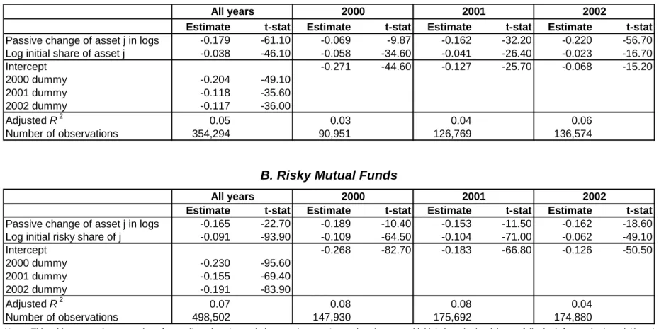
We estimate a rebalancing model for individual assets. In Table 8, we report the pooled and yearly regressions of the log active change a∗
h,j,t+1 on the initial share and
the log passive change p∗h,j,t+1, both for stocks (panel A) and funds (panel B). The rebalancing coefficient is only slightly more negative for stocks than for funds, and approximately equal to one sixth. Thus, when we focus on partial sales, the rebalancing coefficient is roughly constant across funds and stocks. In the Appendix, we report the rebalancing regressions in levels, and alsofind evidence of active rebalancing at the asset level. The rebalancing coefficients in levels are somewhat larger in absolute value, but also more variable across regressions.
The interpretation of Table 8 is complicated by the ambiguous predictions of fi -nancial theory. In a mean-variance portfolio choice problem with constant investment opportunities, the optimal weights of individual assets in the risky portfolio are time-invariant, which implies complete rebalancing with A∗
rebalancing might be justified by a variety of factors such as changes in risk and return expectations, taxes, transactions costs, or Bayesian updating of beliefs about mutual fund management. In the Appendix, we ask how the propensity to rebalance individual assets varies with household and portfolio characteristics, but do not find any strong effects.
In this section we have shown that households are much more likely to fully sell a stock when it has performed well, and slightly more likely to sell a losing fund. Thisfi nd-ing is consistent with the literature on the disposition effect. If a household continues to own a stock or mutual fund, however, its behavior is well described by a rebalancing model with a rebalancing coefficient of about one sixth, and the rebalancing propensity is almost the same for stocks and for mutual funds.
6. Trading Decisions and Risky Portfolio Rebalancing
We now investigate how rebalancing of the complete portfolio, which was documented in Sections 3 and 4, relates to the dynamics of individual asset holdings discussed in Section 5. We focus on the contribution of different asset classes and transaction types to the overall active change of the risky share.
The active change of the risky share between dates t and t+ 1 can be decomposed as
Ah,t+1 = X
j
(wh,j,t+1−wh,j,tp +1), (6.1)
where wh,j,t+1 denotes the share of assetj in the complete portfolio at the end of year
t+ 1,and wph,j,t+1 is the passive share of asset j in the complete portfolio if the agent does not trade during the year:
wh,j,tp +1= wh,j,t(1 +rj,t+1)
wh,t(1 +rh,t) + (1−wh,t)(1 +rf)
.
The individual terms on the right hand side of (6.1) can be grouped into specific asset classes c(fund or stock) and transaction types θ(purchase or sale):
Ah,t+1 = X
c,θ
Ah,c,θ,t+1.
We can also distinguish between partial sales, full sales, partial purchases (assets already held by the household), and full purchases (new types of assets).
Each component of the active change Ah,c,θ,t+1 can be regressed on the passive
change of the risky portfolio Ph,t+1, the demeaned initial risky share wh,t−w¯h,t, and a time-dependent intercept. The corresponding rebalancing coefficients γ1,c,θ,t+1 add up to the overall rebalancing coefficient: Pθ,cγθ1,c,t+1 =γ1.This decomposition allows
us to identify how various asset classes and transaction types contribute to portfolio rebalancing.
Given our findings in Section 4 on the disposition effect, it is also useful to distin-guish between transactions carried out bylucky andunlucky households. Specifically, a household is classified as lucky if the return on its risky portfolio exceeds the population average during the same year. In Table 9, we report the rebalancing coefficientsγθ1,c,t+1
and their t-statistics, and refer the reader to the appendix for the full regression re-sults. Lucky and unlucky households both have a rebalancing coefficient of about−0.5, which is slightly larger in absolute value for lucky households. Stocks and funds play an important role in rebalancing for both groups of investors. We have verified that our results are almost identical when the median return is used as an alternative cutoff, or when we consider households in the top third and bottom third of risky portfolio performance.
When we disaggregate sales and purchases, however, we do see important differences between lucky and unlucky households. Lucky households rebalance primarily by ad-justing their stock sales and fund purchases. The rebalancing coefficient of −0.58 is almost entirely explained by the coefficients of full sales (-0.29) and partial purchases (-0.24). That is, lucky households, who need to reduce their holdings of risky assets, achieve this objective by fully selling more stocks and buying less mutual funds than they would otherwise.
Unlucky households, on the other hand, mainly rebalance by adjusting their pur-chases of new assets. The rebalancing coefficient (equal to -0.50) is primarily driven by stock purchases (-0.30) and fund purchases (-0.13). The impact of asset sales is marginal. Households thus primarily rebalance by increasing their (full) stock sales and reduc-ing their fund purchases when they are lucky, and increasreduc-ing their purchases of risky assets (primarily stocks) when they are unlucky. These common strategies minimize transaction costs. The exception is the full sale of stocks by lucky households, which may be caused by the disposition effect.
In the Appendix, we investigate how these common rebalancing strategies are in-fluenced by household characteristics. We find that wealthier households with more diversified portfolios tend to rebalance more strongly through purchases of risky assets but less through stock sales. Thus, it appears that more sophisticated households are less pro