Transform Analysis and Asset Pricing for Affine Jump-Diffusions

NBER WORKING PAPER SERIES

TRANSFORM ANALYSIS AND ASSET PRICING FOR AFFINE

JUMP-DIFFUSIONS Darrell Duffie Jun Pan Kenneth Singleton Working Paper 7105 http://www.nber.org/papers/w7105

NATIONAL BUREAU OF ECONOMIC RESEARCH 1050 Massachusetts Avenue

Cambridge, MA 02138 April 1999

We are grateful for extensive discussions with Jun Liu; conversations with Jean Jacod, Monika Piazzesi, Philip Protter, and Ruth Williams; and support from the Financial Research Initiative, The Stanford Program in Finance, and the Gifford Fong Associates Fund, at the Graduate School of Business, Stanford University. The views expressed herein are those of the authors and do not necessarily reflect the views of the National Bureau of Economic Research.

© _{1999by Darrell Duffie, Jun Pan, and Kenneth Singleton. All rights reserved. Short sections of text, not} to exceed two paragraphs, may be quoted without explicit permission provided that full credit, including

Transform Analysis and Asset Pricing for Affine Jump-Diffusions

Darrell Duffie, Jun Pan, and Kenneth Singleton NBER Working Paper No. 7105

April 1999

JELNo. Gi

ABSTRACT

In the setting of "affine" jump-diffusion state processes, this paper provides an analytical treatment of a class of transforms, including various Laplace and Fourier transforms as special cases, that allow an analytical treatment of a range of valuation and econometric problems. Example applications include fixed-income pricing models, with a role for intensity-based models of default, as well as a wide range of option-pricing applications. An illustrative example examines the

implications of stochastic volatility and jumps for option valuation. This example highlights the impact on option 'smirks' of the joint distribution ofjumps in volatility and jumps in the underlying asset price, through both amplitude as well as jump timing.

Darrell Duffie Jun Pan

Graduate School of Business Graduate School of Business

Stanford University Stanford University

Stanford, CA 93405 Stanford, CA 93405

[email protected] [email protected]

Kenneth Singleton

Graduate School of Business Stanford University

Stanford, CA 93405 and NBER

1 Introduction

In valuing financial securities in an arbitrage-free environment, one inevitably

faces a trade-off between the analytical and computational tractability of

pricing and estimation, and the complexity of the probability model for the

state vector X. In the light of this trade-off, academics and practitioners

alike have found it convenient to impose sufficient structure on the condi-tional distribution of X to give closed- or nearly closed-form expressions for securities prices. An assumption that has proved to be particularly fruitful in developing tractable, dynamic asset pricing models is that X follows an affine jump-diffusion (AJD), which is, roughly speaking, a jump-diffusion process for which the drift vector, "instantaneous" covariance matrix, and jump intensities all have affine dependence on the state vector. Prominent

among AJD models in the term-structure literature are the Gaussian and

square-root diffusion models of Vasicek [1977] and Cox, Ingersoll, and Ross

[1985]. In the case of option pricing, there is a substantial literature building on the particular affine stochastic-volatility model for currency and equity

prices proposed by Heston [1993].

This paper synthesizes and significantly extends the extant literature on affine asset pricing models by deriving a closed-form expression for an "ex-tended transform" of an AJD process X, and then showing that this

trans-form leads to analytically tractable pricing relations for a wide variety of valuation problems. More precisely, fixing the current date t and a future payoff date T, suppose that the stochastic "discount rate" R(X), for

com-puting present values of future cash flows, is an affine function of X. Also,

consider the generalized terminal payoff function (vo + v1 XT) euX(T) of XT,

where _{v0 is scalar and the n elements of each of the v1 and u are scalars.}

These scalars may be real, or more generally, complex. We derive a closed-form expression for the transclosed-form

E (exp (_

1T

R(X8, s) ds) (v0 + v1 XT) eT),

(1.1)

where E denotes expectation conditioned on the history of X up to t. Then, using this transform, we show that the tractability offered by extant,

special-ized affine pricing models extends to the entire family of AJDs. Additionally, by selectively choosing the payoff (v0+v1 .XT) e'(T), we significantly extend

with X following an AJD. To motivate the usefulness of our extended

trans-form in theoretical and empirical analyses of affine models, we briefly outline

three applications.

1.1 Affine, Defaultable Term Structure Models

There is a large literature on the term structure of default-free bond yields that presumes that the state vector underlying interest rate movements

fol-lows an AJD (see, e.g., Dai and Singleton [1999] and the references therein).

Assuming that the instantaneous riskless short-term rate Tt is an affine

func-tion of an n-dimensional AJD process X (that is Tt =_{Po + ,oi X) ]Duffie}

and Kan [1996] show that the (T —_{t)-period zero-coupon bond price,}

E (exp (JT))

(1.2)

is known in closed form, where expectations are computed under the

risk-neutral measure.1

Recently, considerable attention has been focused on extending these models to allow for the possibility of default in order to price corporate

bonds and other credit-sensitive instruments.2 To illustrate the new pricing

issues that may arise with the possibility of default, suppose that default is governed by a stochastic intensity A and that, upon default, the holder recovers a constant fraction w of face value. Then, from results in Lando

[1998], the price of a (T —_{t)-periodzero-coupon bond is given under}

techni-cal integrability conditions by

E (exp (_

f(rs

+ A8) ds)) + w f

E

(s

exp

(

f8( +

A) du)) ds.

(1.3)

The first term in (1.3) is the value of a claim that pays $1 contingent on

survival to maturity T, while the second term is the value of the claim that pays w at date s should the issuer default at that date, and nothing otherwise.

Both the first term and, for each s, the expectation in the second term

can be computed in closed form using our extended transform. Specifically,

1The entire class of affine term structure models is obtained as the special case of (1.1) found by setting R =_r,u =0,vo =1, and v1 =0.

assuming that both rt and

are affine in an AJD process X, the first

expectation in (1.3) is the special case of (1.1) that is obtained by letting

R(X, t) =

Tt

+ )t, u =

0, v0 1 and v1 =0. Similarly, each expectation in

(1.3) of the form E (A8 exp (—

f8 r,

+ )' du)) is obtained as a special case

of (1.1) by setting u = 0,

R(X, t) =

Tt

+ At, and v0 + v1 X =

A. Thus,

using our extended transform, the pricing of defaultable zero-coupon bonds

with constant fractional recovery of par reduces to the computation of a

one-dimensional integral of a known function. Similar reasoning can be used

to derive closed-form expressions for zero prices in environments where the default arrival intensity is affine in X, and there is "gapping" risk associated

with unpredictable transitions to different credit categories (see Lando [1998]

for the case of w = _0).

A different application of the extended transform is pursued by Piazzesi [1998] who extends the AJD model in order to treat term-structure models with releases of macro-economic information and with central-bank

interest-rate targeting. She considers jumps at both random and at deterministic

times, and allows for an intensity process and interest-rate process that have linear-quadratic dependence on the underlying state vector, extending the basic results of this paper.

1.2 Estimation of Affine Asset Pricing Models

Another useful implication of (1.1) is that, by setting R =_0, v0 = 1, and

v1 =_0, we obtain a closed-form expression for the conditional characteristic

function of XT given X, defined by

X, t, T) E (eT X) .

Because knowledge of is equivalent to knowledge of the joint conditional density function of XT, this result is useful in estimation and all other applications involving the transition densities of an AJD.

For instance, Singleton [1998] exploits knowledge of to derive maximum likelihood estimators for AJDS based on the conditional density of X1 given X, obtained by Fourier inversion of

f(Xt+iXt;7) — _N

f

e_1(u,Xt,t,t

_{+ 1) du. (1.4)}

(2ir) a

Das [1998] exploits (1.4) for the specific case of a Poisson-Gaussian AJD to compute method-of-moments estimators of a model of interest rates.

of the conditional characteristic function. By definition, t satisfies

PJ [c+' —

(u,

X, t, t + 1)] = 0, (1.5)

so any measurable function of X is orthogonal to the "error" (emflXt+1 c5(u,Xt,t,t + 1)). Singleton [1998] uses this fact, together with the known functional form of to construct generalized method-of-moments estimators of the parameters governing AJDs and, more generally, the parameters of asset pricing models in which the state follows an AJD. These estimators are computationally tractable and, in some cases, achieve the same asymptotic

efficiency as the maximum likelihood estimator.3

1.3 Affine Option Pricing Models

In an influential paper in the option-pricing literature, Heston [1993] showed

that the risk-neutral exercise probabilities appearing in the call option pricing

formulas for bonds, currencies, and equities can be computed by Fourier in-version of the conditional characteristic function, which he showed is known in closed form for his particular affine, stochastic volatility model. Build-ing on this insight,4 a variety of option-pricBuild-ing models have been developed

for state vectors having at most a single jump type (in the asset return),

and whose behavior between jumps is that of a Gaussian or "square-root"

diffusion .

Knowingthe extended transform (1.1) in closed-form, we can extend this

option pricing literature to the case of general multi-dimensional AJD pro-cesses with much richer dynamic inter-relations among the state variables

and much richer jump distributions. For example, we provide an analyti-cally tractable method for ricing derivatives with payoffs at a future time

T of the form (e(T) —

_c) , where c is a constant strike price, b E R', X

3Liu and Pan [1997] and Liu [1997] propose alternative estimation strategies that exploit

the special structure of affine diffusion models.

4Among the many recent papers examining option prices for the case of state variables following square-root diffusions are Bakshi, Cao, and Chen [1997], Bakshi and Madan [1999], Bates [1996], Bates [1997], Chen and Scott [1993], Chernov and Ghysels [1998], Pan [1998], Scott [1996], and Scott [1997], among others.

5More precisely, the short-term interest rate has been assumed to be an affine function of

independent square-root diffusions and, in the case of equity and currency option pricing, spot-market returns have been assumed to follow stochastic-volatility models in which volatility processes are independent "square-root" diffusions that may be correlated with the spot-market return shock.

is an AJD, and y max(y, 0). This leads directly to pricing formulas for

plain-vanilla options on currencies and equities, quanto options (such as an

option on a common stock or bond struck in a different currency), options on

zero-coupon bonds, caps, floors, chooser options, and other related

deriva-tives. Furthermore, we can price payoffs of the form (b X(T) — c)+ and

X(T) and this allows us to price "slope-of-the-yield-curve" options and certain Asian options.6

In order to visualize our approach to option pricing, consider the price p at date 0 of a call option with payoff (edX(T) — at date T, for given

d e

11 and strike c, where X is an n-dimensional AJD, with a short-term

interest-rate process that is itself affine in X. For any real number y and any

a and b in ,

let Ca,b(Y) denote the price of a security that pays ea(T) at

time T in the event that b X(T) < y. As the call option is in the money

when —d• X(T) < — lnc, and in that case pays e(X(T) —ceOX(T), we have

the option priced at

p Gd,_d(—lnc)

— cGo,_d(—lnc). _(1.6) Thus, it is enough to be able to compute the Fourier transform a,b(•) of

Ga,b() (treated as a measure), defined by

+

ga,b(z)

f e1

dGa,b(Y),

for then well-known Fourier-inversion methods can be used to compute terms of the form Ca,b(Y) in (1.6).

There are many cases in which the Fourier transform ca,b(.)of_{Ga,b() can} be computed explicitly. We extend the range of solutions for the transform

a,b()

from those already in the literature to include the entire class of

AJDs by noting that ga,b(z) is given by (1.1), for the complex coefficient

vector u =

a _{+ izb, with v0 =} 1 and v1 = 0. _{This, because of the affine}

structure, implies under regularity conditions, that

ca,b(z)

= e0)0)X(0),

(1.7)

6j

a_{complementary analysis of derivative security valuation, Bakshi and Madan [1999]}

show that knowledge of the special case of (1.1) with v0 +v1 •XT =1is sufficient to recover

the prices of standard call options, but they do not provide explicit guidance as to how to compute this transform. Their applications to Asian and other options presumes that the state vector follows square-root or Heston-like stochastic-volatility models for which the relevant transforms had already been known in closed form.

where and 3 solve known, complex-valued ordinary differential equations

(ODEs) with boundary conditions at T determined by z. In some cases,

these ODEs have explicit solutions. These include independent square-root

diffusion models for the short-rate process, as in Chen and Scott [1995],

and the stochastic-volatility models of asset prices studied by Bates [1997]

and Bakshi, Cao, and Chen [1997]. Using our ODE-based approach, we

derive other explicit examples, for instance stochastic-volatility models with

correlated jumps in both returns and volatility. In other cases, one can

easily solve the ODEs for c and / numerically, even for high-dimensional

applications.

Similar transform analysis provides a price for an option with a payoff of the form (d. XT —

c),

again for the general AJD setting. For this case, we provide in Appendix E an equally tractable method for computing the

Fourier transform of Ga,b,d( _{), where} Ga,b,d(y) is the price of a security that

pays e(T)a .

X(T)

at T in the event that b .

X(T)

<

y. This transform

is again of the form (1.1), now with v1 = a. Given this transform, we can

invert to obtain Ga,b,d(y) and the option price p' given by

=

_{Ga,_a,o(} ln c) —c_{G0,_a( ln c). (1.8)} As shown in Appendix E, these results can be used to price

slope-of-the-yield-curve options and certain Asian options.

Our motivation for studying the general AJD setting is largely empirical.

The AJD model takes the elements of the drift vector, "instantaneous"

covari-ance matrix, and jump measure of X to be affine functions of X. This allows for conditional variances that depend on all of the state variables (unlike the Gaussian model), and for a variety of patterns of cross-correlations among the elements of the state vector (unlike the case of independent square-root

diffusions). Dai and Singleton [1999], for instance, found that both

time-varying conditional variances and negatively correlated state variables were essential ingredients to explaining the historical behavior of term structures of U.S. interest rates.

Furthermore, for the case of equity options, Bates [1997] and Bakshi, Cao,

and Chen [1997] found that their affine stochastic-volatility models did not fully explain historical changes in the volatility smiles implied by S&P500 index options. Within the affine family of models, one potential explanation

for their findings is that they unnecessarily restricted the correlations between

scheme for affine models found in Dai and Singleton [1999], one may nest these previous stochastic-volatility specifications within an AJD model with the same number of state variables that allows for potentially much richer correlation among the return and volatility factors.

The empirical studies of Bates [1997] and Bakshi, Cao, and Chen [19971 also motivate, in part, our focus on multivariate jump processes. They

con-cluded that their stochastic-volatility models (with jumps in spot-market

returns only) do not allow for a degree of volatility of volatility sufficient to explain the substantial "smirk" in the implied volatilities of index option prices. Both papers conjectured that jumps in volatility, as well as in returns,

may be necessary to explain option-volatility smirks. Our AJD setting allows

for correlated jumps in both volatility and price. Jumps may be correlated because their amplitudes are drawn from correlated distributions, or because of correlation in the jump times. (The jump times may be simultaneous, or

have correlated stochastic arrival intensities.)

In order to illustrate our approach, we provide an example of the pricing of plain-vanilla calls on the S&P500 index. A cross-section of option prices for a given day are used to calibrate AJDs with simultaneous jumps in both

returns and volatility. Then we compare the implied-volatility smiles to those

observed in the market on the chosen day. In this manner we provide some

preliminary evidence on the potential role of jumps in volatility for resolving

the volatility puzzles identified by Bates [1997] and Bakshi, Cao, and Chen

[1997].

The remainder of this paper is organized as follows. Section 2 reviews

the class of affine jump-diffusions, and shows how to compute some relevant

transforms, and how to invert them. Section 3 presents our basic option-pricing results. The example of the option-pricing of plain-vanilla calls on the S&P500 index is presented in Section 4. Additional appendices provide

various technical results and extensions.

2 Transform Analysis for AJD State-Vectors

This section presents the AJD state-process model and the basic transform calculations that will later be useful in option pricing. Technical details are presened in Appendix A.

2.1 The Affine Jump-Diffusion

We fix a probability space (Q, .T, P) and an information filtration7 (F), and suppose that X is a Markov process in some state space D C

R',

solving the

stochastic differential equation

dX

=

t(X)

dt + a(Xt) dW + dZ, _(2.1)

where W is a Standard Brownian motion in R;

p:

D —*

R,

u : D —÷

I><,

and Z is a pure jump process whose jumps have a fixed probability

dis-tribution i on R'2 and arrive with intensity {A(X) : t >

_O}, for some

A : D —+ _[0,oo). For notational convenience, we assume that X0 is "known" (has a trivial distribution). Appendices provide additional technical details, as well as generalizations to multiple jump-types with different arrival inten-sities, and to time-dependent (ii, a, A, v).

We impose an "afline" structure on j,aaT, andA, in that all of these are

assumed to be affine. In order for X to be well defined, there are joint

restric-tions on (D, i, a,A,v). These restrictions are discussed in Duffie and Kan

[1996] and JDai and Singleton [1999], and are reviewed briefly in Appendix A.

2.2 Transforms

First, we show that the Fourier transform of X and of certain related random variables is known in closed form up to the solution of an ODE. Then, we show how the distribution of X and the prices of options can be recovered

by inverting this transform. Throughout this section, we specialize to the case of v0 = 1 and v1 = 0 in (1.1), and put our treatment of the extended

transform in Appendix E.

We fix an affine discount-rate function R: D —*R. The affine dependence

of j,

aaT, A, and R are determined by coefficients (K, H, 1, p) defined by:

• p(x) = K0 + K1x, for K = (K0, K1) E

R x

R><.

• (a(x)a(x)') (H0)

+

(H1)

x, forH = (H0, H1) E W><' x

•

A(x) = to + 11 a, for 1

=

(1,l)

ER

x R.

•R(x)_—po+p1•x,forp=(po,p1)ERxR.

7Fortechnical details, see Appendix A.

For c e Cr', the set of n-tuples of complex numbers, we let 9(c) =

exp(c. z) dv(z) whenever the integral is well defined. This "jump

trans-form" determines the jump-size distribution. The subsequent analysis sug-gests a practical advantage of choosing jump distributions with an explicitly known or easily computed jump transform 0.

The "coefficients" (K, H, 1, 0) of X completely determine its distribution,

given an initial condition X(O). A "characteristic" x = _{(K,H, 1,0, p)}

cap-tures both the distribution of X as well as the effects of any discounting, and determines a transform

: C x D x

x 1l —# C of XT conditional on .F, when well defined at t T, by

u,X,t,T) =

EX

(exp (

JTR(x)d)

eT) ),

(2.2) where EX denotes expectation under the distribution of X determined by x. Here, '/" differsfrom the familiar (conditional) characteristic function of the distribution of XT because of the discounting at rate R(X).

The key insight underlying our applications is that, under technical reg-ularity conditions given in Appendix B, Proposition 1,

x,t,

T) =

et(t)x,

(2.3)

where 3 and satisfy the complex-valued ODEs8

=

P1- K'/3

-/3'H1/3

-11

(0(/3)

-

1), (2.4)

t

Po K0

— /3'Ho/3 —

lo(°(/3)—1), (2.5) with boundary conditions /3(T) = u _{and c(T)} = 0. The ODE (2.4)-(2.5) is easily conjectured from an application of Ito's Formula to the candidate form

(2.3) 0f./,X

Anticipating the application to option pricing, for each given (d, c, T) E

1W1 x JR x +, our next goal is to compute (when well defined, as under

conditions in Appendix B, Proposition 3) the "expected present value"

C (d, c, T, x) =EX

(exp (

1T

R(X8) ds) (edX(T) —

c)+).

(2.6)

We have

C (d, c, T, x) = EX

(exp

(_ fT

R(X8) ds) (edX(T) —c) 1d.X(T)>1fl()) = Gd,_d_{(_ ln(c); X0, T, x)} — CGO,_d_{(—ln(c);X0, T, x). (2.7)}

where, given some (x,T,a,b) ED x [O,oo) x R >< R, Ca,b( ;x,T,x) R —*

1

is defined (under technical conditions provided in Appendix B) by Ga,b(y; X0, T, x)= EX

(exp ( fT R(X3) ds) eax(T) lb.X(T)<9). (2.8)

The Fourier-Stjeltjes transform Ca,b( ;Xo,T, x) of Ga,b( X0, T,

jf

well defined, is given by

Ga,b(v; X0, T, x)

f

e dGa,b(y; Xo, T, x)

= EX

(exp (_

f

R(X8) ds) exp [(a + ivb) xT})

=

j(a +

_{ivb, X0, 0, T).}

We may now extend the Levy inversion formula9 (from the typical case

of a proper cumulative distribution function) to obtain, under a technical

integrability condition given in Appendix C, Proposition 2, Ga,b(y; Xo, T, x) =

(a,

X0, 0, T) —

1

f

Tm [/X(a + ivb,X0, 0, T)e"]

dv,

(2.9)

where Im(c) denotes the imaginary part of c E C. For R = 0,this gives the

probability distribution function of b XT. The associated transition density of X is obtained by differentiation of Ga,ô. More generally, this provides the transition function of X with "killing" at rate'° R. Piazzesi [1998] extends this analysis to allow a limited degree of quadratic dependence of the short rate on the state vector.

9See, for example, Gil-Pelaez [1951] and Williams [1991] for a treatment of the Levy

inversion formula.

3 Option Pricing Theory

This section applies our basic transform analysis to the pricing of options. In all cases, we assume that the price process S of the asset underlying the option is of the exponential-affine form St =

et))(t)X(t). This

is the case for many applications in affine settings, including underlying assets that are

equities, currencies, and zero-coupon bonds.

Two traditional formulations" of the asset-pricing problem are:

1. Model the "risk-neutral" behavior of X under an equivalent martingale

measure Q. That is, take X to be an affine jump-diffusion under Qwith

given characteristic XQ• Then apply (2.7) and (2.9).

2. Model the behavior of X as an affine jump-diffusion under the actual

(that is, the "data-generating") measure P. If one then supposes that

the state-price density (also known as the "pricing kernel" or

"marginal-rate-of-substitution" process) is an exponential-affine form in X, then X is also an affine jump-diffusion under Q, and one can either:

(a) calculate, as in Appendix D, the implied equivalent martingale

measure Q and associated characteristic XQ of X under Q, and

proceed as in the first alternative above, or

(b) simply apply the definition of the state-price density, which deter-mines the price of an option directly in terms of Gab, computed using our transform analysis. This alternative is sketched in

Sec-tion 3.2 below.

Of course the two approaches are consistent, and indeed the second formu-lation implies the first, as indicated. The second approach is more complete, and would be indicated for empirical time-series applications, for which the

"A popular variant developed in a Gaussian setting by Jamshidian [1989]. In a setting in which X is an affine jump-diffusion under the equivalent martingale measure Q, one

normalizes the underlying exponential-affine asset price by the price of a zero-coupon bond

maturing on the option expiration date T. Then, in the new numeraire, the short-rate process is of course zero, and there is a new equivalent martingale measure Q(T), often called the "forward measure," under which prices are exponential affine. Application of Girsanov's Theorem uncovers new affine behavior for the underlying state process X under Q(T), and one can proceed as before. The change-of-measure calculations for this approach can be found in Appendix D.

"actual" distribution of the state process X as well as the parameters deter-mining risk-premia must be specified and estimated, as in Pan [1998].

Applications of these approaches to call-option pricing are briefly sketched

in the next two sub-sections. Other derivative pricing applications are pro-vided in Section 3.3.

3.1 Risk-Neutral Pricing

Here, we take Q to be an equivalent martingale measure associated with a short-term interest rate process defined by R(X) = _{Po + P, X,. This}

means that the market value at time t of any contingent claim that pays an -FT-measurable random variable V at time T is, by definition,

E (exp (_fTR(xS)ds) v

(3.1)

where, under Q, the state vector X is assumed to be an AJD with coefficients (Kg, H', i'2, O). The relevant characteristic for risk-neutral pricing is then

=

_{(Kg,H, i, gQ, p). It need not be the case that markets are complete.}

The existence of some equivalent martingale measure and the absence of

arbitrage are in any case essentially equivalent properties, under technical

conditions, as pointed out by Harrison and Kreps [1979]. For recent technical conditions, see for example Delbaen and Schachermayer [1994].

We let S denote the price process for the security underlying the option, and suppose for simplicity'2 that ln St =

X,

an element of the state vector

x =

(x(),...

,

X(')).

Other components of the state process X may jointly

specify the arrival intensity ofjumps, the behavior of stochastic volatility, the behavior of other asset returns, interest-rate behavior, and so on. The given asset is assumed to have a dividend-yield process {((X) t O} defined by

(3.2) for given q0 e R and q1 E R. For example, if the asset is a foreign currency, then ((Xi) is the foreign short-term interest rate.

'2The general case of S =_exp(at + b1 .X) canbe similarly treated. Possibly after some innocuous affine change of variables in the state vector, possibly involving time dependencies in the characteristic x,wecan always reduce to the assumed case.

Because Q is an equivalent martingale measure, the coefficients K

((K), (Kf2)1) determining'3 the "risk-neutral" drift of = in S are given

by

(K) = Po -

q0

-

-

l

(OQ((i)) -1)

_(3.3)

(K) p, -

q,

-

- l

(9(€(i)) -1),

_(3.4)

where E(i) E R has 1 as its i-th component, and any other component equal

to 0.

Unless other security price processes are specified, the risk-neutral char-acteristic XQ is otherwise unrestricted by arbitrage considerations. There are analogous no-arbitrage restrictions on for each additional specified security price process of the form ebX'(t).

By the definition of an equivalent martingale measure and the results of Section 2.2, a plain-vanilla European call option with expiration time T and strike c has a price p at time 0 which, under the regularity in Appendix B,

is given by (2.7) to be

p = GE(i),_f() (—ln(c);Xo, T, XQ) —c_{Go,_() (—}ln(c);X0, T, XQ). (3.5) This extends Heston [1993], Bates [1996], Scott [1997], Bates [1997], Bakshi

and Madan [1999], and Bakshi, Cao, and Chen [1997].

3.2 State-Price Density

Suppose the state vector X is an affine jump-diffusion with coefficients (K, H, 1, )

under

the actual (data-generating) measure P. Let be an T)-adapted

'3Under (3.3)-(3.4), we have

S —S0

= J

S[R(X)

—_C(X)]

dtt+J Sua(Xu)TdW

+

s_ (exp(x —

i)

_ft

s

(GQ(f(i)) —₁₎

(l +

,

O'(u<t 0

where_{W is an (Tt)-standard Brownian motion in ll under Q. As the sum of the last}

3 terms is a local Q-martingale, this indeed implies consistency with the definition of an equivalent martingale measure. (Here, X(t) =X(t) — X(t—) denotes the jump of X at

"state-price density," defined by the property that the market value at time t of any security that pays an JT-measurable random variable V at time T

is given by

E(V(T)

We assume that _

ea() (t)X(t) for some bounded measurable a : [0, oc) —f

R and b: [0, x) —÷ R'. Without loss of generality, we take it that (0) = 1. Suppose the price of a given underlying security at time T is edX(T), for some d e

ll.

By the definition of a state-price density, a plain-vanilla European call option struck at c with exercise date T has a price at time 0 of

p = E [ea(T)+b(T)x(T)(ed T) —

c)]

This leaves the option price

p ea(T)Gb(T)+d,_d(_ in c; X0, T, x°) _{ceHGb(T),_d(_}in c; X0, T, x°)

where _{x° (K,H, 1, 0, 0). (One notes that the short-rate process plays no}

role beyond that already captured by the state-price density.)

As mentioned at the beginning of this section, and detailed in Appendix E,

an alternative is to translate the option-pricing problem to a "risk-neutral" setting.

3.3 Other Option-Pricing Applications

This section develops as illustrative examples several additional applications to option pricing. For convenience, we adopt the risk-neutral pricing

formu-lation. That is, we suppose that the short rate is given by R(X), where R

is affine, and X is an affine jump-diffusion under an equivalent martingale measure Q. The associated characteristic is fixed. While we treat the

case of call options, put options can be treated by the same method, or by put-call parity.

3.3.1 Bond Derivatives

Consider a call option, struck at c with exercise date T, on a zero-coupon

of the underlying bond. From Duffie and Kan [1996], under the regularity conditions given in Appendix B,

A(T,s) exp(c(T,s,O) +/3(T,s,O) .XT),

where 3(T,s,O) and c(T,s,O) are defined by (B.3) and (B.4). At time T,

the option pays

(A(T,s) —

c)

_{(eT80)+T80)T)} — _(3.6)

= eT,8,O) (e1Ts0)X(T) —_{e_Ts0)c)+} . _(3.7)

The value of the bond option can therefore be obtained from (2.7) and _(2.9).

The same approach applies to caps and floors, which are simply portfolios of zero-coupon bond options with payment in arrears, as reviewed in Appendix

G. This extends the results of Chen and Scott [19951 and Scott [1996].

Chacko and Das [19981 work out the valuation of asian interest-rate options

for a large class of affine models. They provide numerical examples based on

a multi-factor Cox-Ingersoll-Ross state vector.

3.3.2 Quantos

Consider a quanto of exercise date T and strike c on an underlying as-set with price process S = _exp(X()). The time-T payoff of the quanto is

(STM(XT) —_c)+,where M(x) = em.x forsome m E R. The quanto scaling

M(XT) could, for example, be the price at time T of a given asset, or the

exchange rate between two currencies. The initial market value of the quanto

option is then

Gm+E(i),_c(i) (— ln(c);

,

T,XQ) — c_{Go,_() (—ln(c);}

,

_T,

).

An alternative form of the quanto option pays M(XT)(ST —

c)

at T, and

has the price

Gm+c(i),_f(i)(— ln(c);x, T, XQ) —c_{Gm,_f(j) (—ln(c);X, T, XQ).}

3.3.3 Foreign Bond Options

Let exp(X()) be a foreign-exchange rate, R(X) be the domestic short

foreign zero-coupon bond maturing at time s, whose_{payoff at maturity, in}

domestic currency, is therefore exp(X()). The risk-neutral characteristic XQ is restricted by (3.3)-(3.4). From Proposition 1 in Appendix B, the domestic price at time t of the foreign bond is

A1(t, s)

= exp((t,

s,E(i)) + (t, s, . Xi).

We now consider an option on this bond with exercise date T < sand

domes-tic strike price c on the foreign s-year zero-coupon bond, paying (Af(T, s)—

c)+ at time T, in domestic currency. The initial market value of this option can therefore be obtained as for a domestic bond option.

3.3.4 Chooser Options

Let exp(X()) and exp(X(3)) be two security price processes. An exchange, or "chooser," option with exercise date T, pays max(S, Sw). Depending on their respective dividend payout rates, the risk-neutral char-acteristic is restricted by (3.3)-(3.4), applied to both i and j. The initial market value of this option is

(0; x, T, XQ) + G€(),o(0, x, T, XQ) — Gf(j),f(j)_E()(0; x,T,XQ).

4 A "Double-Jump" Illustrative Model

As an illustration of the methodology, this section provides explicit trans-forms for a 2-dimensional affine jump-diffusion model. We suppose that S is the price process, strictly positive, of a security that pays dividends at a

constant proportional rate (, and

we let Y =

_ln(S). The state process is

X (Y, V)T,

where V is the volatility process.

We suppose for simplicity that the short rate is a constant r,and

that

there exists an equivalent martingale measure Qunder which'4

d ()

= (r

2) dt

+

(] /i2) dW

+ dZ,

(4.1) '4Unless otherwise stated, the distributional properties of (Y, V) described in this section are in a 'risk-neutral" sense, that is, under Q.

where w

is an (.Tt)-standard Brownian motion under Q in R2, and Z is

a pure jump process in with constant mean jump-arrival rate ),whose

bivariate jump-size distribution v has the transform 0. A flexible range of distributions of jumps can be explored through the specification of 0. The

risk-neutral coefficient restriction (3.3) is satisfied if and only ifTi _0(1,0)—i.

Before we move on to special examples, we lay out the formulation for option pricing as a straightforward application of earlier results in the pa-per. At time t, the transform15 of the log-price state variable YT can be calculated using the ODE_approach in (2.5) as:

(u, (y, v), t, T) = exp ((T —t,n) + uy + (T — t,

u)u),

(4.2)

where, letting b = au

—

i, a

=

u(i

—u), and16 -y = .../b2 + aa, we have

a₍₁—

e_T)

=

27

(7+

b) (1—

e_)'

(43)

a(T,u) o(,u)

—A(1 +u) +f0(u,(t,n))dt,

(4.4)

where'7

u) = —r + (r —

)uT

—

kv (7+

b

+ ln [i —

b(1

—

andwhere the term f O(u, /3(t, u)) dt depends on the specific formulation of bivariate jump transform 0(., •).

4.1

A Concrete Example

As a concrete example, consider the jump transform 9 defined by

O(ci, c2) =

(O(ci)

+

VOV(c) + cOc(c c2)), (4.5) 15That is, '(u, (y, v), t, T) = /'X((u, 0)', (y, v)', t, T), where xisthe characteristic under Q of X associated with the short rate defined by (P0,P1) = (r, 0).

16To be more precise, 'y = y2Ih/2exp (iar(Y2)) where y2 = b2 + aa. Note that for any z EC, arg(z) is defined such that z =_{jzexp(iarg(z)),}with —r <_arg(z) < ir.

where ) )' + )Y + ), and where

9(c) = exp

1a2c2) 1 1 — exp

+ ac)

O (ci,c2) = 1 — _{— PJ/Ic,vCl}

What we incorporate in this example is in fact three types of jumps:

• Jumps in Y, with arrival intensity ) and normally distributed jump

size with mean ji, and variance

• Jumps in V, with arrival intensity ) and exponentially distributed

jump size with mean ,

• Simultaneous correlated jumps in Y and 1, with arrival intensity ,\c The marginal distribution of the jump size in V is exponential with mean p. Conditional on a realization, say zr,, of the jump size in V,

the jump size in Y is normally distributed with mean p + PJZV, and

variance

In Bakshi, Cao, and Chen [1997] and Bates [1997], the SVJ-Y model,

defined by AU = = 0, was studied using cross sections of options data to fit the "volatility smirk." They find that allowing for negative jumps in Y is useful insofar as it increases the skewness of the distribution of YT, but that this does not generate the level of skewness implied by the volatility smirk

observed in market data. They call for a model with jumps in volatility.

Using this concrete "double-jump" example (4.5), we can address this issue,

and provide some insights into what a richer specification of jumps may

imply.

Before leaving this section to explore the implications ofjumps for

"volatil-ity smiles," we provide explicit option pricing through the transform formula

(4.2), by exploiting the bivariate jump transform 0 specified in (4.5). We

have

where

f (u, r) =

y exp

+

au )

-y—b 2J2a

(

('i +b) —

-f (u,)

=

________ —

ln

_{1— (1— e} )

i,

y—b+,ia

y2—(b—a)2

I

fc(u )

= exp

(PcU +

_d,

where a u(1 —

_u), b = — i, e

=

1 —_PJI.lc,vU, and

d

—_b

in 1 — (-y+ b)e — (1 —

('y —b)c

+

('ye)2 — (be— 27c

4.2 Jump Impact on "Volatility Smiles"

As an illustration of the implications of jumps for the volatility smirk, we first select three special cases of the "double-jump" example just specified, SV: Stochastic volatility model with no jumps, obtained by letting \ =0.

SVJ-Y: Stochastic volatility model with jumps in price only, obtained by

letting )'

0, and ) =

= 0.

SVJJ: Stochastic volatility with simultaneous and correlated jumps in price

and volatility, obtained by letting ) 0 and ) =

= 0.

In order to choose plausible values for the parameters governing these three

special cases, we calibrated these three benchmark models to the actual

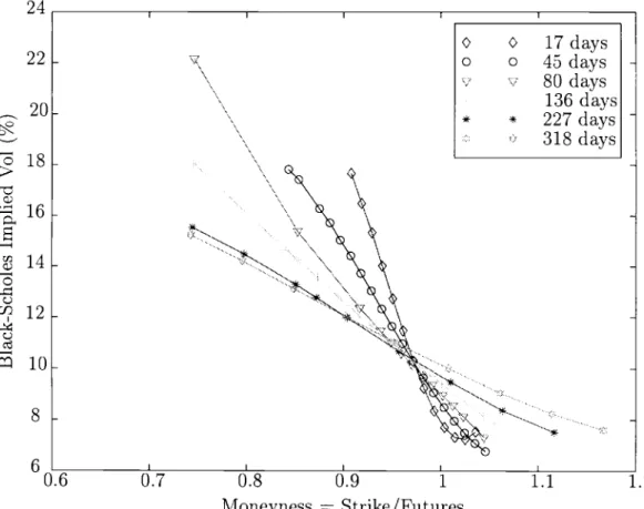
"market-implied" smiles on November 2, 1993, plotted in Figure 1.18 For

each model, calibration was done by minimizing (by choice of the unrestricted parameters) the mean-squared pricing error (MSE), defined as the simple av-erage of the squared differences between the observed and the modeled option

prices across all strikes and maturities. The risk-free rate r is assumed to be 3.19%, and the dividend yield ( is assumed to be zero.

'8The options data are downloaded from the home page of Yacine Ait-Sahalia. There is a total of 87 options with maturities (times to exercise date) ranging from 17 days to 318 days, and strikes prices ranging from 0.74 to 1.17 times the underlying futures price.

-c

I

24

Figure 1: "Smile curves" implied by S&P 500 Index options of 6 different maturities. Option prices are obtained from market data of November 2, 1993.

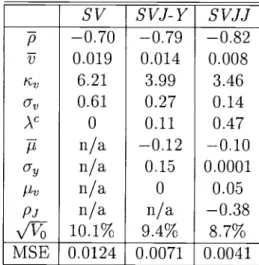
Table 1 displays the calibrated parameters of the models. Interestingly, for this particular day, we see that adding a jump in volatility to the

SVJ-Y model, leading to the model SVJJ model, causes a substantial decline in the level of the parameter a determining the volatility of the diffusion

component of volatility. Thus, the volatility puzzle identified by Bates and

Bakshi, Cao, and Chen, namely that the volatility of volatility in the diffusion

component of V seems too high, is potentially explained by allowing for

jumps in volatility. At the same time, the return jump variance declines

to approximately zero as we replace the SVJ- Y model with the SVJJ model.

A consequence of this is that the jump sizes of Y and of V are nearly perfectly

anti-correlated. This jump distribution reinforces the negative skew typically

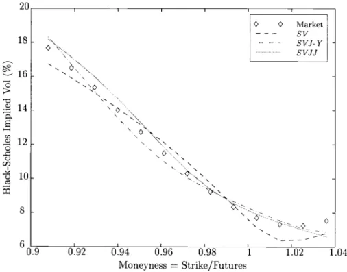
20 I I I I 0 Market

sv

18 _SVJ-Y

16

*

l4

E _'. O'.

12.

N o N -e I N

-0.9 0.92 0.94 0.96 0.98 1 1.02 1.04 Moneyness =Strike/Futures

Figure 2: "Smile curves" implied by S&P 500 Index options with 17 days to maturity. Diamonds are observed Black-Scholes implied volatilities on November 2, 1993. SV is the Stochastic Volatility Model, SVJ- Y is the Stochastic Volatility Model with Jumps in Returns, and SVJJ is the Stochastic Volatility Model with Simultaneous and Correlated Jumps in Returns and \Tolatility. Model parameters were calibrated with options data of

November 2, 1993.

found in estimation of the SVmodel for these data,'9 as jumps down in return

are associated with simultaneous jumps up in volatility.

In order to gain additional insight into the relative fit of the models to the

option data used in our calibration, Figures 2 and 3 show the volatility smiles

for the shortest (17-day) and longest (318-day) maturity options. For both maturities, there is a notable improvement of fit with the inclusion of jumps. Furthermore, the addition of a jump in volatility leads to a more pronounced

smirk at both maturities and one that, based on the relative values of the

'91n addition to the "calibration" results in the literature, see the time-series results of Chernov and Ghysels [1998} and Pan [1998]. For related work, see Poteshman [1998] and

Table 1: Fitted Parameter Values for SV, SVJ-Y, and SVJJ Models

sV

svJ-Y

svJJ

5

—0.70 —0.79 —0.82 17 0.019 0.014 0.008

i

6.21 3.99 3.46

a

0.61 0.27 0.14

)

0 0.11 0.47 71

n/a

—0.12 —0.10

a

n/a

0.15 0.0001 itv

n/a

0 0.05

pj

n/a

n/a

—0.38

\/V

10.1% 9.4% 8.7% MSE 0.0124 0.0071 0.0041

The parameters are estimated by minimizing mean squared

errors (MSE). A total of 87 options, observed on November

2, 1993, are used. /Vj is the estimated value of stochastic volatility on the sample day. The risk-free rate is assumed to be fixed at r= 3.19%, and the dividend yield at (= 0. From "risk neutrality," 71 =_8(1,0) —_1.

MSE in Table 1, produces a better overall fit on this day.

Next, we go beyond this fitting exercise, and study how the introduction of a volatility jump component to the SV and SVJ-Y models might affect the "volatility smile," and how correlation between jumps in Y and V affects the "volatility smirk." We investigate the following three additional special cases:

1. The SVJ-V model: We extend the fitted SVmodel by letting AV = 0.1

and )'

= 0. _{We measure the degree of contribution of the jump}

component of volatility by the fraction i/(a

V0+)

)

ofthe initial

instantaneous variance of the volatility process V that is due to the jump component. By varying the mean of the volatility jumps, three levels of this volatility "jumpiness" fraction are considered: 0, 15%, and 30%. For each case, the time-U instantaneous drift, variance, and correlation are fixed to those implied by the fitted SV model by

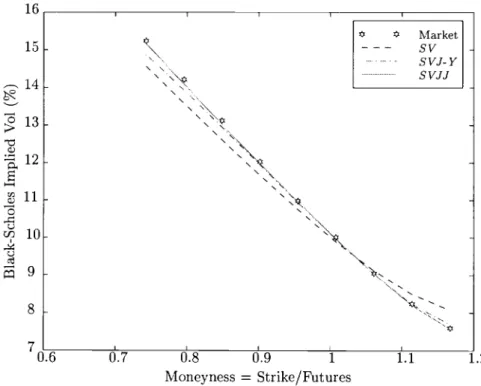
16 I I I I S K' Market 15 Sv • _svJ-Y • S%JJ

14

__________

\

13 12 6

-

11 10 N 0.6 d.7 d.8 d.9 1 1.1 1.2 Moneyness =_{Strike/Futures}

Figure 3: "Smile curves" implied by S&P 500 Index options with 318 days to maturity. Hexagrams are observed implied volatility of November 2, 1993. SV is the Stochastic Volatility Model, SVJ- Y is the Stochastic Volatility Model with Jumps in Returns, and SVJJ is the Stochastic Volatility Model with Simultaneous and Correlated Jumps in Re-turns and Volatility. Model parameters were calibrated with options data of November 2,

1993.

2. The SVJ- Y- V model: We extend the fitted SVJ- Y model by letting

=

ÀY AC = _0, and ÀY be fixed as given in Table 1. Again, the volatility "jumpiness" is measured by the fraction of the instantaneous

variance of V that is due to the jump component. Three jumpiness

levels, 0, 15%, and 30% are again considered. For each case, the in-stantaneous drift, variance, and correlation are matched to the fitted SVJ- Y model.

3. Finally, we modify the fitted SVJJ model by varying the correlation

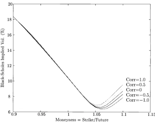
between simultaneous jumps in Y and V. Five levels of correlation are considered: —1.0, —0.5, 0, 0.5, and 1.0. For each case, the means and variances of jumps in V and Y are calibrated to the fitted SVJJ model.

Table 2: "Instantaneous" Moments for the SV and SVJ- V Models

Model

Initial Instantaneous Moments

Drift(V) Var(V) Corr(Y, V)

SV

SVJ-V

tJ—

ic(—Vo)

Vj/iç — V0)

_{a,V0 +Av1L}aV0

+ \v)_1/2

Table 3: Jump Moments for the SVJJ Model

Variables

SVJJ Model: Jump Moments

Mean Variance Correlation

V Y

(VY)

IL?/

Py+PJILv

U+P/i

The implied 30-day "volatility smiles" for the above three variations are plotted in Figures 4, 5, and 6.

4.3 Multi-factor Volatility Specifications

Though our focus in this section has been on jump distributions, we are

also interested in multi-factor models of the diffusion component of stochas-tic volatility. Bates [1997] has emphasized the potential importance of more than one volatility factor for explaining the "term structure" of return

volatil-ities, and included two, independent volatility factors in his model. Similarly,

the empirical analysis in Gallant, Hsu, and Tauchen [1998] of a non-affine, 3-factor model of asset returns, with two of the three state coordinates

ded-icated to volatility behavior, suggests that more than one volatility factor

improves the goodness of fit for S&P500 returns.

Our transform analysis applies directly to any affine formulation of

multi-factor stochastic volatility models, including Bates' model. Here, we also propose an examination of multi-factor volatility models in which there is a

Figure 4: 30-day smile curve, varying volatility jumpiness, and no jumps in returns.

propose consideration of a three-factor model for X (Y 1, V)', given in

its risk-neutral form by

0

cr/1 —

0

(4.6)

where w

is _{an (t)-standard Brownian motion in R3 under Q.}

A _{one-factor volatility model, such as the SV model, may well}

over-simplify the term structure of volatility. In particular, the (SV) model

has an auto-correlation of returns (over successive periods of length z) of

exp(—icz), which decreases exponentially with Li. This _{exponential decay}

is in direct constrast to a common empirical finding of a "long memory"

in volatility. (See, for example, Bollerslev and Mikkelsen [1996] for findings Vol Jumpiness = 0% — - - _{VolJumpiness = 15%} Vol Jumpiness = 30% 17 16 15 14 13 12 11 10 9 8

1

a U rJj U 0.95 1 1.05 Moneyness=Strike/Future 1.1 1.15

(Y\ (r--\

d(V

J

= I ic(V—V)

dt+

\VtJ

\ico(ü—Vj)J

I Up\/V 0 0

ao

18 16 14 12 10 8 Vol

-

- - _Vol Vol Jumpiness = 0% Jumpiness = 15% Jumpiness 30% 1 1.05 Moneyness =Strike/Future

Figure 5: 30-day smile curve, varying volatility jumpiness. Independent arrivals of jumps in returns and volatility, with independent jump sizes.

corr(T4, V+) =

e +

(e°'

— e')

kO/(lc — kO)

(c +ico)a2/ic+

kU/ko

In subsequent work, we plan to further investigate this or related

multi-factor volatility specifications.

6-

0.95 1.1 1.15

based on spot-market data and Pan [1998] for results based on spot-market and options data.) The two-factor volatility model in (4.6), however, yields a more flexible volatility structure. The auto-correlation of z-period returns (with respect to the ergodic distribution of (17, V)) can be calculated for this model to be,

-u

C)

1.15

Figure 6: 30-day smile curve, varying the correlation between the sizes of simultaneous jumps in return and in volatility.

Appendices

A The Affine Jump-Diffusion

This appendix summarizes technical details for the basic AiD model,

allow-ing for time-dependent coefficients.

We fix (,

F,

_{P), a complete probability space, and (F)0<<, a filtration} of sub-a-fields of F satisfying the usual conditions.2° We suppose that there is a strong Markov process X, with (Xi, t) in some D C R x [0, oc) for all

20For technical definitions, see Protter [1990].

t, uniquely solving the stochastic differential equation

pt

XtX0+J

₀

it(Xss)ds+J a(X8,s)dW5+Z,

₀

(Al)

where W is an ()-adapted Standard Brownian motion in _{p: D —+ R,}

a : D —÷

where D is a subset of R

x

[O,) to be defined; Z is a

pure jump process whose jump-counting process N has a stochastic intensity

{.\(X, t) : t > O}, for some )..: D —* [0, oo), and whose jump-size distribution

is Vt, a probability distribution on II depending only on t. It is assumed

that, for each t, {x : (x, t) E D} contains an open subset of R.

We can equally well characterize the behavior of X in terms of the in-finitesimal generator V of its transition semigroup, defined by

Vf(x, t)

ft(x, t) + f(x, t)(x, t) + tr

[f(x,

t)a(x, t)a(x, t)T]

+

(x,t) f

[f(x

+ z,t) - f(x,t)] dvt(z),

_(A.2)

for sufficiently regular f : D —* R. The generator V is defined by the

property that, for any f in its domain, {f(Xt, t) — f Vf(X, s) ds : t >_0} is

a martingale. (See Ethier and Kurtz [1986] for details.) In Appendix F, we consider more general jump behavior.

We impose an "affine" structure on i, aaT, and

\, in that

t(T, t) = K0(t) + K,(t) x (A.3)

a(x,t)a(x, t)T = H0(t)

+ H(t) xk

(A.4)

(x,

t) = 10(t)

+ l,(t) x,

(A.5)

where for each t 0, Ko(t) is n >< 1, K1(t) is n x n, Ho(t) is n x ii and

symmetric, H1 (t) is a tensor2' of dimension n x n x ii, with symmetric

H(c)(t) (for k =

1,. _,

ii), 10(t) is a scalar, and l,(t) is n x 1. The

time-dependent coefficients K = _(K0,

K1), H =

_(H0,

H,), and 1

_{(lo, 1) are} bounded continuous functions on [0, oo). We further assume that, for each

21Let H be an n x n x n tensor, fix its third index to k, the tensor is reduced to an n x n matrix H(') with elements, H =_H(i,j,k).

t > 0, f )(X, s) ds < oo P-as. This type of "affine jump-diffusion"

pro-cess is introduced in Duffie and Ran [1996] for purposes of term-structure

modeling.

We know that a(x, t) must be well defined for all (x, t) in D; indeed one

can define regularity conditions on t, _a, A, and ii such

that a solution X

exists for D = _{{(x,t) a(z, t)a(x, t)T} is _{positive semi-definite}. See Duffie} and Ran [1996] and Dai and Singleton [1999] for additional details. The

conditions would include the requirement that for any (x, t) E D, we have (x + z,t) E D for all zin the support of Vt.

LettingC denote the set of n-tuples of complex numbers, we let O(c, t) =

exp(c. z) di-'t(z), for any c E Ctm such that the integral is well defined.

This "jump transform" 9 determines the probability distribution of each jump measure Vt. Weassume that 9 is measurable.

B Transform Analysis

Fixing T e [0, oc), the objective of this appendix is to compute the transform 02 x D

x

llt

x R+ —+Cof XT conditional on .F, whenever well defined by

(u,X,t,T) E (exp (_JTR(xS,s)ds) exp(u•XT)

(B.1)

where R(x,t) =_po(t)+pi(t) •x, for bounded measurable Po : [0,T] —*Rand

p: [0, T] —+Rtm. The characteristic x = _{(K,H, 1, 9, p) determines i. 1vVith}

technical regularity conditions, we can show that

=

where

x, t, T) =exp

(a(t,

T,u) + 13(t, T, u) x), (B.2)

where i and a satisfy the complex-valued ordinary differential equations

(t,T,u) +B((t,T,u),t) =

0,

(T,T,u) =

u, (B.3)

T, u) + A((t, T, u), t) =0, a(T, T, u) =0, (B.4)

and where, for any c E 02,

8(c, t) =K1(t)Tc + cTH1(t)c — pi(t)

+

11(t) (9(c, t) — 1) (B.5)

A(c, t) = K0(t) c_{+ cTHo(t)c — po(t) + 10(t)(O(c,t)} —

and where (cTH1(t)c) denotes the n-vector with k-th element CTH(k)(t)c

Our results will exploit the following technical conditions.

Definition 1:

_{A characteristic (K, H, 1, 0, p) is well-behaved at (u, T) E}

C' x [0, cc) if there is a unique solution X to (A.1) for 0 <t <T and for an

initial condition (X0, 0) _{D; if (B.3)-(B.4) are solved uniquely by 3 and c;}

and if

(i) E (i dt) <cc, where it t (9((t, T, u), t) —

1)

t),

1/2

(ii) E [(10Tflt

dt) ]

<cc,

where m = Wt

(t, T, u)Ta(Xt

_t), and

(iii) E('I'TD<cc,

where, for each t <T,

=

_exp

(—

f R(X,

s) ds) exp (a(t, T, u) + (t, T, u) Xe).

(B.7)

Proposition 1 (Transform of X): Suppose (K, H, 1,9, p) is well-behaved

at (u, T). Then W is a martingale, and the transform of X defined by (B.1) exists and is given by (B.2).

Proof: By Ito's formula,22

Pt

Wo + J W8tw(s) ds

+ J

i

dW5 + J,

(B.8)

0 0

where

(t) =

a(t,

T, n) + A((t, T, n), t) + [i3(t T, n) + 8(13(t, T, n), t)]

and

=

() —

— f ds,

0<T(i)<t 0

where r(i) = inf{t : N,, = i} is the i-th jump time. Under condition (i),

Lemma 1, to follow, shows that J is a martingale. Under condition (ii), fridW is a martingale. Using (B.3) and (B.4), 0, and we are done.

I

Lemma 1: Under the assumptions of Proposition 1, J is a martingale.

Proof: Letting E,, denote F-conditional expectation under P, for 0

t <

s <T, we have

E,, (

(W() — =

E,, (

E

(w(i)

—

XT(i)_Y(i)))

t<T(i)<S t<T(i)<S = _E,,

(

Wr(i)_ (O(b((i)), (i)) — 1)

\t<T(i)<s r(i)

= E (

f

W

(O(b(u), u) — 1)

dN

Jr(i—1)+ E,, _{(fT W (O(b(u), n) — 1)}

dNa)

Because {W,, (O(b(t), t) — 1):t > 0} is an (Ft)-predictable process, and the jump-counting process N has intensity {.\(X,,, t) : t < T}, integrability con-dition (i) implies that23

E (fS

W_(O(b(u), u) —1)

dATa) E,, (f8 W (O(b(u), n) —1)A(X, u) du)

Hence J is a martingale.

I

C

Transform Inversion

Proposition 2 (Transform Inversion):

Suppose, for fixed T E [O,), a eR, and bE R71, that = (K, H, 1, 0, p) is well-behaved at (a+ivb,T), for

23See, for example, page 27 of Brémaud [1981]. We are applying the result for the real and imaginary components of the integrand, separately.

any v E R, and that

fx(a+ivb,x,o,T)dv < oc,

(C.1)

where '/ is defined by (B.2). Then Ga,b(

;x,T,x)

is well defined by (2.8) and given by (2.9).

Proof: For 0 < < oc, and a fixed y E R,

[ e'/(a

— _{ivb,x, 0, T) —}

ei/'X(a

_{+ ivb, x, 0, T)}

dv

2ir J_

iv 1 rT 1

e_iv) —

e(z_y) I

I

. dGa,b(z;x,T,x)dv iv 1

r r

e_(z_Y)— —

I I

_{. dvdGa,b(z; x, T, ),} iv

where Fubini is applicable24 because

urn Ga,b(y; x, T, x)

x(a,

a, 0, T) <cx, given that xis _{well-behaved at (a, T).}

Next we note that, for > 0,

fT e_(z_Y) e(z_y) dv = sgn(z — y) fT sin(vz

—

dv

J— iv

J v

is bounded simultaneously in z and

,

for each fixed y.25 By the bounded

convergence theorem,

1 f

e"YX(a —_{ivb,x, 0, T) —}

e/(a

_{+ ivb, x, 0, T)}

lim—

i dv T—

2ir J_

iv = —

f sgn(z

—y)dGa,b(z;x,T,x) —

x(a,x,0,T)

+ (Ga,b(y;x,T,x) +Ga,b(y;T,T,x)),

24Here, we also use the fact that, for any n,v E R, e' —_{e"I <} — uI.

where Ga,b(y;x,T, x) =

1imz+,<

Ga,b(z;x,T, x). Using the integrability

condition (Cl), by the dominated convergence theorem we have r, 0, T)

Ga,b(y;x,T,x) =

2

+

J_ f

e''(a

— ivb,x, 0, T) —

e/(a

+ ivb, x, 0, T) dv

47rJ_

iv

Because /'X(a —_{ivb,x, 0, T) is the complex conjugate of /x(a + ivb, x, 0, T),} we have (2.9).

I

We summarize our main option-pricing tool as follows.

Proposition 3. The option-pricing formula (2.7) applies, where G is

com-puted by (2.9), provided:

(a) x

is well-behaved at (d — _ivd,T) and at (—ivd, T), for all v E l, and

(b) fRX(d_ivd,x,0,T)dv <

, and

fR/,X(_ivd,x,0,T)dv <oc.

D Change of Measure

This appendix provides the impact of a change of measure defined by a

density process or a state-price-density process that is of the exponential-affine form in an exponential-affine jump-diffusion state process X.

Fixing T >0, suppose, under the measure P, that a given characteristic

x

(K,H, 1, 0, p) is well-behaved at (b, T) for some b e R''. Let

et=ex(_f

(D.1)

Under the conditions of Proposition 1, is a positive martingale. We may then define an equivalent probability measure Q _by

=

_CT/o.

In this section, we show how to compute the transform of Xaftera change

of measure that arises from a normalization associated with .

Proposition

4 (Transform under Change of Measure):

Let (Q)

= (KQ,H, i, OQ) be defined by

K(t) =

K0(t)+ H0(t)/3(t, T, b) ,

K(t)

=

K1(t)+ H1(t)3(t, T, b), (D.2)

1(t) =

10(t)0(13(t, T, b), t) ,

l(t)

=

11(t)0(13(t,T, b), t), (D.3)

where H1(t)b(t) denotes the n x n matrix with k-th column H(t)b(t). Let

R(a, t) —

p(t)

+ p(t) x, for some bounded measurable p : [0, cx) —+ JR

and p : [0, oc) R. Let Q =

be such that x(Q) iswell-behaved

at some (u,T). Then, fort < T,

E (exp (_f

RQ(X8,s)ds)

exp(UXT)

x(Q)(u,x,t,T),

(D.5)

where ') is defined by (B.2).

Proof:

Let

=

W

— f

a(X,

8)T(8

_{T,b) ds,} t > 0. _(D.6)

Lemma 2, below, shows that is a P-local martingale. It follows that

w

is_{a Q-local martingale. Because 10t a(X8,s)/3(s, T,}b) ds is a continuous

finite-variation process, {W, W39] =

[W',

T4f]t

= 6(i,j)

t, where (.)

is the

kronecker delta. By Levy's Theorem, wis a standard Brownian motion in R' under Q.

Next,we let

M =

N

— f

O((s,T, b))(X8, s) ds, t > U. (D.7)

Lemma 3, below, shows that eM is a P-local martingale. It follows that M is a Q-local martingale. By the martingale characterization of

inten-sity,26 we conclude that, under Q, Nis a counting process with the intensity

{A(X,t) : t o} defined by )(x,t)

l(t) + 1(t) x.

Using the fact that, under Q,

T4'

is a standard Brownian and the jump

counting process N has intensity {AQ(X, t) : t > o}, we may mimic the

proof of Proposition 1, and obtain (D.5) replacing in the proof of Lemma 1

E (t<r(i)<T

(W() — with

E (

(W() —

=

(

_{eT(i) (W()}—

I

This completes the proof.

I

Lemma 2: Under the assumptions of Proposition 1, WQ is a P-local

martingale.

Proof: By Ito's Formula, with 0 <s < t < T, — SW +

f dW + f

W

d

+

—

)

(w

— w) +

ft

d[,

W]

s<'u<t S +

ft

(dW

—_{aT(Xu, u)b(u)} du)

+

ft W

d +

ft aT(X u)b(u)

du

e5w+f

dW+f

Wde,

where [, WQ]c denotes the continuous part of the "square-brackets"

pro-cess [, WQ]. As W and are P-martingales, both {f dW : t> o} and

{

f

W : t o} are P-local martingales. Hence,

is a P-local mar-tingale. I

Lemma 3:

Under the assumptions of Proposition 1, M' is a P-local

martingale.

Proof: By

Ito'sFormula, with 0 < s

<t T,

SM +f

_dM

+fMd +

(

— N_)

S S

s<u<t

=

+

ft dM + ft

M d + je,

where

M =

N

—

f

_{(X5, s) ds, and where}

J =

(

—

— ftu(9((uTb),u)

—

1)(X,u)du.

AsMandareP-martingales, {f0_dM : t> o}

and

{fM_d : t

o} are P-local martingales. By a proof similar to that of Lemma 1, and using the Integration Theorem (y) in Brémaud [1981], we can show that J is a P-local martingale. I

Forthe remainder of this appendix, we denote Q by _{Q(b), emphasizing}

the role of bin defining the change of probability measure given by (Dl). We

let (b) = (KQ(b),

HQ(b), 1Q(b),9Q(b), p) denote the associated characteristic.

The previous result shows in effect that, under Q(b), the state vector X is

still an affine jump-diffusion whose characteristics can be computed in terms

of the characteristics of X under the measure P. This result provides us with an alternative approach to option pricing. We suppose that Q(O) is

an equivalent martingale measure. The price F (X0, a, d, c, T) of an option paying (ea+dXT —c) + at T is given by

F (X0, a, d, c, T) = E° (exp (

1T

R(XS, s) ds) (eT —

=

eaEo)

(exp

(_

f R(XS, s)

ds) eT1d.xT>fl(c)_a)

—

eE°

(exp (_

f R(X8,

s) ds) ld.XTln(c)_a).

Provided the characteristic (K, H, 1, 9, p) is well-behaved at (d, T) and (0, T),

we may introduce the equivalent probability measure Q(d), and write

F (X0, a, d, c, T) = ea exp (c(0, T, d) + 3(0, T, d) . X0) (ld.XT>lfl(c)_a)

—_c

exp ((0, T, 0) + (0, T, 0) .X0) E° (ld.XT>lfl(c)-a).

Let x(')

(KQ(d), 1Q(d) 0Q(d), 0) and x(°) = _(KQ(°), Q(O), 0)

be defined by (D.2)-(D.4) for b = d and b = 0. We suppose that x(')and

x(°)

are well behaved at (ivd, T) for any v eR. Then

Q(d) 1 — 1

1 f

Tm

[j5X(')(ivd, x, 0, T)e()_0)]

E

_{dXT>ln(c)—a)} — — +— _dv, — 2 _71f0 V Q(fJ) (1 — 1

1 f

Tm [x(°)(ivd, x, 0, T)e_iv(n1(c)_a)]

E

_{-'-dXT>1n(c)—a)} — — +— _dv, — 2

Jo

V

provided j

X(1)(ivd,X0, 0, T) dv < oc and j

(°)(ivd,

X0, 0, T) dv < oc. These quantities may now be substituted into the previous relation in order to obtain the option price.

E "Extended" Transform Analysis

In this appendix, fixing a characteristic x, we introduce an extended"

trans-form

: R x C' x D x

x R —+ C of XT conditional on , whenwell

defined for t <T by

u, X, t, T) E (exp (_ f

R(X8,s) ds) (v XT) euXT (E.1) Under additional technical conditions, we can show that

u, x, t, T) =

(u,

x, t, T) (A(t, T, v, u) + B(t, T, v,

x),

(E.2)

where '/" is given by (B.2), and where B and A satisfy the linear ordinary

differential equations

T, v, u) + K1(t)TB(t, T, v, u) + (t, T, n)TH1(t)B(t, T, v, u)

+11(t)e(/3(t,T,u),t) .B(t,T,v,u) =

0,

B(T,T,v,u)

v, (E.3)

T, v, u) + K0(t) B(t, T, v, u) + (t, T, u)TH0(t)B(t, T, v, u)

+ 10(t)e(/3 (t, T, 'u), t) B(t, T, v, =0, A(T, T, v, u) 0, (E.4)

where e(c,t)

=

f.

exp(c. z) z dv(z).

Letting W be defined by (B.7) and t =

'I'

(A(t, T, v, u) + B(t, T, v, u) Xe),

sufficient technical conditions are

fT \

(z) E f0 yt dt) < oc, where

=

\(X,

_{t) ( (O((t, T, u), t) — 1) + WB(t, T, v, e(/3(t,T,}

), t)).

1/2

IT-

-(ii)

E f0 Tit

7it dt) < cc, where

=

((t,T,u)T+B(t,T,v,u)T)a(Xt,t).

(iii) E(T)<cx.

Definition El:

(K, H, 1,0, p) is "extended" well-behaved at (v, u, T), if there is a unique solution X to (A.1) for 0 < t < T, if (B.3)-(B.4) are solved

uniquely by and ,

if

(E.3)-(E.4) are solved uniquely by B and A, and if the above conditions (i)-(iii) are satisfied.

Proposition 5 ("Extended" Transform of X):

Suppose

x

= (K,H, 1, 0, p)

is extended well-behaved at (v, u, T). Then 1 is a martingale, and the

trans-form of X defined by (El) is thus given by (E.2).

In principle, the extended transform can be computed by differentiation of

the transform ,

_justas moments can be computed from a moment generating

function. In practice, this may involve solving the same ODEs (E.3)-(E.4).

For fixed a E W, b E R, and d e

we next define G,o,d( X0, T, x)

by

/

/

fT

Ca,b,d(y; Xo, T, x) = E

J R(X5,

s) ds) (a .XT)

eT1b.xTy

0

(E.5)

Provided x (K,H, 1,0, p) is extended well behaved at (a, d+ ivb, T), for

any v E R, and that f

d + ivb, x, 0, T) dv < , can be obtained

by the Fourier-inversion of so that

Ga,b,d(y;x,

T, ) =

q5(a,d,x, 0, T) —

1 _{Tm [(a, d + ivb, x, 0, T) exp(—ivy)]}

dv.

(E.6)

Now, anticipating the calculation of option prices, we consider, for given

cE Rand b E RTh. T (X0, b, c, T) = EX

(exp (_

f R(X,

s) ds) (b. XT —

c)+).

(E.7) We immediately obtain

/

/ T

C (Xe, b, c, T) = EX (\exp (—

J R(X5,

0 s) ds) (b XT —c)lb.Xy> = Cb,b,o _{(—c; X0, T, x)} — c_{G0,_ (—c; X0, T, x) (E.8)}

where Ga,bis given by (2.9) and Ca,b,O is given by (E.6).

With this calculation, we could price a slope-of-the-yield-curve option, as

yields in an AJD setting are themselves affine. Under the assumption of a deterministic short rate and dividend-yield process, that is, Pi =q1 0, we

may also use this approach to price an asian option. For the latter, struck at

c, at the expiration date T, the option pays (+ dt --_c), where

is the price process of the underlying asset. If Q is an equivalent martingale measure, we must have

dX =

(R(X,

t) — _((Xe,

t)) X dt +

where M is a Q-martingale. For any 0 < t < T, let Y =

j

X ds. For

short rate Po, we can let E5 = (P0,

0) and ,Ei =

(0,0)

0, and see that

X =

_(X,Y) is an (n+ 1)-dimensional affine jump diffusion with characteristic

=

(k,

i, T, ,

) that

can be easily derived from using the fact that d =

x(z)dt. We may then use (E.8) and obtain the initial market value of the

option as

(o,€(m+1,Tc,T).

F Extension to Multiple Jumps

We may easily relax the jump behavior of X to accomodate m types of jumps, with jump type i having jump-conditional distributn v at time t, again depending only on t, and stochastic intensity {.A(X,t) : t 0}, for

i E {1,.., ,

m}, where A : D —*

R

is defined by )j(X,t)

1(t) + l(t) .

for bounded measurable 1 _{((1, if), .} . . , (lv',

if). The jump transforms

o

(0',... ,

0)

_{are defined by 0(c, t) = exp(c. z) di4(z), c e C'.}

We can also characterize the behavior of X with multiple jumps in terms of the infinitesimal generator V of its transition semigroup, with

Vf(x, t) =

ft(x,

t) + f(x, t)(x, t)

+ tr

[f(x, t)u(, t)a(x, t)T]

[f(x+z,t)-f(x,t)] dv(z),

(Fl)

for sufficiently regular f D —+ R.

In this general setting, Propositions 1, 2, and 3 apply after replacing the m

last terms in the right-hand sides of (B.5) and (B.6) with _{11(t) (0 (c, t) —1)}

m

and j1

10(t) (0 (c, t) — 1), respectively.

This can be extended to the case of an infinite number of jump types by allowing for a general Levy jump measure that is affine in the state vector.

(See Theorem 42, page 32, of Protter [1990].)

G Cap Pricing

A cap is a loan with face value, say 1, at a variable interest rate that is capped

at some level .

At

time t, let r, 2, .

. ., nr be the fixed dates for future

interest payments. At each fixed date kr, the p-capped interest payment, or "caplet," is given by (1((k —

1),

_{k) —}

, where

7((k — l)T,kT) is the i-year floating interest rate at time (k —_1)r, defined by

1+r((k—1)r,kr))

=A((k—1)T,kT).

The market value at time 0 of the caplet paying at date k can be expressed

as

/

rkr

Caplet(k) E exp (

—

/

R(X,

u) du) r (((k —

1),

kT) — \' Jo

I

(k—1)r ₁ +

(1+rf)E [ex (_f