w o r k i n g
p
a
p
e
r
04 05
Money in Search Equilibrium, in
Competitive Equilibrium, and in
Competitive Search Equilibrium
Working papers
of the Federal Reserve Bank of Cleveland are preliminary materials circulated to stimulate discussion and critical comment on research in progress. They may not have been subject to the formal editorial review accorded official Federal Reserve Bank of Cleveland publications. The views stated herein are those of the authors and are not necessarily those of the Federal Reserve Bank of Cleveland or of the Board of Governors of the Federal Reserve System.Working papers are now available electronically through the Cleveland Fed’s site on the World Wide Web:
www.clevelandfed.org/Research.
Guillaume Rocheteau is at the Federal Reserve Bank of Cleveland and may be reached at
Guillaume.Rocheteau@clev.frb.org. Randall Wright is at the University of Pennsylvania and NBER . The authors thank Ricardo Lagos and Matthew Ryan for their input, as well as Ruilin Zhou, David Levine, three anonymous referees, and participants at the Society for Economic Dynamics in Paris, the Canadian Macro Study Group in Toronto, the Federal Reserve Banks of Cleveland, Minneapolis and Philadelphia, the Universities of Chicago, Northwestern, Victoria, Paris II, Penn, Yale, MIT, Michigan, Iowa and Essex for comments. The authors are grateful to the Summer Research Grant scheme of the School of Economics of the Australian National University, the National Science Foundation, the Central Bank Institute at the Federal Reserve Bank of Cleveland, and ERMES at Paris 2 for research support.
Working Paper 04-05
July 2004
Money in Search Equilibrium, in Competitive Equilibrium, and in
Competitive Search Equilibrium
By
Guillaume Rocheteau and Randall WrightWe compare three market structures for monetary economies: bargaining (search equilibrium); price taking (competitive equilibrium); and price posting (competitive search equilibrium). We also extend work on the microfoundations of money by allowing a general matching technology and entry. We study how equilibrium and the effects of policy depend on market structure. Under bargaining, trade and entry are both inefficient, and inflation implies first-order welfare losses. Under price taking, the Friedman rule solves the first inefficiency but not the second, and inflation may actually improve welfare. Under posting, the Friedman rule yields the first best, and inflation implies second-order welfare losses.
JEL Classification: E40, E50
1. INTRODUCTION
We compare three models of monetary exchange that differ in terms of their
assumed market structures. In the first, at least some activity takes place
in highly decentralized markets where anonymous buyers and sellers match randomly and bargain bilaterally over the terms of trade. Following the
literature, we call this search equilibrium. In the second model there are
still frictions, and in particular agents are still anonymous, but they meet
in large markets where prices are taken as given. We call this competitive
equilibrium. In the third model, we assume there are different submarkets with posted prices and buyers and sellers can direct their search across these submarkets, although within each submarket there are again frictions. We
call thiscompetitive search equilibrium. In each case, we provide results on
existence and on uniqueness or multiplicity of equilibrium. We also analyze efficiency and optimal monetary policy.
The underlying framework is related to recent search-theoretic models of money following Lagos and Wright (2002) — hereafter referred to as LW. The key assumption in this framework is that, in addition to the activity that takes place in the more or less decentralized markets described above, agents also have periodic access to centralized competitive markets. The existence of the decentralized markets, and in particular the assumption that agents are anonymous, generates an essential role for money (Kocherlakota (1998), Wallace (2001)). The existence of the centralized markets greatly
simplifies the analysis, because when combined with the assumption that
preferences are quasi-linear, it implies that all agents of a given type will carry the same amount of money into the decentralized market. This renders
the distribution of money holdings in this market simple, which makes the model very easy to analyze, compared to similar models with no centralized markets like Green and Zhou (1998), Molico (1999), Camera and Corbae
(1999), or Zhou (1999).2
Intuitively, the simplification comes from the fact that quasi-linearity
eliminates wealth effects on the demand for money, and hence eliminates dispersion in money holdings based on trading histories. While we believe that the wealth/distribution effects from which we are abstracting are inter-esting, as discussed in Levine (1991) and Molico (1999) e.g., the goal here
is to focus on other effects that have not been analyzed previously.3 To
introduce these new effects we extend existing monetary models by adding a generalized matching technology and a free entry condition. These ex-tensions can be thought of as being adapted from labor market models like those discussed in Pissarides (2000). Their role here is to allow us to discuss
the effects of inflation on the extensive margin (the number of trades) as well
as the intensive margin (the amount exchanged per trade), and to discuss “search externalities” — i.e. the dependence of the amount of trade on the composition of the market.
2Shi (1997) provides a different approach that also delivers simple distributions; see LW
for a comparison. Note also that, as emphasized by Zhou (1999) and Kamiya and Shimizu (2003), a problem with some of the models mentioned above is that they have a continuum of stationary equilibria. This is not true in the LW model, even if we generalize preferences away from quasi-linearity, for the following reason. In the models in Zhou or Kamiya and Shimizu, there are equilibria where agents value money only in integer multiples ofp; i.e. the value of havingmdollars,V(m), is a step function with jumps as atp,2p,3p...Given this, nothing actually pins downp. With periodic competitive markets as in LW, however,
V(m)must be strictly increasing, and such equilibria do not arise.
3
Moreover, although our specification ignores wealth effects, recent work suggests the results are robust in the following sense. Khan, Thomas and Wright (2004) solve numer-ically a version of the model in LW with a more general class of utility functions, and show that as the wealth effects get small, both the distribution of money holdings and the welfare cost of inflation converge to the results derived analytically for quasi-linear specification.
Our main result is to show that the different market structures have very different implications for the nature of equilibrium and for the effects of policy. In search equilibrium (bargaining), we prove that the quantity
traded and entry are both inefficient. In this model inflation implies afi
rst-order welfare loss, and although the Friedman Rule is the optimal policy, it cannot correct the inefficiencies on the intensive and extensive margins. In competitive equilibrium (price taking), the Friedman Rule gives efficiency along the intensive margin but not the extensive margin. In this model the
effects of policy are ambiguous, and inflation in excess of the Friedman Rule
may be desirable. In competitive search equilibrium (posting), the Friedman
Rule achieves thefirst best. In this model inflation reduces welfare but the
effect is second order. We think these results are interesting because they help to sort out which results in recent monetary theory are due to features of the environment — preferences, information etc. — and which are due to the assumed market structure — bargaining, posting etc.
The three market structures have previously been used, of course, in different contexts. In the context of monetary economics, dating back to Shi (1995) and Trejos and Wright (1995) most search-based models use bargaining. Competitive pricing is used in, say, overlapping generations models by Wallace (1980) and turnpike models by Townsend (1980), but it has not been used in monetary models with search-type frictions. Price posting and directed search have been used in several monetary models (see Section 5 for references), but not in combination, and it is the combination that is critical for the concept of competitive search equilibrium. In terms of the literature on labor markets, one way to understand the three market structures is the following. Our bargaining model is monetary economics’
analog to the Mortensen and Pissarides (1994) search model; our price-taking model is the analog to the Lucas and Prescott (1974) search model; and our price-posting model with directed search is the analog to Moen (1997) and Shimer (1996).
From a different perspective, consider Diamond (1984), who introduced a cash-in-advance constraint in the Diamond (1982) model because he wanted to discuss “Money in Search Equilibrium.” Although his approach to bar-gaining was primitive at best, perhaps a bigger problem was that money is imposed exogenously via the cash-in-advance constraint. Later, Kiyotaki and Wright (1991) showed that in a very similar environment a role for
money can be derived endogenously. Kocherlakota (1998) clarified exactly
what makes money essential in those environments: a double coincidence problem, imperfect enforcement, and anonymity. It seems natural to look for a physical environment that incorporates these features, but also allows one to consider alternative market structures. Here, in addition to being able to discuss what Diamond wanted we can also analyze “Money in Com-petitive Equilibrium” and “Money in ComCom-petitive Search Equilibrium.”
The rest of the paper is organized as follows. Section 2 presents the basic assumptions and discusses efficiency. Section 3-5 analyze equilibrium in the models with bargaining, price taking, and price posting. Section 6 concludes by summarizing the results.
2. THE BASIC MODEL
Time is discrete and continues forever. As in LW, each period is divided into two subperiods, called day and night, where economic activity will dif-fer. During the day there will be a frictionless centralized market, while at
night there will be explicit frictions and trade will be more or less decentral-ized, depending on which model (market structure) we consider. There is a continuum of agents divided into two types that differ in terms of when they
produce and consume. Wefind it convenient to call thembuyers andsellers.
The sets of buyers and sellers are denotedB andS, respectively. The
differ-ence is the following: while all agents produce and consume during the day, at night buyers want to consume but cannot produce while sellers are able to produce but do not want to consume. This generates a temporal double coincidence problem at night. Combined with the assumption that agents are anonymous, which precludes credit in the decentralized night market,
this generates an essential role for money.4
It is well know by now that several different models can generate a similar
role for money, including a variety of specifications with many goods and
specialization in tastes and technologies (e.g. Kiyotaki and Wright (1989, 1993)). We choose to work with a single consumption good and a temporal double coincidence problem for the following reason. In the typical search-based model, any agent engaged in decentralized trade may end up either buying or selling, depending on who they meet, while here sellers can only sell and buyers can only buy in the night market. Differentiating types ex ante allows us to introduce an entry decision on one side of the decentralized market, and thereby allows us to capture extensive margin effects in a very
simple way. Thus, the measure of B is normalized to 1 and all buyers
participate in the night market at no cost, while only a subsetSt⊆S with
measure nt of sellers enter the night market at each date t, and we will
4
Essential in this context means we can achieve allocations with money that we could not achieve without it; again see Kocherlakota (1998) and Wallace (2001).
consider both the case wherent is exogenous and where sellers may or may
not choose to enter at costk.5
Money in the model is perfectly divisible, and agents can hold any non-negative amount. The quantity of money per buyer grows at constant rate
γ: Mt+1 = γMt. New money is injected, or withdrawn if γ < 1, by
lump-sum transfers in the centralized market. For simplicity we aslump-sume these transfers go only to buyers, but this is not essential for the results (i.e., things are basically the same if we also give transfers to sellers, as long as they are lump sum in the sense that they do not depend on behavior, and in particular, on their entry decisions). Also, we restrict attention to policies
whereγ≥β, where β is a discount rate to be discussed below, since it can
easily be checked that forγ < βthere is no equilibrium. Furthermore, when
γ=β — which is the Friedman Rule — we only consider equilibria obtained
by taking the limit γ → β. In general, at date t the distribution of (real)
money holdings across buyers isFtb and the distribution across sellers isFts.
The instantaneous utility of a buyer at datet is
Utb =v(xt)−yt+βdu(qt), (1)
wherextis the quantity consumed and ytthe quantity produced during the
day,qtis consumption at night, andβdis a discount factor between day and
the night. There is also a discount factor between night and the next day,
5When we allow entry, we assume the set
Sis large enough thatntis never constrained.
Also, as in standard search models with constant returns, we are only interested in the ratio of buyers and sellers and not the overall size of the market; this is why we have entry by one side only. There are alternatives to entry that can be used to endogenize the extensive margin. For example, Rocheteau and Wright (2004) consider afixed total number of agents that can choose whether to be buyers or sellers. In a related model Lagos and Rocheteau (2003) keep the buyer-seller ratio fixed but introduce endogenous search intensity.
βn, and we let β = βdβn < 1.6 Lifetime utility for a buyer is P∞t=0βtUtb. We assume u(0) = 0, u0(0) =∞,u0(q)>0, andu00(q)<0. Also, v0(x)>0, v00(x)<0 for all x, and there exists x∗ >0 such that v0(x∗) = 1. Without loss of generality, we normalizev(x∗)−x∗= 0. Similarly, the instantaneous utility of a seller is
Uts=v(xt)−yt−βdc(qt), (2)
where xt is consumption and yt production during the day, and qt is
pro-duction at night. Lifetime utility for a seller is P∞t=0βtUts. We assume
c(0) = c0(0) = 0, c0(q) > 0 and c00(q) > 0. Also we assume c(q) =u(q) for someq >0, and letq∗ denote the solution to u0(q∗) =c0(q∗).
In the centralized day market the price of goods is normalized to1at each
datet, while the relative price of money is denotedφt. In the decentralized night market, details in terms of prices will differ across the models studied below, but there will always be some friction in the following sense: each
period t only a subset Bet ⊆ B of buyers and a subset Set ⊆ St ⊆ S of
sellers who participate get to trade in this market. Agents in Bet∪Set may
either trade bilaterally or multilaterally in the models discussed below. The measure of Bet is αb(nt) and the measure of Set is ntαs(nt), and we assume
agents in these sets are chosen at random; hence the probabilities of trading for buyers and sellers at night are αb(nt) and αs(nt), respectively. This
allows for “search externalities” in the sense that trading probabilities may
depend on the ratio of sellers to buyers, nt. Typically, unless otherwise
indicated we assume αb(n) = α(n) and αs(n) = α(n)/n, which means the
6A special case is when agents do not discount between one subperiod and the next,
i.e. eitherβn= 1orβd= 1, as in LW. Another special case is whenβd=βn, so that the
two subperiods can be thought of as even and odd dates, as in the version of the model studied by Williamson (2004).
same number of buyers and sellers trade in the decentralized market, but
we also discuss some cases where we relax this. We also assumeα0(n)>0,
α00(n)<0,α(n)≤min{1, n},α(0) = 0,α0(0) = 1 and α(∞) = 1.7
We now consider efficiency, which of course can be discussed indepen-dently of the assumed market structure and prices. Consider a social planner
who chooses each period the measure nt of sellers in the night market, as
well as an allocation At = [qtb(i), qst(i), xt(i), yt(i)] specifying consumption
and production during the day [xt(i), yt(i)] for all i∈ B∪S, consumption
at nightqtb(i)for alli∈Bet, and production at nightqst(i)for alli∈Set. The
planner is constrained by the frictions in the environment, in the sense that
he cannot actually choose Bet and Set, but only nt, and then these sets are
determined at random in such a way thatBethas measureαb(nt)and Sethas
measurentαs(nt). In the case where the same number of buyers and sellers
trade in the decentralized market,Bet and Setboth have measure α(nt).
Given quasi-linear utility, we only consider the case where the planner weights all agents equally. Thus, let
Wt = Z B∪S{ v[xt(i)]−yt(i)}di +βd Z h Bt u[qtb(i)]di−βd Z h St c[qst(i)]di−βdknt. (3)
The planner wants to maximize P∞t=0βtWt. Feasibility requires several
things. First, we obviously must haveRB∪Sxt(i)di≤ R B∪Syt(i)di. Similarly we must have RBh tq b t(i)di ≤ R h Stq s
t(i)di, but in addition, in a model where
7
The functionα(n)can be given several interpretations; for now one can think of it as the standard specification coming from a constant returns to scale matching technology. Thus, if µ(nb, ns) is the number of meetings when there are nb buyers and ns sellers,
constant returns implies the arrival rate for a representative buyer isαb=µ(nb, ns)/nb= α(ns/nb). See Petrongolo and Pissarides (2001) for an extensive discussion of the matching
agents trade bilaterally at night, we have the stronger requirementqtb(i) ≤
qts(j) for each trading pair (i, j). An efficient outcome is defined as paths
forntand At that maximize P∞t=0βtWt subject to these restrictions.
PROPOSITION 1: An efficient outcome is stationary and satisfies: x(i) =
x∗ for all agents in the day market; qb(i) = qb and qs(i) =qs for all i∈Be and allj∈Se,whereu0(qb) =c0(qs)and α
b(n)qb =nαs(n)qs; and
α0b(n)hu(qb)−qbc0(qs)i+ [αs(n) +nα0s(n)][qsc0(qs)−c(qs)] =k. (4)
In the case where αb(n) = nαs(n) = α(n), this implies qb(i) = qs(j) = q∗
and n=n∗, where
α0(n∗) [u(q∗)−c(q∗)] =k. (5)
PROOF: Notefirst that the planner’s problem is equivalent to a sequence
of static problems. Maximizing Wt at each date leads to first order
condi-tions that imply v0[x(i)] = 1, and therefore x(i) = x∗ for all i in the day
market, andu0[qb(i)] =c0[qs(j)] =λ/βdfor alliandjthat trade in the night
market whereλis the Lagrange multiplier associated with the feasibility
con-straintRBhqb(i)di=RShqs(i)di. From the feasibility constraint, sinceBeandSe have measuresαb(n) andnαs(n), respectively, we haveαb(n)qb =nαs(n)qs.
Given this, thefirst order condition fornis (4). Finally, (5) is derived from
(4) by using qs =qb and αs(n) +nα0s(n) =α0(n). Q.E.D.
As long as x =x∗, which will turn out to be true in every equilibrium
considered below, and ignoring constants, for anynandqwelfare per period
can be measured by α(n) [u(q)−c(q)]−kn. From this it is clear that the efficientqis the one that solvesu0(q∗) =c0(q∗), and as seen in (5) the efficient
nis the one that makes a seller’s marginal contribution to the trading process
3. SEARCH EQUILIBRIUM (BARGAINING)
In this section we study the market structure used in much of the recent literature on the microfoundations of money, where buyers and sellers trade bilaterally and bargain over the terms of trade. In this model, one can think
of the event that a buyer gets to trade as the event that he meets a seller,
and vice-versa, as in standard matching models. In the following we define
the real value of an amount of money mt in the hands of an agent at date
t by zt =φtmt. Here we focus on steady-state equilibria, where aggregate
real variables, including the aggregate real money supply Zt = φtMt, are
constant. Therefore, in steady-state equilibrium, we have φt+1/φt = 1/γ
becauseMt+1/Mt=γ.
If a buyer with real balances zb meets a seller with zs, let d=d(zb, zs)
and q = q(zb, zs) denote the real dollars and units of the good that are
traded. LetVb(z
b) andWb(zb)be the value functions for a buyer withzb in
the night market and day market, respectively, and letVs(zs) and Ws(zs)
be the value functions for sellers. Bellman’s equation for a buyer in the decentralized night market is
Vb(zb) = α(n) Z ½ u[q(zb, zs)] +βnWb · zb−d(zb, zs) γ ¸¾ dFs(zs) + [1−α(n)]βnWb µ zb γ ¶ . (6)
In words, with probabilityα(n) he meets a seller who has a random zs, at
which point he consumesq(zb, zs)and starts the next day with real balances
the next day withzb/γ.8 Similarly, for sellers, Vs(zs) = α(n) n Z ½ −c[q(zb, zs)] +βnWs · zs+d(zb, zs) γ ¸¾ dFb(zb) + · 1−α(n) n ¸ βnWs µ zs γ ¶ −k. (7)
Comparing (6) and (7), notice only sellers pay the participation costk.
In the centralized day market a buyer’s problem is Wb(zb) = max ˆ z,x,y n v(x)−y+βdVb(ˆz) o (8) subject tozˆ+x=zb+T +y, (9)
where T is his real transfer and zˆ is the real balances he takes into that
period’s decentralized market.9 Similarly, for any seller who enters the night
market, Ws(zs) = max ˆ z,x,y{v(x)−y+βdV s(ˆz) } (10) subject tozˆ+x=zs+y. (11)
LEMMA 1: For all agents in the centralized market,zˆis independent of
z. Also,Wb(zb) =zb+Wb(0) andWs(zs) =zs+Ws(0)are linear.
PROOF: Consider a buyer. Substituting (9) into (8), we have Wb(zb) =zb+T+ max
ˆ z,x
n
v(x)−x−zˆ+βdVb(ˆz)o. (12)
The rest is obvious. Q.E.D.
8
If a buyer holdszt=mtφt at the end of periodt, his real balances at the beginning
of periodt+ 1arezt+1=mtφt+1=ztφt+1/φt=zt/γ.
9
We are ignoring non-negativity constraints. For variables other thany, these will be satisfied under the usual conditions. Fory, we simply look for equilibria with the property thaty >0for all agents, but one can impose conditions on primitives to guarantee this is valid, as in LW. It is important thaty≥0is not binding for a key result proved below — the result that all agents of a given type choose the sameˆz, independent ofz.
Assuming Vb is differentiable (it will be) the first order condition for zˆ
from (12) is
−1 +βdVzb(ˆz)≤0, = 0ifz >ˆ 0, (13)
and ifVb is strictly concave over the relevant range (it will be under weak
conditions) there is a unique solution to (13) and all buyers choose the same
ˆ
z.10 Similarly all sellers choose the sameˆz. To say more, we need to discuss
the terms of trade in the decentralized market.
Consider a meeting between a buyer withzb and a seller withzsat night.
To determineq(zb, zs)andd(zb, zs)in this model we use the generalized Nash
bargaining solution, whereθ∈(0,1]is the bargaining power of a buyer and
threat points are given by continuation values. Thus, the payoffs of the buyer and seller areu(q) +βnWb[(zb−d)/γ]and −c(q) +βnWs[(zs+d)/γ], and
the threat points areβnWb(zb/γ)andβnWs(zs/γ). Linearity ofWb(zb)and
Ws(zs) implies Wb[(zb−d)/γ]−Wb[zb/γ] = −d/γ and Ws[(zs+d)/γ]−
Ws[zs/γ] = d/γ. Hence the generalized Nash bargaining solution reduces
to max q,d · u(q)−βn γ d ¸θ· −c(q) +βn γ d ¸1−θ (14)
wheredis subject to the resource constraintd≤zb.
It is immediate that the solution to (14) is independent ofzs. Moreover,
(q, d)depends on zb if and only if the constraintd≤zb binds. If it does not
bind, thefirst order conditions from (14) are
u0(q) = c0(q), (15)
βn
γ d = (1−θ)u(q) +θc(q) (16)
1 0LW provide details on the existence, differentiability, and strict concavity of the value
functions for their version of the model, and the same arguments apply here. We will discuss how things change in the other models considered below.
which imply q = q∗ and d = z∗ = [θc(q∗) + (1−θ)u(q∗)]γ/βn. If the
constraint does bind, then q solves thefirst order condition from (14) with
d=zb, which we can write as
βn
γ zb =g(q, θ) =
θu0(q)c(q) + (1−θ)c0(q)u(q)
θu0(q) + (1−θ)c0(q) . (17)
For future reference, note that the function g(q, θ) defined in (17) satisfies gq(q, θ)>0 for all q < q∗.
This fully describes decentralized trade under bargaining. To return to
the determination ofz, we now make the following assumption:ˆ
ASSUMPTION 1: (i) limq→0u0(q)/gq(q, θ) = ∞; (ii) for all q < q∗,
u0(q)/gq(q, θ) is strictly decreasing.
Part (i) is a standard Inada condition. Part (ii) implies equilibrium will
be unique when n is exogenous, and is made so that we will know any
multiplicity of equilibria that occurs when n is endogenous is due to free
entry.11 We have the following.
LEMMA 2: Sellers set zˆ = 0. Buyers set zˆ = γg(q, θ)/βn, where g is
defined in (17) andq is the unique positive solution to
γ−β βα(n)+ 1 =
u0(q)
gq(q, θ)
. (18)
PROOF: Consider first sellers. From the bargaining solution, ∂q/∂zs=
∂d/∂zs= 0for all zs. Hence, thefirst order condition for zˆfor a seller is
−1 +βdVzs=−1 +β/γ≤0, = 0ifz >ˆ 0.
1 1LW establish that a sufficient condition for (ii) is that eitherθis not too small oru0
is log-concave andcis linear. Some such condition is required because under bargaining
qis generally a nonlinear function ofzband it depends onu000. As we will see, this is not
Since as we said above we only consider either the caseγ > β, or the case
γ = β but equilibrium is the limit as γ → β from above, the solution is
ˆ
z= 0.
Now consider buyers. From (15)-(17), ifzb> z∗then∂q/∂zb=∂d/∂zb =
0, and if zb < z∗ then ∂q/∂zb =βn/γgq(q, θ) and ∂d/∂zb = 1. From (6), if
zb > z∗ thenVzb(zb) =βn/γ and if zb < z∗ then
Vzb(zb) = βn γ ½ α(n) · u0(q) gq(q, θ) − 1 ¸ + 1 ¾ . (19)
Given γ > β, −zˆ+βdVb(ˆz) is strictly decreasing for all z > zˆ ∗. Also, one can show that as z → z∗ from below, we have limu0[q(z)]/gq[q(z), θ] ≤ 1.
This establishes that as z → z∗ from below −1 +βdVzb(z) <0, and so the optimizing choice is z < zˆ ∗. Inserting (19) into the first order condition
1 =βdVzb(ˆz) and rearranging we get (18). Assumption 1 guarantees that it
has a unique positive solution. Q.E.D.
Having discussed z and q we now move to n. We consider two
alterna-tives: either it is exogenous at n= ¯n, or it is endogenous and determined
by free entry.
LEMMA 3: Free entry implies α(n) n · −c(q) +βn γ d ¸ =k. (20)
PROOF: First note that a seller who does not enter gets a payoffeach
day ofv(x∗)−x∗ = 0. Since sellers do not bring money to the decentralized
market,Ws(z) =z+βdmax [Vs(0),0] =z. Free entry implies 0 =Vs(0) =
α(n)
n {−c[q(zb,0)] +βnd(zb,0)/γ}−k, which reduces to (20). Q.E.D.
multiplied by the seller’s surplus. It can be rewritten using (17) as α(n)
n
(1−θ)c0(q)
θu0(q) + (1−θ)c0(q)[u(q)−c(q)] =k. (21)
As a necessary condition forn >0we impose
ASSUMPTION 2: k < (1−θ)c
0(˜q)
θu0(˜q) + (1−θ)c0(˜q)[u(˜q)−c(˜q)],
whereq˜is the solution to (18) whenγ=β; notice thatq˜=q∗ ifθ= 1while
˜
q < q∗ otherwise. Givenk >0, naturally Assumption 2 requires θ <1.
We now define equilibrium formally for this model. In all definitions
in this paper, when we say equilibrium we mean a steady-state monetary equilibrium withq, n >0.12
DEFINITION 1: (i) Withn= ¯n,search equilibrium is a list(q, z)∈R2+
satisfying (17) and (18). (ii) With free entry, search equilibrium is a list
(q, z, n)∈R3+ satisfying (17), (18) and (21).
Note that equilibrium has a recursive structure: withnfixedqis determined
by (18), and with free entry (q, n) is determined by (18) and (21), but in
either case we can solve for z = γg(q, θ)/βn after we find q. Hence, we
concentrate onq and n in what follows.
PROPOSITION 2: (i) Assume n = ¯n. Search equilibrium exists and
is unique. Furthermore, ∂q/∂γ < 0. (ii) Assume free-entry. There is a
¯
γ > β such that equilibrium exists if and only if γ ≤γ. For all¯ γ ∈(β,γ¯)
equilibrium is generically not unique. At the equilibrium with the highestq,
∂q/∂γ <0 and ∂n/∂γ <0. When γ=β there exists a unique equilibrium.
PROOF: (i) If n = ¯n then equilibrium is simply a q > 0 solving (18),
which exists uniquely by Assumption 1. It is easy to check ∂q/∂γ <0.
1 2Nonstationary equilibria for a version of the model withnfixed are analyzed in Lagos
(ii) Now consider free entry. Let q¯ be the value of q that solves (21) whenn= 0, and noticen >0if and only ifq >q. A necessary condition for¯
equilibrium to exist isq <¯ q˜which holds by Assumption 2. For allq ∈[¯q,q˜], (21) can be writtenn=n(q)withn0(q) =α(n)[gq(q, θ)−c0(q)]/k[1−η(n)]>
0,n(¯q) = 0 and n(˜q)>0. LetΓ(q;γ) be defined by
Γ(q;γ) =βα[n(q)] · u0(q) gq(q, θ)− 1 ¸ −(γ−β).
From Definition 1, an equilibrium exists if and only if there is a q ∈ (¯q,q˜]
such thatΓ(q;γ) = 0.
Consider first the limiting case γ =β. Then the unique q ∈(¯q,q˜]such
that Γ(q;β) = 0is q = ˜q. Consider next γ > β. Then Γ(¯q;γ) = Γ(˜q;γ) =
β−γ < 0. As Γ(q;γ) is continuous, if equilibrium exists it is generically not unique. Furthermore, Γ(q;γ) is decreasing in γ, Γ(q;β) > 0 for all q∈(¯q,q˜), and for large values of γ,Γ(q;γ)<0 for all q ∈(¯q,q˜]. Therefore, there is aγ > β¯ such that equilibrium exists if and only if γ≤ ¯γ. Finally, ∂q/∂γ = 1/Γq and Γq < 0 at the equilibrium with the highest q, which
means∂q/∂γ <0, and, from (21),∂n/∂γ <0. Q.E.D.
In the case withnendogenous, equilibrium obtains at the intersection of
two curves in(n, q)space, theq-curve defined by (18) and then-curve defined
by (21). See Figure 1. Both curves are upward-sloping, and asγ increases
the q-curve rotates downward. For γ > β, at both n = 0 and n = n(˜q)
the n-curve is above the q-curve, so equilibria are generically not unique. It is clear that this multiplicity requires a participation decision since when
nis exogenous Assumption 1 guarantees uniqueness, but note that it does
not require increasing returns, as in the typical nonmonetary search model. The reason is that there is a strategic interaction here between entry by
sellers and money demand by buyers.13 However, in the limit as γ→β the q-curve becomes horizontal atq˜for all n >0, and we get uniqueness as the
equilibrium with low(q, n)coalesces with the origin.
INSERT FIGURE 1 ABOUT HERE
We now analyze efficiency and the effects of inflation.
PROPOSITION 3: (i) Assume n = ¯n. The optimal monetary policy is
γ =β and it yields the efficient outcome if and only if θ = 1. (ii) Assume
free entry. Equilibria with higher q and n yield higher W. In the best
equilibrium, the optimal monetary policy isγ=β, but it can never achieve
the efficient outcome.
PROOF: Withn= ¯n,W =βdα(¯n) [u(q)−c(q)]is maximized atq =q∗.
From (18), q = q∗ if and only if γ = β and θ = 1. Under free
en-try α(n) [g(q, θ)−c(q)] = nk and W = βdα(n)[u(q) − c(q)] − βdnk =
βdα(n) [u(q)−g(q, θ)]. Since α(n) is increasing in n and u(q)−g(q, θ) is increasing inq for all q∈[0,q˜], equilibria with higher q and nimply higher
W. Since ∂q/∂γ <0 and ∂n/∂γ <0 at the best equilibrium, ∂W/∂γ <0,
and the best policy isγ=β. Atγ=β, we have q=q∗ if and only ifθ= 1.
But θ = 1 implies n= 0, so there is no way to achieve q =q∗ and n > 0.
Q.E.D.
For allθ <1and allγ,qis too low due to a holdup problem that reduces
the demand for money: when a buyer brings cash to the decentralized market
he is making an investment, but whenθ <1he is not getting the full return
on his investment. This reduces the equilibrium value ofqbelow the efficient
1 3A similar point has been made by Johri (1999), who shows that a version of Diamond
(1982) with constant returns can have multiple equilibria once money is introduced in a sensible way.
level. Consider Figure 2, which plots the total surplus from decentralized tradeS(q) =u(q)−c(q), as well as the buyer’s share
Sb(q) = θu
0(q)
θu0(q) + (1−θ)c0(q)[u(q)−c(q)], (22)
as functions ofq.14 The curveSb(q)reaches a maximum atq = ˜q≤q∗, with
the inequality strict if θ < 1. A buyer will never bring more money than
needed to buy the quantity that maximizesSb(q). If there is an opportunity
cost of holding money, which there is when γ > β, he will in fact prefer to
buy less thanq. Hence, we have˜ q < q∗ whenever γ > β.
INSERT FIGURE 2 ABOUT HERE
In the case wheren is endogenous, inflation affects both individual real
balances and the frequency of trade. Comparison of (5) and (21) implies
that, for any givenq,n is efficient if and only if
(1−θ)c0(q)
θu0(q) + (1−θ)c0(q) =η(n), (23)
whereη(n) =nα0(n)/α(n) measures sellers’ contribution to buyers’ proba-bility of trade. This is the familiar Hosios (1990) condition: entry is efficient if and only if agents’ share of the surplus from trade equalsη(n). It is
pos-sible for n to be either too high or too low in equilibrium, and if it is too
high, inflation actually increases welfare along the extensive margin
(basi-cally, by driving out some sellers). Still, the negative effect on the intensive margin always dominates any positive effect on the extensive margin. We will discuss this further in the next section.
1 4
To derive(22), insertβnz/γ=g(q, θ)from (17) intoS b
(q) =u(q)−βnz/γand simplify.
4. COMPETITIVE EQUILIBRIUM (PRICE TAKING)
Considering a competitive market at night, with a Walrasian auction-eer, may make the decentralized market less decentralized but it does not make money inessential as long as we maintain the double coincidence prob-lem and anonymity (Levine (1991) and Temzelides and Yu (2003) make a similar point). Also, we can still capture search-type frictions by assuming that, although there is a competitive market at night, not all agents get in. Following the notation in the previous section, the probabilities of getting an opportunity to trade — which now means getting into the market — for buyers and sellers areαb(n) and αs(n).15 Note that entry by sellers in this
model means entry into the groupS trying to get into the night market; of
these onlySe⊆S succeed. For those who do, after seeing the (real) price of
night goodsp, each buyer chooses demandqb and each seller chooses supply
qs. Goods trade against money for exactly the same reason they did in the
previous section: the double coincidence problem and anonymity.16
The value function of a buyer at night is now Vb(zb) = αb(n) max qb ½ u(qb) +βnWb µ zb−pqb γ ¶¾ + [1−αb(n)]βnWb µ zb γ ¶ , (24)
where the maximization is subject to the budget constraint pqb ≤ zb, and
Wb(zb) still satisfies (8) from the previous section. Similarly, for sellers, we
1 5
Since competitive equilibrium does not require bilateral trade, for now we adopt a general specification for αb(n) andαs(n); later, we will specialize to αb(n) =nαs(n) = α(n)in order to make the different models comparable.
1 6The assumption that not all agents get into the night market is simply a convenient
way to introduce search-type frictions into an otherwise Walrasian model; it can be thought of as a generalized version of Lucas and Prescott (1974) and Alvarez and Veracierto (1999).
have Vs(zs) = αs(n) max qs ½ −c(qs) +βnWs µ zs+pqs γ ¶¾ + [1−αs(n)]βnWs µ zs γ ¶ −k, (25)
whereWs(zs) is the same as in the previous section.
LEMMA 4: Sellers set zˆ= 0. Buyers set zˆ=pqb whereqb is the unique
positive solution to γ−β βαb(n) + 1 = γ βnpu 0³qb´. (26)
PROOF: For sellers, the reasoning is similar to the proof of Lemma 2. Now consider buyers. From (24),
Vzb(z) = ( αb(n)u0 ³ z p ´ 1 p + [1−αb(n)] βn γ z < z∗ βn γ z > z∗
where z∗ satisfies u0(z∗/p) =βnp/γ. To establish the concavity of Vb(z),
note that Vb
zz = αbu00/(p)2 < 0 for all z < z∗, Vzzb = 0 for all z > z∗, and
Vzb(z)is continuous at z∗. Furthermore,−1 +βdVzb(z) is strictly decreasing in z for all z ∈ [0, z∗], −1 +βdVzb(0) =∞ and −1 +βdVzb(z) = −1 +β/γ
for all z ≥ z∗. Consequently, for all γ > β there is a unique z ∈ (0, z∗)
satisfying 1 =βdVzb(z). Finally, (26) results from substituting for Vzb(z) in
1 =βdVzb(z). Q.E.D.
From Lemma 4, each of the αb(n) buyers who get in to the market at
night demandqb. Similarly, each of thenαs(n) sellers who get in supplyqs.
To clear the market we require
nαs(n)qs=αb(n)qb. (27)
From (25)c0(qs) =β
np/γ, which withqb =z/pimplies
βn γ z=q
and hence u0(qb) c0(qs) = 1 + γ−β βαb(n) . (29)
Ifnis endogenous, the free entry condition is analogous to (20) whereβnd/γ
is replaced byβnpqs/γ=c0(qs)qs,
αs(n) £
qsc0(qs)−c(qs)¤=k. (30)
DEFINITION 2: (i) With n = ¯n, a competitive equilibrium is a list
(qb, qs, z) ∈R3+ satisfying (27), (28) and (29). (ii) With free entry, a com-petitive equilibrium is a list (qb, qs, z, n)∈R4+ satisfying (27), (28), (29) and (30).
As we said above, we do not necessarily assume that the same number of buyers and sellers get into the night market. However, if we do make this assumption then one can imagine exchange being bilateral in this model, as it is in the other models we discuss, even though prices are determined in a
competitive market. This assumption means αb(n) =nαs(n) = α(n), and
then the market clearing condition (27) is simply qb = qs = q, where q is
given by (29). This makes it easier to compare the different models, since, e.g., (29) is analogous to (18) in the previous section (indeed they coincide
if and only ifθ= 1). Also, note that things are again recursive: we canfirst
determineq and thenz=γqc0(q)/βn.
DEFINITION 2’: Consider the special case where αb(n) = nαs(n) =
α(n), and thereforeqb =qs=q. (i) Withn= ¯n, acompetitive equilibrium is a list(q, z)∈R2+ satisfying (28) and (29). (ii) With free entry, acompetitive equilibrium is a list (q, z, n)∈R3
+ satisfying (28), (29) and (30).
The following restriction is necessary forn >0. ASSUMPTION 2’: k < q∗c0(q∗)−c(q∗).
PROPOSITION 4: (i) Assume n = ¯n. Competitive equilibrium exists
and is unique. Furthermore,∂q/∂γ <0. (ii) Assume free-entry. There exists
¯
γ > β such that equilibrium exists if and only if γ ≤γ. For all¯ γ ∈(β,γ¯)
equilibrium is generically not unique. At the equilibrium with the highestq,
∂q/∂γ <0 and ∂n/∂γ <0. When γ=β there exists a unique equilibrium. PROOF: The argument is essentially the same as the proof of Proposition
2 and therefore is omitted. Q.E.D.
Let nβ denote the equilibrium value of nat γ=β; since γ =β implies
q=q∗, this meansnβ solves α(nβ) [q∗c0(q∗)−c(q∗)] =nβk.
PROPOSITION 5: (i) Assume n = ¯n. The optimal policy is γ = β
and it yields the efficient outcome. (ii) Assume free-entry. Equilibrium is
efficient if and only ifγ=β and
η(nβ) =
q∗c0(q∗)−c(q∗)
u(q∗)−c(q∗) . (31)
In the equilibrium with highest q and n, optimal policy involves γ > β if
and only ifη(nβ)< q
∗c0(q∗)−c(q∗)
u(q∗)−c(q∗) .
PROOF: From (29) we have q = q∗ if and only if γ = β. Comparing
(30) with (5), we see thatnβ =n∗ if and only if (31) holds. Differentiating
W =βdα(n) [u(q)−c(q)]−βdkn and substituting for kfrom (30), we have dW dγ =βd α(nβ) nβ [u(q∗)−c(q∗)]nη(nβ)− hq∗c0(q∗) −c(q∗) u(q∗)−c(q∗) iodn dγ (32)
where the derivatives are evaluated at the limit asγ→β from above. From
(29) and (30), dn dγ = q∗c00(q∗)c0(q∗) β[u00(q∗)−c00(q∗)] [1−η(nβ)]k <0. As long asη(nβ)< q ∗c0(q∗)−c(q∗)
If n = ¯n the Friedman Rule γ = β yields full efficiency. This is in accordance with many models in monetary economics, although not the one in the previous section, where the Friedman Rule was the optimal policy
but could not achieve full efficiency unlessθ= 1. The reasonγ=β implies
efficiency here is that the holdup problem with money demand disappears
under competitive pricing. If n is endogenous, in addition to γ = β, for
efficiency we also need (31) to be satisfied. Hence, full efficiency is achieved
if and only if the Friedman Rule and the Hosios condition both hold. There is no reason to expect the Hosios condition to hold, in general, since (31) relates the elasticity of the matching function to properties of preferences.
Thereforenis typically inefficient, and may be either too high or too low. In
particular, when the number of sellers in the economy is too high atγ=β,
a deviation from the Friedman rule is welfare improving.
It is uncommon for a deviation from the Friedman Rule to be optimal. The intuition for our result is as follows. In general, when sellers decide to enter they impose, in the jargon of the literature, a “congestion” effect on other sellers and a “thick market” effect on buyers. If the former effect
dominates — and it certainly will for some specifications — thennis too high,
and inflation helps because it reduces sellers’ incentive to enter. Inflation
also reduces q, and this hurts along the intensive margin, but it has only
a second-order effect in the neighborhood of the Friedman rule since q is
close to q∗ in the neighborhood of the Friedman rule. It is important to
emphasize that this result is different from the bargaining model, where in generalq < q∗ forθ6= 1, and hence the negative effect of inflation along the
intensive margin has afirst order effect.17
in-It may not be surprising that a single policy instrument γ cannot sort out both the intensive and the extensive margins. If taxes and transfers were available that could be made contingent on agents’ types and actions, say, one could presumably do better in trying to correct for inefficient entry by
sellers. When such transfers cannot be implemented, however, inflation is a
natural instrument to target “congestion” since it reduces agents’ incentives to participate in the market. We have shown that one cannot necessarily
choose γto get efficiency on both margins. One should not be too cavalier,
however, about thinking that it is unsurprising that a single instrument cannot achieve efficiency on both margins — in the model of the next section, it turns out that it can.18
5. COMPETITIVE SEARCH EQUILIBRIUM (POSTING)
The concept of competitive search equilibrium is based on the idea that
some agents can post a price (or, more generally, a contract) that specifies
the terms at which buyers and sellers commit to trade. Buyers and sellers in the market observe posted prices and choose where to go, although again there may be frictions. In some versions, frictions manifest themselves by
cluding Li (1995) and Berentsen, Rocheteau and Shi (2001), but those results are not especially robust. In general, even with “search externalities” it is often the case that the Friedman Rule is optimal — this was certainly true in the previous section. It seems that one has to somehow get around the holdup problem for the potentially desirable extensive margin effects to dominate the bad intensive margin effects. Li assumes indivisible goods and indivisible money, which certainly does the trick, and Berentsen et al. invoke a special bargaining solution. Here we avoid the holdup problem because we have competitive price taking.
1 8
We close this section by mentioning that the welfare results are robust if we relax the assumption that equal numbers of buyers and sellers get into the night market, and indeed it is even easier to construct examples. Assume, for instance, that all buyers get in with probability one while sellers get in with probabilityαs(n)whereα0s(n)<0. Then (4) and
(30) imply thatnis necessarily too high atγ=β, and inflation above the Friedman rule necessarily improves welfare, by reducingn.
more or fewer buyers showing up at a seller’s location that he has capacity to serve (Burdett, Shi and Wright (2001)), while in other versions agents get to choose a location with a given price but still have to search for trading partners at that location (Moen (1997)). In either case, there is (partially)
directed search, and this generates competition among price setters.19
We adopt the interpretation of competitive search equilibrium that
as-sumes there are agents called market makers who can open submarkets
where they post the terms of trade(q, d).20 Agents can direct their search
in the sense that they can go to any submarket they like, but within any
submarket there is random bilateral matching. Given knowledge of (q, d)
across submarkets, and expectations about where other agents go, which determines the arrival rates across submarkets, each buyer or seller decides where to go, and in equilibrium expectations must be rational. When de-signing a submarket, a market maker takes into account the relationship
between the posted (q, d) and the numbers of buyers and sellers who show
up, summarized by the ratio n. In equilibrium the set of submarkets is
complete in the sense that there is no submarket that could be opened that makes some buyers and sellers better off.
The timing of events in a period is as follows. At the beginning of each day, market makers announce the submarkets to be open that night,
1 9Corbae, Temzelides and Wright (2003) show that directed search models still have an
essential role for money, but do not consider price posting, and the notion of competitive search equilibrium requires the combination of the two. For monetary models with posting and undirected search, see the references in Curtis and Wright (2004).
2 0One can think of market makers as profit-maximizing agents who charge submarket
participants an entry fee, which we assume must be independent of agents’ types; this fee will be0 in equilibrium because the cost of opening a submarket is negligible. See Mortensen and Wright (2002). One can also interpret the model as having buyers or sellers themselves post (q, d) in order to maximize their expected utility. See Faig and Huangfu (2004) for a recent discussion and some extensions.
as described by (q, d), and this implies an expected n in each submarket. Agents then trade in the centralized market during the day and readjust their real balances, exactly as before, and go to submarkets of their choosing at night in a way consistent with expectations. In the submarkets at night agents trade goods and money bilaterally, like in search equilibrium, except
they do not bargain — they are bound by the posted terms of trade (q, d).
Obviously, this builds in a certain amount of commitment; this is a defining
feature of the competitive search equilibrium concept. We letΩdenote the
set of open submarkets, with generic elementω = (q, d, n) listing the terms
of trade and the seller-buyer ratio. For a buyer at night,
Vb(zb) = max ω ½ α(n)1(zb≥d) · u(q) +βnWb µ zb−d γ ¶¸ + [1−α(n)1(zb ≥d)]βnWb µ zb γ ¶¾ , (33)
where1(zb ≥d) is the indicator function that is equal to one ifzb ≥dand
zero otherwise. Thus, a buyer choosesω among the set of open submarkets,
and then he gets to trade if he meets a seller and has enough money to meet
the posted price,zb ≥d. For a seller at night,
Vs(zs) = max ω ½ α(n) n · −c(q) +βnWs µ zs+d γ ¶¸ + · 1−α(n) n ¸ βnWs µ zs γ ¶¾ −k. (34)
The functionsWb and Ws are exactly as in the previous sections.
As before, the seller’s choice of real balances in the day market iszˆ= 0.
The set of open submarkets is complete if there is no submarket that could beat existing submarkets, in the sense of making some buyers better off
without making sellers worse off(it would obviously be equivalent to consider
the dual). A submarket with a posted(q, d)will attract a measurenof sellers
per buyer, wherensatisfies α(n) n · −c(q) +βn γ d ¸ =J (35)
if −c(q) +βnd/γ ≥ J, and n = 0 otherwise, where J is the equilibrium expected utility of a seller at night. This constraint says that sellers will only show up if they get theJ prevailing in the market; if−c(q)+βnd/γ ≥J thennwill adjust to bring (35) into equality and if−c(q) +βnd/γ < J then
sellers would not show up even if they could trade with probability1.
Completeness means market makers choose(q, d, n) to maximizeWb(zb)
subject to the constraint in (35). From (8) and (33), it is easy to check that
d= ˆz(i.e. the buyer will bring in just enough money to meet the posted d
in the submarket of his choice) so that the problem can be reformulated as
max q,n,ˆz ½ zb+T − µ 1−β γ ¶ ˆ z+βdα(n) · u(q)−βn γ zˆ ¸ +βWb(0) ¾ (36) subject to the same constraint. Ignoring constants in the objective function, this is equivalent to max q,z,n ½ α(n) · u(q)− βn γ z ¸ − µ γ−β β ¶ βn γ z ¾ (37)
subject to the same constraint. LettingN(J)denote the set of solutions for
n, we have the following results.
LEMMA 5: N(J) is non-empty and upper hemi-continuous, and any
selection from N(J) is decreasing in J. For all n∈N(J) such that n >0,
the correspondingq in that submarket satisfies
γ−β
βα(n) + 1 =
u0(q)
PROOF: The objective function in (37) is continuous and, with no loss
in generality,(q, z, α) can be restricted to the compact set
∆={(q, z, α) :α∈[0,1], q∈[0, q∗], c(q)≤βnz/γ ≤u(q)}.
Given this, the constraint (35) can be rewritten as (q, z, α) ∈ Γ(J) where
Γ(J) is a continuous and compact-valued correspondence. By virtue of the
Theorem of the Maximum, the correspondence that gives the set of solutions
for α is non-empty and upper hemi-continuous. Since α(n) is a bijection,
N(J)is non-empty and upper hemi-continuous.
We now show that any selection fromN(J)is decreasing in J. Consider
J1 > J0 > 0 and denote by (qi, zi, ni) a solution to (37) when J = Ji,
for i = 0,1. First, it is easy to check that if n0 = 0 then n1 = 0. Now
consider the case where a solution to (37) is interior, n > 0. Substituting
βnz/γ =Jn/α(n) +c(q)from the constraint into (37), write the problem as
max(n,q)Ψ(n, q;J)where Ψ(n, q;J) =α(n) [u(q)−c(q)]−nJ− µ γ−β β ¶ · n α(n)J+c(q) ¸ . (39) ThenΨ¡n0, q0;J0 ¢ ≥Ψ¡n1, q1;J0 ¢ andΨ¡n1, q1;J1 ¢ ≥Ψ¡n0, q0;J1 ¢ , which implies ½·µ γ−β β ¶ n1 α(n1) +n1 ¸ − ·µ γ−β β ¶ n0 α(n0) +n0 ¸¾¡ J1−J0¢≤0. (40)
Since n/α(n) is strictly increasing in n, this implies n1 ≤n0. To show
the inequality is strict, take the first-order conditions for q and n. These
imply (38) and α0(n) [u(q)−c(q)] =J ½ 1 + [1−η(n)] µ γ−β α(n)β ¶¾ (41)
From (38), ifn1=n0 thenq1 =q0, which is inconsistent with (41). Q.E.D.
We are ready to formally define competitive search equilibrium. This
definition is slightly more involved than the ones in the previous sections
because there may be multiple submarkets open in equilibrium and we have to keep track of where (to which submarket) agents go. The measure of
buyers on a given submarketω is denotedb. Also, we restrict our attention
to equilibria where the set of open submarkets is countable.
DEFINITION 3: A competitive search equilibrium is a set of open
sub-markets Ω, for each ω ∈ Ω a list (qω, zω, nω, bω) ∈ R4+, and a J ≥ 0 such
that: (a) givenJ, for all ω ∈ Ω, (qω, zω, nω) maximizes (37) subject to the
constraint that (35) holds ifnω >0; (b) Pωbω = 1; and if n= ¯nthen (c1) P
ωbωnω= ¯n, or if we have free entry then (c2)J =k.
As in the previous models, we need some restriction onkto haven >0.
ASSUMPTION 2”: k < u(q∗)−c(q∗).
Now we have the following results.
PROPOSITION 6: (i) Assume n = ¯n. Competitive search equilibrium
exists and J is uniquely determined. (ii) Assume free-entry. There is a
¯
γ > β such that equilibrium exists if and only if γ ≤γ. For all¯ γ ∈ [β,¯γ]
equilibrium is generically unique.
PROOF: (i) LetN˜(J) denote the convex hull ofN(J). The equilibrium
conditions Pω∈Ωbωnω = ¯n and Pω∈Ωbω = 1, where nω ∈ N(J) for all ω,
imply n¯ ∈N˜(J). We now describe N˜(J) in detail, and depict it in Figure
3. IfJ = 0then the market maker’s problem becomesmax(q,n){α(n)[u(q)−
c(q)]−(γ−β)c(q)/β}which implies N˜(0) ={∞}. IfJ > u(q∗)−c(q∗)then
there is non >0that satisfies (41) and thereforeN˜(J) ={0}. Furthermore,
By virtue of Lemma 5 any selection from N˜(J) is strictly decreasing in J for all n >0. Therefore, there exists a unique J ≤[u(q∗)−c(q∗)] such that
¯
n∈N˜(J).
(ii) Let V(k, γ) denote the value function defined by (37). For allγ≥β
such that V(k, γ) > 0, the solution to (37) is such that n > 0 and
equi-librium exists. From the Theorem of the Maximum, V(k, γ) is
continu-ous. Furthermore, it can easily be checked that V(k, γ) is decreasing in
γ, and strictly decreasing when n > 0. From Assumption 2”, V(k, β) = max(q,n){α(n) [u(q)−c(q)]−nk} > 0. From (35), βnz/γ ≥ k, which
im-plies that there is no interior solution to (37) for large enough values of γ.
Consequently, there exists a thresholdγ > β¯ such that equilibrium exists if
and only if γ ∈ [β,γ¯]. Finally, given that α(n) is in the compact set [0,1]
and strictly decreasing withJ, there is at most a countable number of values
forJ such thatN˜(J) is not a singleton. Q.E.D.
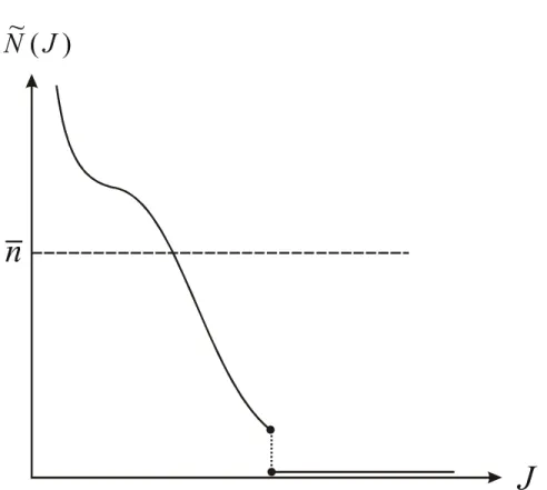
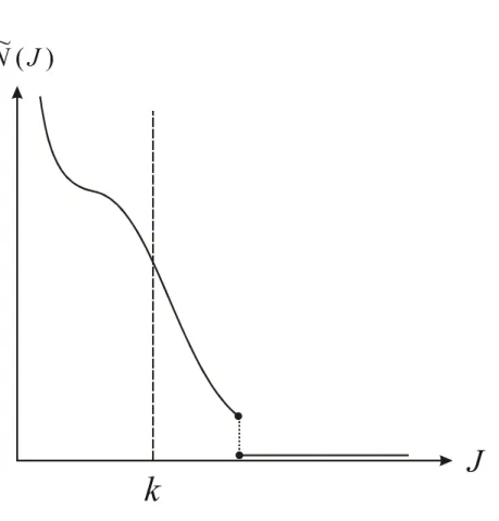
INSERT FIGURE 3 ABOUT HERE
The curve N˜(J) in Figure 3 can be interpreted as aggregate demand
for sellers by market makers; it is the convex hull of the correspondence
giving the value(s) ofnsolving the market maker’s problem taking as given
the price of sellers, J. It is downward sloping as the demand for sellers
decreases withJ. Without entry, J adjusts so that N˜(J) = ¯n; with entry,
we haveJ =kand the number of sellers adjusts. In Proposition 6 we show
that equilibrium without entry always exists andJ is uniquely determined.
With entry, equilibrium exists assuming γ is not too high, and if it exists
equilibrium is generically unique. The existence result is similar to what we found in previous models, but uniqueness here contrasts with the multiplicity
found under bargaining and price taking. Intuitively, it reflects the fact that market makers effectively internalize any strategic complementarity between money demand and entry.
Assuming the solution to (37) is unique, all open submarkets must have
the same(q, z, n). EliminatingJ from the constraint and using (38), we can
write (41) as
βn
γ z=g[q,1−η(n)], (42)
where g is defined in (17). Interestingly enough, (42) is the first order
condition from the generalized Nash problem where the seller’s bargaining
power is η(n); hence, in competitive search equilibrium the terms of trade
endogenously satisfy the Hosios condition.
PROPOSITION 7: With either n= ¯nor free-entry, the optimal policy
isγ=β and it implies equilibrium is unique and efficient.
PROOF: From (38), q =q∗ if and only if γ = β. From (35) and (42),
the free-entry condition is α(n)
n {g[q,1−η(n)]−c(q)}=k. (43)
Whenq =q∗, (43) yields
α0(n) [u(q∗)−c(q∗)] =k, (44)
where we have usedg[q∗,1−η(n)]−c(q∗) =η(n) [u(q∗)−c(q∗)]from (17).
Comparing (44) with (5), equilibrium is fully efficient if and only if γ =β.
Q.E.D.
If n = ¯n then equilibrium is efficient at the Friedman rule, basically
because there is no holdup problem. A close examination of (37) suggests that competitive search equilibrium is equivalent to having buyers and sellers
contract (commit to the terms of trade) before matching, which of course gets around the holdup problem. Hence competitive and competitive search
equilibrium both yield efficiency along the intensive margin. When n is
endogenous, competitive search equilibrium does more, because the Hosios condition arises endogenously; i.e. the extensive margin is also efficient at
γ=β because market makers internalize the effects ofnon arrival rates.
6. CONCLUSION
We considered three different market structures for monetary economies: search equilibrium (bargaining), competitive equilibrium (price taking), and competitive search equilibrium (price posting with directed search). We found that efficiency and the effects of policy depend crucially on the mar-ket structure. Table 1 shows the efficiency properties of the different models
at the Friedman rule. Regarding the intensive margin,γ=β impliesq=q∗
in competitive equilibrium and competitive search equilibrium, butq < q∗in
search equilibrium ifθ <1. Regarding the extensive margin,nis generically
inefficient in search equilibrium and competitive equilibrium, because these
mechanisms do not generally internalize the effects of entry; efficient n
re-quires the Hosios condition. In competitive search equilibrium the relevant
condition holds endogenously, sonas well asq are efficient at the Friedman
rule.
TABLE 1
SE CE CSE
Intensive margin q < q∗ ifθ <1 q=q∗ q=q∗
Table 2 shows the welfare effect of inflation forγ≈β. Withnexogenous,
inflation has only a second-order effect in competitive and competitive search
equilibrium, due the envelope theorem: W is maximized and ∂W/∂γ = 0
at γ = β. In the case of search equilibrium with θ < 1, however, the
envelope theorem does not apply: W is still maximized at γ = β, but
∂W/∂γ < 0 because we are at a corner solution (γ = β is the minimum inflation rate consistent with equilibrium). Inflation has afirst order effect in
this case. With nendogenous, inflation decreasesW in search equilibrium,
but has an ambiguous effect in competitive equilibrium; it is possible to have ∂W/∂γ > 0. Finally, in competitive search equilibrium the envelope
theorem applies to bothq andnwhennis endogenous, and so inflation has
only a second-order effect on welfare near the Friedman Rule.
TABLE 2
SE CE CSE
n exogenous ∂∂γW <0 ifθ <1 ∂∂γW ≈0 ∂∂γW ≈0
nendogenous ∂∂γW <0 ∂∂γW ≷0 ∂∂γW ≈0
One can ask about the quantitative implications of the results. In Ro-cheteau and Wright (2004) we numerically study the models analyzed here
by calibrating to standard data, and askinghow much the welfare effects of
inflation depend on the market structure.21 The findings are as follows. In
competitive search equilibrium our estimated welfare cost is very similar to
previous estimates, such as those in Lucas (2000): going from 10% to 0%
inflation is worth between 0.67% and 1.1% of consumption, depending on
details of the calibration. In search equilibrium, the estimated cost can be
2 1We actually work with a slightly different framework in that paper, where instead
of assuming afixed number of buyers and free entry by sellers we let each agent choose whether to be a buyer or a seller.
between3%and 5%, considerably bigger than what is found in most of the literature. In competitive equilibrium, the cost is somewhere between the
other two models; while it is possible for positive inflation to be optimal this
was not the case at the calibrated parameter values. While by no means
de-finitive, we think these results are suggestive, and that it is worth pursuing
further quantitative work on these models.
Research Department, Federal Reserve Bank of Cleveland, P.O. Box 6387, Cleveland, OH 44101-1387, U.S.A.; and Australian National Uni-versity; Guillaume.Rocheteau@clev.frb.org;
and
Department of Economics, University of Pennsylvania, 3718 Locust Walk, Philadelphia, PA 19104, U.S.A.; rwright@econ.upenn.edu.
References
Alvarez, F., and M. Veracierto (1999): “Labor Market Policies in an
Equi-librium Search Model,”NBER Macroeconomics Annual, 14, 265-304.
Berentsen, A., G. Rocheteau and S. Shi (2001): “Friedman Meets Hosios: Efficiency in Search Models of Money,” Unpublished Manuscript. Burdett, K., S. Shi, and R. Wright (2001): “Pricing and Matching with
Frictions,”Journal of Political Economy, 109, 1060-1085.
Camera, G., and D. Corbae (1999): “Money and Price Dispersion,”
Inter-national Economic Review, 40, 985-1008.
Corbae, D., T. Temzelides, and R. Wright (2003): “Directed Matching and
Monetary Exchange,”Econometrica, 71, 731-756.
Curtis, E., and R. Wright (2004): “Price Setting and Price Dispersion in a
Monetary Economy; Or, the Law of Two Prices,”Journal of Monetary
Economics,Forthcoming.
Diamond, P. A. (1982): “Aggregate Demand Management in Search
Equi-librium,”Journal of Political Economy, 90, 881-94.
– (1984): “Money in Search Equilibrium,” Econometrica, 52, 1-20.
Faig, M., and X. Huangfu (2004): “Competitive Search Equilibrium in Monetary Economies,” Unpublished Manuscript.
Green, E. J., and R. Zhou (1998): “A Rudimentary Random-Matching
Model with Divisible Money and Prices,”Journal of Economic Theory,
Hosios, A. J. (1990): “On the Efficiency of Matching and Related Models of
Search and Unemployment,” Review of Economic Studies, 57, 279-298.
Johri, A. (1999): “Search, Money and Prices,” International Economic
Review, 40, 439-54.
Kamiya, K., and T. Shimizu (2003): “Real Indeterminacy of Stationary Equilibria in Matching Models with Media of Exchange,” Unpublished Manuscript.
Khan, A., J. Thomas, and R. Wright (2004): “On the Distribution of Money Holdings in Search Equilibrium: Quantitative Theory and Pol-icy Analysis,” Unpublished Manuscript.
Kiyotaki, N., and R. Wright. (1989): “On Money as a Medium of
Ex-change,”Journal of Political Economy, 97, 927-954.
– (1991): “A Contribution to the Pure Theory of Money,” Journal of
Economic Theory, 53, 215-235.
– (1993): “A Search-Theoretic Approach to Monetary Economics,”
Amer-ican Economic Review, 83, 63-77.
Kocherlakota, N. R. (1998): “Money is Memory,” Journal of Economic
Theory, 81, 232-251.
Lagos, R., and G. Rocheteau (2003): “Output, Inflation and Welfare,”
Unpublished Manuscript.
Lagos, R., and R. Wright (2002): “A Unified Framework for Monetary
– (2003): “Dynamics, Cycles, and Sunspot Equilibria in ‘Genuinely
Dy-namic, Fundamentally Disaggregative’ Models of Money,”Journal of
Economic Theory, 109, 156-171.
Levine, D. (1991): “Asset Trading Mechanisms and Expansionary Policy,”
Journal of Economic Theory, 54, 148-164.
Li, V. (1995): “The Optimal Taxation of Fiat Money in Search
Equilib-rium,” International Economic Review, 36, 927-942.
Lucas, R. E. (2000): “Inflation and Welfare,”Econometrica, 68, 247-274.
Lucas, R. E., and E. C. Prescott (1974): “Equilibrium Search and
Unem-ployment,”Journal of Economic Theory, 7, 188-209.
Moen, E. R. (1997): “Competitive Search Equilibrium,”Journal of
Politi-cal Economy, 105, 385-411.
Molico, M. (1999): “The Distribution of Money and Prices in Search Equi-librium,” Unpublished Manuscript.
Mortensen, D. T., and C. A. Pissarides (1994): “Job Creation and Job
Destruction in the Theory of Unemployment,” Review of Economic
Studies, 61, 397-415.
Mortensen, D. T., and R. Wright (2002): “Competitive Pricing and
Ef-ficiency in Search Equilibrium,” International Economic Review, 43,
1-20.
Petrongolo, B., and C. A. Pissarides (2001): “Looking into the Black Box:
A Survey of the Matching Function,”Journal of Economic Literature,