Analysis of Public Expenditure on Health Using State Level Data

Analysis of public expenditure on

health using state level data

Ramesh Bhat

Nishant Jain

Doctoral Student, IIM Ahmedabad

Indian Institute of Management

Ahmedabad

2

Analysis of public expenditure on

health using State level data

Abstract

Increasingly the governments are facing pressures to increase budgetary allocations to social sectors. Recently there has been suggestion to increase the government budget allocations to health sector and increase it to 3 per cent of GDP. Is this feasible goal and in what time-frame? Health being State subject in India and much depends on the ability of the State governments to allocate higher budgetary support to health sector. This inter alia depends on what are current levels of spending, what target spending as per cent of income the States assume to spend on health and given fundamental

relationship between income levels and public expenditures, how fast expenditures can respond to rising income levels. We present analysis of public expenditures on health using state level public health expenditure data to provide preliminary analysis on these issues. The findings suggest that at state level governments have target of allocating only about 0.43 per cent of SGDP to health and medical care. This does not include the allocations received under central sponsored programmes such as family welfare. Given this level of spending at current levels and fiscal position of state governments the goal of spending 2 to 3 per cent of GDP on health looks very ambitious task. The analysis also suggests that elasticity of health expenditure when SGDP changes in only 0.68 which suggest that for every one percent increase in state per capita income the per capita public healthcare expenditure has increased by around 0.68 per cent.

Key words: Public expenditure on health, Elasticity of public health expenditures, Unit root, Panel GMM estimator

1.

Introduction

Increasingly the governments are facing pressures to increase the budgetary allocations to social sector. Recently there has been suggestion to increase the budget allocations to health sector and increase it to 3 per cent of GDP. Is this feasible goal? We

certainly need some understanding of the behaviour of public expenditures on health. Health is state subject in India and therefore analysis of public health expenditures by States assumes greater significance. The analysis of health care expenditures in general has been a topic of research and discussion in recent times globally. In particular, the relationship between the income and health care expenditure (HCE) has been focus of research for the reason that it helps us to understand the key determinants of

healthcare expenditures and also provides insights into linkages between income variable on the one hand, and demand and supply side of health on the other. Since in India we are talking about increasing the public expenditures on health to 3 per cent of GDP, this analysis would provide some insights into our proposed goal.

One of the areas of this analysis has been focus on understanding the income elasticity of health expenditures. This research has used standard demand theory framework. Since the seminal work of Newhouse (1977) which estimated the relationship between health care expenditure and gross domestic product (GDP), a large number of studies have been carried out to examine this relationship in different contexts and answer the question what makes health care expenditure to increase. We are asking similar

question in our context. What are necessary and sufficient conditions for public health expenditures to increase? One important determinant is income or GDP. Most of the studies on this topic have been carried out in developed country context. In some of those settings the health care costs have gone up significantly over the years and expenditure-income analysis provides some interesting insights into health policy issues. A number of studies agree that there is a relationship between GDP and HCE in various. These studies vary from country level analysis to a much-disaggregated

4 level like province or state level analysis. Most of the studies in this field have focused on health care expenditure including both private and public expenditures.

In India health is responsibility of State governments and therefore the budgets allocations of each State include the allocation to health sector programmes. Besides this State governments also receive support from central government through central sponsored programmes and various national programmes. In India the government budget allocations to health sector would reflect more of supply side factors than demand side. Whereas the private sector health care expenditures would represent more of demand side conditions than supply side. Hence, the analysis based on the combined expenditure may not be appropriate and may produce erroneous results. Moreover, by separately analysing them we get more insight into behaviour of

expenditures and their determinants. In this paper we focus on analysis of relationship between public healthcare expenditure and GDP using state level data.

2.

Context of study

Like in developed countries health care expenditure in India is also steadily increasing. However, public health expenditure has been grossly inadequate right from the 1940s. The government has been spending less than private expenditures on health. The Bhore Committee report stated that per capita private expenditure on health was Rs. 2.50 compared to a state per capita health expenditure of just Rs. 0.36 which is 1/7th _of

private expenditures. In the 1950s and 1960s private health expenditure was 83 per cent and 88 per cent of total health expenditure respectively1_{. Today also according to} latest figures the proportion of public expenditure on health to GDP in India is only 0.9 per cent of GDP while the average public spending of less-developed countries is 2.8 per cent of GDP. Only 17 per cent of all health expenditure in India is borne by the government, the rest being borne privately by the people, making it one of the most highly privatised healthcare systems of the world2_.

Within India also we see that there is huge gap in different states in economic terms and also in terms of development of health sector. Ahluwalia (2000) in his article raises this issue while analysing the performance of individual states. The paper states, “The

economic performance of the individual states in post-reforms period has received less attention than it deserves in the public debate on economic policy. There is very lively debate in the academic world and in the press on our national economic performance and the success or failure of various aspects of national policies, but there is relatively little analysis of how individual states have performed over time and the role of state government policy in determining state level performance.” We examine the state level public health expenditure. In fact state as unit of study needs to be studied because of the following structural and methodological reasons:

Structural and political issues

India is a federal democracy in which the constitutional division of powers between the centre and the states make the states pre-eminent in many areas and co-equal with centre in other areas. Health is State subject and state policies would have important bearing on the public health expenditures in India. Also nowadays government at the state level are run by different political parties and competition among them should make the performances of individual states a matter of high political and electoral interest. After liberalisation degree of control exercised by centre has been reduced in many areas leaving much greater scope for States to improve their performance level and initiatives. This is particularly true as far as attracting investments, both domestic and foreign, is concerned.

Methodological issues

Renenelt and Levine (1991) raise this question that what is the appropriate unit of study. In particular, are countries the appropriate unit to study, or should we conduct analysis at a more disaggregated level? Since countries are composed of states, any country’s growth rate will depend on the growth of its different states. A second issue with using country as a unit of study involves sampling. Regression analysis

presupposes that data has been taken from a single population. It is not clear, however, whether states are indeed drawn from same population3_{. Different Indian states can be}

a part of the same analysis because they have several factors in common. They are broadly governed by the same legal system; they have same broad health policy devised by the central government; and have same constitution. But there are also differences. The economic, social-cultural and political differences are there. Thus a study at the

6 state level not only provides an opportunity for analysis at disaggregate level but also allows the assumption of regression analysis to be maintained (e.g., data points should be from the same population).

3.

Literature Review

There is a large literature dealing with issues related to health care expenditure. If we observe closely we can divide this literature into following broad categories.

Studies related to relationship between health expenditure and income One important finding in earlier studies has been that the ratio of healthcare

expenditure to GDP increased as countries were getting developed economically and industrially. We can go to as back as in 1963 and 1967 when pioneering work of Abel-Smith brought out this issue in World Health Organisation studies. They found that after adjusting for inflation, exchange rates and population, GDP is a major

determinant of health expenditure.

In a seminal paper Newhouse (1977) raises the question what determines the quantity of resources any country devotes to medical care. The analysis provided suggests that per capita GDP of the country is the single most important factor affecting health expednitures. The study found a positive linear relationship between fraction of health care expenditure to GDP and GDP4_{. Results of Newhouse were consistent with an}

earlier study by Kleiman (1974) and both these papers worked as a base for a large literature, which viewed income as a major determinant of health care expenditure. This result was also verified by lots of studies later on.

Gerdtham et al. (1992) used a single cross section of nineteen OECD countries in 1987. They found per capita income, urbanisation, and the share of public financing to total health expenditure as positive and significant variables. Gbesemete and Gerdtham (1992) used a cross sectional sample of thirty African countries in 1984. They found that per capita GNP was the most significant factor in explaining per capita health care expenditure. Hitris and Posnett (1992) used 560 pooled time series and cross section observations from 20 OECD countries over the period 1960-1987 and found a strong

and positive correlation between per capita health spending and GDP. Later also many authors studied the performance of health expenditures. Most of the works of these authors were based on the relationship between health care expenditure and GDP. Some important works, which we can mention here, are Hansen and King (1996), McKoskey and Selden (1998), Gerdtham and Lothgren (2000), Karatzas (2000). All of these studies agreed that health care expenditure is dependent on GDP of the country. Another very important aspect, which different authors tried to explain, was that whether health care expenditure is a necessity good or luxury good.

Studies related to elasticity of health expenditure and income

Whether healthcare is a luxury or necessity is very important from the point of view estimating future expenditure on healthcare. This is so because if health care is a luxury product it will consume an ever-increasing share of national income. It also has

implications for the link between healthcare expenditure and economic well-being. Generally normal measures of health like infant mortality rate, death rate, morbidity etc. are more or less not very different for similar kind of countries (for example in OECD countries). But health care spending may differ more than these normal measures. There can be a case that marginal utility of health care expenditure can be very low. This comes out from the Engel’s curve5 _{and Engel’s law}6_.

Newhouse (1977) argued that since the income elasticity of health care expenditure is greater than 1 therefore it could be treated as a “luxury” good. This raised a major debate in the literature that whether health care is luxury or necessity. Literature gives a contrasting view of the elasticity of health care expenditure with respect to income. Some studies (like Newhouse, 1977; Gerdtham et al., 1992) found the elasticity greater than one while many other studies (Manning et al., 1987; McLaughlin, 1987; Di Matteo and Di Matteo, 1998) found elasticity much less than one. Getzen (2000) in his paper analyses the literature and concludes that health care is neither “a necessity” nor “a luxury” but “both” since the income elasticity varies with the level of analysis. With insurance individual income elasticities are typically near zero while that of nations is

8 mostly more than one. Getzen (2000, Exhibit 1)7 _{provides a summary of the work} done in calculating the elasticity of health expenditure and GDP by the level of

aggregation. In general higher the level of aggregation higher is the income elasticity of health care expenditure. However, the empirical evidence does not sustain this claim. A possible explanation for this result is the presence of an aggregation problem, in the sense that most of the studies in this area have focused exclusively on the analysis of health expenditures. If we segregate both private and public healthcare expenditure and then try to calculate their elasticity then may be some more clarity will come on this issue.

Studies on issues of stationarity and cointegration

Many authors have studied performance of health function with majority of the work is based on the relationship between health care expenditure and the GDP. Most of these studies use time series data. Here we have to see that variables, which have been used, may not be stationary. Therefore, the estimated relationships may be spurious. Before estimating the relationship many studies have focused on first examining the stationarity of the time series used in analysis. Following this many studies have found that the time series under consideration are generally not stationary. So the studies have used cointegration approach. A number of studies have been carried out using the cointegration approach. But there is no unanimity between researchers regarding presence of cointegration between health expenditures and income.

Contradictory results have been found by the authors. Gerdtham and Lothgren (2000) have made an attempt to examine these contradictions. They showed that different conclusions regarding stationarity and cointegration between health expenditure and income in the previous studies were dependent on whether those studies were

conducted on individual or pooled series and also whether time trends were included in the estimations. Finally, they conclude that health expenditures and income for a panel of OECD countries have unit roots and they are cointegrated. Gertham and Lothgren did not, however, follow up their cointegration tests with estimates of elasticity of health care expenditure with respect to income (GDP), and so did not address the question of health’s status as a luxury or necessity good. However, results

of Gerdtham and Lothgren are not entirely free from criticism as shown by Taylor and Sarno (1998) or Banerjee et al. (2000).

Studies related to use of Panel Data

Initial studies used cross-sectional or time series data for the analysis. In more recent studies researchers (e.g. Gerdtham 1992, Hitris and Posnett 1992, Gertham et al. 1995, Getzen 2000) have used panel data. Panel data sets for economic research possess several major advantages over conventional cross-sectional or time-series data sets (e.g., Hsiao (1985a, 1995, 2000)). Main advantages of panel data are that they usually give a large number of data points, increasing the degree of freedom and reducing the collinearity among explanatory variables – hence improving the efficiency of econometric estimates. Longitudinal data allows analysing a number of important economic questions that cannot be addressed using cross-sectional or time series data sets, especially properties related to states and time specific effects. The use of panel data also provides a means of resolving or reducing the magnitude of the problem of presence of omitted (unmeasured or unobserved) variables that are correlated with explanatory variables.

Although panel data has many advantages, a problem can arise if several trending variables are present in panel data regressions for example health expenditure and GDP. Philips (1986) showed that regressions involving non-stationary variables might lead to spurious results showing apparently significant relationships even if variables are generated independently. However, if the variables are cointegrated the ordinary regression estimators turn out to be super consistent (Engle and Granger 1987). Studies related to health financing in India

In India there are few studies which have touched upon the issue of healthcare

financing and its nature. First study was R.B. Lal’s Singpur study of private household expenditure, which talked about private expenditure on health in Singpur area and also what was the government healthcare expenditure for the same area (GOI, 1946). The Indian Institute of Management, Ahmedabad had carried out a study of health finance covering all the levels of health expenditure – state, municipal, corporate and

10 Roger Jefferey. He looked at state health expenditure from the perspective of planning – the administrative process involved in making allocations – and in context of policy changes. Tulasidhar and Sarma (1993) did a comparative study of different states of India with respect to public expenditure, medical care at birth and infant mortality. They found that in all the states per capita real public spending grew faster than real per capita state domestic product. Recently a number of studies have been done on the healthcare financing in India. Duggal (1996) discusses the public-private participation in health sector and how this can be optimised for best results. Bhat (1996, 2000) discusses about the importance of regulating the private sector in India and how public-private partnership can bring needed resources while also taking care that the

vulnerable groups – the poor and rural populations – have access to health facilities. These studies suggest that India’s dependence on private sector in healthcare is very high. Utilisation studies show that a third of in-patients and three fourths of out-patients utilise private healthcare facilities (Duggal and Amin 1989; Yesudian 1990; Visaria and Gumber 1994).

Dreze and Sen (1995) analysed life expectations at birth and they found substantial differences at birth across states Rajasthan have infant and socio-economic groupings. States such as Madhya Pradesh, Orissa have mortality rates of well over 100 per 1000 live births in rural areas (Dreze and Sen 1995; Mahal, Srivastava and Sanan 2000). In another study Mahal et al. (2000) tried to find the distribution of public health subsidies in India in different states. Despite a considerable desire for “equity” in public policy documents, they found that public subsidies on health are distributed quite unequally across different socio-economic groups in India. At the all-India level, the share of the richest 20 per cent of the population in total public sector subsidies is nearly 31 per cent, nearly three times the share of the poorest 20 per cent of the population. In rural areas this inequality was much greater where the share of the top 20 per cent in public subsidies was nearly four times that of the poorest 20 per cent. Mahal et al. (2000) find that 31 per cent of public subsidies on health accrued to urban residents, somewhat higher than their share in the total population of about 25 per cent. If we look at the state level then there also they found substantial differences in

the degree of inequality, with southern states such as Kerala, Tamilnadu and Andhra Pradesh, and the western states of Maharashtra and Gujarat enjoying a much more equal distribution than the north Indian states. Some of this inequality in the

allocation of public health subsidies can be explained by income-related differences in utilisation patterns of public facilities, with the rich using more care, if health care is a normal good. But if, however, promoting equity is a key objective of the state, there is no doubt that substantial scope for improvement remains, whether in terms of inter-state equity, or within inter-state distributions of public subsidies.

Studies at state level of India

There are very few studies, which takes states of India as the unit of analysis. For example, Mitra and Varoudakis (2002) examined the effects of infrastructure on manufacturing industries’ total factor productivity and technical efficiency in the case of Indian states. They showed that differences in infrastructure endowments across Indian states explain in a significant way their differences in industrial performances. In another study, Datt and Ravallion (1998) study the rural poverty elimination in

different states of India. They found that speed of rural poverty elimination has been diverse across different states. But there are very few studies of this kind.

4.

Healthcare expenditure in India

The Indian constitution charges the states with "the raising of the level of nutrition and the standard of living of its people and the improvement of public health" (see The Constitutional Framework, Ch. 8). Central government efforts at influencing public health have focused on the five-year plans, on coordinated planning with the states, and on sponsoring major national health programs. For most national health programmes government expenditures are jointly shared by the central and state governments. Healthcare expenditure is a very necessary social expenditure for any country. Like any other social expenditure health expenditure also requires a significant contribution from the Government. Whether it is a developed country or a developing one state’s role in developing a good health infrastructure and assuring good health to everybody becomes very critical and important. The spending on health has major contributions coming from private households (75 per cent). State governments contribute 15.2

12 percent, the central government 5.2 percent, third-party insurance and employers 3.3 percent, and municipal government and foreign donors about 1.3 (World bank 1995). Of these proportions, 58.7 percent goes toward primary health care (curative,

preventive, and promotive) and 38.8 percent is spent on secondary and tertiary inpatient care. The rest goes for non-service costs. Table 1 provides comparison of public expenditures on health of various countries.

Table 1: Public expenditure on health

as % of total expenditure on health, 20018

The comparison of health expenditure with other countries suggests that India’s public health expenditure is only 17.9 per cent of total expenditure on health care while it is close to 90 per cent for smaller countries like Bhutan and Maldives.

Centre and state roles in public healthcare expenditures

The total public health care expenditure is composed of state level allocations and allocations from central government. The central sponsored programmes have been one key policy initiative of the Government of India to support the health sector programmes directly. The centre provides direct and partial (matching grant) support to the states in meeting both recurring and non-recurring expenditure of programmes under this policy initiative. The states’ share in the total revenue expenditure has been declining. This is also reflection of the fact that state governments are going through serious fiscal problems. The role of central support in state budgetary allocations is increasing. We can see from the following graphs that the percentage of State expenditure is decreasing in total health expenditure and the same is rising of central

Country Percentage

Bhutan 90.6

Maldives 83.5

Democratic People's Republic of Korea 73.4

Timor-Leste 59.5 Thailand 57.1 Sri Lanka 48.9 Bangladesh 44.2 Nepal 29.7 Indonesia 25.1 India 17.9 Myanmar 17.8

govt. expenditure, though the change is not very much in percentage terms (see Figures 1 and 2).

Percentage of Central Govt. in Total Revenue Expenditure

on Health 6.00% 7.00% 8.00% 9.00% 10.00% 11.00% 12.00% 13.00% 14.00% 1987 1988 1989 1990 1991 1992 1993 1994 1995 1996 1997 1998 1999 2000 2001 2002 2003 0 2 0 0 0 4 0 0 0 6 0 0 0 8 0 0 0 1 0 0 0 0 1 2 0 0 0 1 4 0 0 0 1 6 0 0 0 1 8 0 0 0 1 9 8 7 1 9 8 8 1 9 8 9 1 9 9 0 1 9 9 1 1 9 9 2 1 9 9 3 1 9 9 4 1 9 9 5 1 9 9 6 1 9 9 7 1 9 9 8 1 9 9 9 2 0 0 0 2 0 0 1 2 0 0 2 2 0 0 3 T o ta l R e v. E x p . O n H e a lth C e tra l G o v t. R e v . E x p . O n H e a lth

Figure 2: Central Govt. Rev. Exp. On Health Figure 1: State Govt. Rev. Exp. On Health

0 2 0 0 0 4 0 0 0 6 0 0 0 8 0 0 0 1 0 0 0 0 1 2 0 0 0 1 4 0 0 0 1 6 0 0 0 1 8 0 0 0 1 9 8 7 1 9 8 8 1 9 8 9 1 9 9 0 1 9 9 1 1 9 9 2 1 9 9 3 1 9 9 4 1 9 9 5 1 9 9 6 1 9 9 7 1 9 9 8 1 9 9 9 2 0 0 0 2 0 0 1 2 0 0 2 2 0 0 3 T o t a l R e v . E x p . o n H e a l t h S t a t e G o v t . R e v . E x p . o n H e a l t h

Percentage of State Govt. in Total Revenue Expenditure

on Health 86.00% 87.00% 88.00% 89.00% 90.00% 91.00% 92.00% 93.00% 94.00% 1987 1988 1989 1990 1991 1992 1993 1994 1995 1996 1997 1998 1999 2000 2001 2002 2003

14 As compared to these allocations, the private expenditure on healthcare is increasing. In fact in the past five six years it has grown exponentially. From just Rs. 195 billion in 1994 it rose by more than five times to Rs. 1283 billion in 2003 (see Figure 3).

Figure 3: Private Final Consumption on Health

Private Final Consumption on Health 0 20000 40000 60000 80000 100000 120000 140000 1987 1988 1989 1990 1991 1992 1993 1994 1995 1996 1997 1998 1999 2000 2001 2002 2003 Year V a lu e (Rs . Cro re)

Trend of public healthcare expenditure at state level

Per capita public healthcare expenditure in different states in India does not show any trend, expect in two states: Punjab and Kerala. State government revenue expenditure for medical and healthcare increased from just around Rs. 50 billion in 1992 to more than 150 billion in 2001, an increase of more than three times in a decade (see Figure 5). One observation, which we can easily make by analysing Figure 4, is that around 1996 there was a sharp dip in public healthcare expenditures (PHCE) across all states (as shown by dotted line is Figure 4). After that PHCE again rose. Best example of this we can see in Punjab and Andhra Pradesh states. Bihar and UP two backward but one of the largest states shows that here also they have one of the lowest PHCE among all states consistently, even smaller states like Kerala and Assam spends more than these two states. One reason of this can be that these two are one of the poorest states. States like Tamilnadu, Rajasthan and Maharashtra does not show much fluctuation in

PHCE. So broadly from the above graph we get the picture that PHCE does not vary much in time in different states.

Figure 4: Public Health Care Expenditure per capita Andhra Pradesh Assam Bihar Gujarat Karnataka Kerala Madhya Pradesh Maharashtra Orissa Punjab Rajasthan Tamil Nadu Uttar Pradesh West Bengal 0 20 40 60 80 100 120 140 160 1990 1991 1992 1993 1994 1995 1996 1997 1998 1999 2000 2001 2002 Year Va lu e ( R s. C ror e)

parts, from 1990 to 1996 and from 1996 to 2002, then we can actually try to see that by what extent PHCE varied in these two time periods and also for the whole time period. This analysis is presented in Table 2.

Table 2: Growth of Public Healthcare Expenditure (PHCE) Per Capita (in real terms)

Change* Percentage Change

1990-1996 1996-2002 1990-2002 1990-1996 1996-2002 1990-2002 Andhra Pradesh -211.1 263.4 52.3 -28.16% 48.92% 06.98% Assam 3.4 -15.5 -12.1 00.56% -02.56% -02.01% Bihar -111.7 160 48.2 -26.25% 50.96% 11.33% Gujarat -156.6 110.3 -46.3 -17.48% 14.91% -05.17% Karnataka -103.6 270.3 166.7 -13.23% 39.79% 21.30% Kerala -73.2 172.2 99.1 -07.99% 20.43% 10.81% Madhya Pradesh -103.6 161.1 57.5 -18.54% 35.41% 10.30% Maharashtra -144.2 278.3 134.1 -16.80% 38.97% 15.62% Orissa -186.9 154.3 -32.6 -30.32% 35.92% -05.29% Punjab -414.9 583.8 168.9 -33.29% 70.20% 13.55% Rajasthan -86.7 152.1 65.5 -10.95% 21.60% 08.28% Tamilnadu -44.6 134.5 89.9 -05.07% 16.09% 10.20% Uttar Pradesh -160 -5.3 -165.2 -26.40% -01.18% -27.27% West Bengal -35.5 251.8 216.3 -05.69% 42.76% 34.64%

All India (States) -107.8 160.8 53.1 -14.90% 26.14% 07.34%

* Figures are in Rs. millions

From the above table few interesting point emerges. We see here that public health expenditure (PHCE) in real terms of all the states except Assam went down in the period 1990-96 but it increased during the period 1996-2002 for all states except Uttar Pradesh and Assam. Overall in this period PHCE increased for most of the states except Assam, Gujarat, Orissa and Uttar Pradesh.

But if we observe per capita health expenditure as a percentage of per capita Gross SDP (both in real terms) for the same period of time a different picture emerges. The percentage spending of state governments shows a declining trend (see Figure 5).

Figure 5: PHCE to GSDP Ratio Andhra Pradesh Assam Bihar Gujarat Kerala Kerala Madhya Pradesh Maharashtra Orissa Punjab Rajasthan Tamil Nadu Uttar Pradesh West Bengal 0 0.002 0.004 0.006 0.008 0.01 0.012 0.014 1990 1991 1992 1993 1994 1995 1996 1997 1998 1999 2000 2001 2002 Year Ra ti o

Pradesh does not fare very badly here. In fact Bihar comes across as one of the state with highest ratio. Here big states like Maharashtra, Madhya Pradesh, Gujarat comes have not done well. States like Bihar, Assam, Andhra Pradesh and Punjab shows very high fluctuation in PHCE to GSDP ratio while some states like Maharashtra and Gujarat does not show much fluctuation. We also see that that in 1996 there is a blip but this must be the result of fall in PHCE in 1996. One thing which comes out from the above figure is that in almost all the states PHCE as a percentage of GSDP has not increased much during past decade. During the period 1994 to 2002 health care

expenditure as a percentage of Gross SDP had in fact showing a declining trend. Keeping in mind the sharp dip in 1996 if we divide the period being studied into two parts, from 1990 to 1996 and from 1996 to 2002, then we can actually try to see that to what extent PHCE as a percentage of GSDP varied in these two time periods and also for the whole time period (see Table 3).

Table 3: Per cent change in PHCE/ GSDP ratio

1990-1996 1996-2002 1990-2002 Andhra Pradesh -40.51% 16.46% -30.72% Assam -05.79% -06.55% -11.96% Bihar -19.21% -05.14% -23.36% Gujarat -38.11% -07.95% -43.03% Karnataka -31.08% -00.33% -31.31% Kerala -31.20% -05.61% -35.07% Madhya Pradesh -31.14% 18.24% -18.58% Maharashtra -37.15% 21.36% -23.72% Orissa -31.53% 16.30% -20.37% Punjab -40.24% 44.05% -13.91% Rajasthan -26.81% -00.74% -27.35% Tamilnadu -30.40% -11.56% -38.45% Uttar Pradesh -28.96% -12.90% -38.12% West Bengal -25.90% 03.49% -23.31%

From the above table we can see that for all the states PHCE as a percentage of GSDP went down significantly in the period 1990-1996, for the period 1996-2002 again it went down except for Andhra Pradesh, Madhya Pradesh, Maharashtra, Orissa, Punjab and West Bengal. But on the whole for entire period it went down for all the states.

20 From this a very important point emerges that government priority for health care expenditure is decreasing over the years in all the states which means that less and less money per capita is being spent by government on healthcare as a percentage of income (see Figure 6).

The percentages decreases can be summarised as follows: % Decrease (1990-2002) States

More than 40% Gujarat

Between 30-40% Andhra Pradesh, Karnataka, Kerala, Uttar Pradesh, Tamilnadu Between 20-30% Orissa, West Bengal, Bihar, Maharashtra, Rajasthan

Less than 20% Madhya Pradesh, Punjab, Assam

From the above table some interesting point emerges. Gujarat has maximum decrease in HCE as a percentage of income. After that most of the southern states and Uttar Pradesh showed decrease in the ratio. In the next category are eastern states and western states. -11.96% -13.91% -18.58% -20.37% -23.31% -23.36% -23.72% -27.35% -30.72% -31.31% -35.07% -38.12% -38.45% -43.03% -50.00% -45.00% -40.00% -35.00% -30.00% -25.00% -20.00% -15.00% -10.00% -5.00% 0.00% 1 States Percentage Decrease Gujarat Tamilnadu Uttar Pradesh Kerala Karnataka Andhra Pradesh Rajasthan Maharashtra Bihar West Bengal Orissa Madhya Pradesh Punjab Assam

Figure 6: Percentage Decrease in PHCE - GSDP Ratio

Now from the above analysis a very important question emerges that why till 1996 HCE was decreasing at a rapid rate and after that it increased again somewhat. Selvaraju (2000) discusses about data till 1996 and he says that from 1990 to 1996 there was a period of contraction on expenditure. India started liberalisation and new economic policy in 1991 and at that point of time economic situation of country was in very bad state. Therefore, due to fiscal pressures the expenditures got affected and healthcare expenditure was no exception of that. But after 1996 again the situation improved and then that expenditure contraction period got over.

5.

Methodology and data

In order to estimate the relationship between income and public health care

expenditure we use real per capita gross state domestic product (GSDP) to represent income and real per capita state public health expenditure (PHCE) on health. For the purpose of analysis, health care expenditure refers mainly to expenditure incurred by states and does not include allocation of family welfare programme which is central sponsored programme. The expenditure on health does not include water supply and sanitation. We are, therefore, considering here only public health care expenditure. The data has been collected for each state. For the purpose of this study we have included 14 states in our analysis. The states included here account for more than 90 percent of the total population of country. The states included in the study are: Andhra Pradesh, Assam, Bihar, Gujarat, Karnataka, Kerala, Madhya Pradesh,

Maharashtra, Orissa, Punjab, Rajasthan, Tamilnadu, Uttar Pradesh, and West Bengal9_. We are taking time period from 1990 to 2002 for the purpose of analysis. Data from various sources was collected for this purpose. Main sources were database maintained by Centre for Monitoring Indian Economy (CMIE) and different Government publications. Expenditure in real terms has been used for all the analysis. Testing stationarity

Since we are using time series of income and health expenditure, the non-stationarity of the series can pose problems. First step is to test that whether data is stationary or not. To check whether the data is stationary or not first step is to plot the data and observe how it behaves. We plot GSDP and PHCE of all fourteen states and see that how it

22 behaves (See Figures 8 and 9). These plots give a rough idea that how these variables are behaving across different states. From Figure 8 we can see that GSDP shows upwards trend for all the states, which is expected also because we expect income to grow. While modelling the data we need to take into account this characteristic. But in Figure 9 we can see that there is no trend as such in PHCE.

For using time series data test of unit rot is very important for testing stationarity. Here we are using panel data which is nothing but time series data for number of states so we will be using panel unit root tests. For time series data testing for unit root is quite common now and there are lots of tests available for doing this. But testing unit root in panel data is a recent phenomenon. Levin and Li (1993) gave test for unit root in panel data but this and other tests of that time involved too restrictive assumptions on the slope parameters of pooled regressions. Now there are more flexible tests available like IPS test (Im et. al. 1997) and MW test (Maddala and Wu 1999) based on the Augmented Dickey-Fuller (ADF) equation.

The standard approach to test for non-stationarity of each observed time-series y observed over T time periods in a panel of is 1, . . . N, states is to estimate an Augmented Dickey–Fuller (ADF) regression here including a time trend:

∑ =

+

∆

+

+

+

=

∆

y

y

y

ρ

ε

β

δ

α

where

∆

y

=

y

−

y

residuals serially uncorrelated. The null hypothesis H0: βi = 0, that the data generating

process for the series for panel group i can be characterised as a difference stationary I (1) process, are tested against the trend stationary alternative H1: βi < 0 based on the

t-statistic of the βi estimate see, e.g., Campbell and Perron, 1991 and Hamilton, 1994 for

thorough treatments of the univariate unit root tests.

Since unit root tests are known to have low power in distinguishing between the non-stationary null and a non-stationary but persistent alternative, testing the individual state

series with only nine years of annual data the parameters of ADF equation will not give precise measures.

Using the cross-section dimension of data can increase the power of unit rot test. Im et al. treated data as N independent perhaps homogenous processes that either contain unit root or not. Thus, as the time and the cross-section dimension increase, unit root test statistics can be derived that converge to normally distributed variables (Freeman, 2003). Im et al. proposed an approach to perform unit root tests for panel data10

Another test, which was performed, for unit root is MW (Maddala and Wu 1999) based on ADF equation11_{. If the two series have unit root and it is of the same order then the} next step is to test for cointegration. But if both the series does not show unit root then there is no need to test for cointegration.

Computing elasticity

As concerning the effect of per capita income, one major question of health economics (and applied econometrics) is the estimation of health care expenditure income

elasticity. From the literature per capita public healthcare expenditure by state governments is assumed to be a function of per capita gross state domestic product. The model is specified in log-log form so that the coefficient estimates are elasticity and therefore enable us to interpret the relationship of health care expenditures and

income. We use the following model to estimate this relationship:

ln PHCEit = α + β₁*ln SGDPit + ε

where β1 will give the elasticity of PHCE with SGDP and ε is the residual.

Method of estimation

Another very important consideration in analysis of panel data is that whether it is a fixed effect (FE) model or a random effect (RE) model. The fixed effects model is a reasonable approach when we can be confident that the differences between units can be viewed as parametric shifts of the regression function. This model might be viewed as applying only to the cross-sectional units in the study, not to additional ones outside

24 the sample. For example, an inter-country comparison may well include the full set of countries for which it is reasonable to assume that the model is constant. In other settings, it might be more appropriate to view individual specific constant terms as randomly distributed across cross-sectional units. This would be appropriate if we believed that sampled cross-sectional units were drawn from a large population.

The generally accepted way of choosing between fixed and random effects is running a Hausman test. The Hausman test checks a more efficient model against a less efficient but consistent model to make sure that the more efficient model also gives consistent results.

Given a model and data in which fixed effects estimation would be appropriate, a Hausman test tests whether random effects estimation would be almost as good. In a fixed-effects kind of case, the Hausman test is a test of H0: that random effect would be

consistent and efficient, versus H1: that random effect would be inconsistent. (Note

that fixed effects would certainly be consistent.) The result of the test is a vector of dimension k (dim(b)) which will be distributed chi-square. So if the Hausman test statistic is large, one must use FE. If the statistic is small, one uses random effect model.

6.

Results

Unit root and Stationarity tests

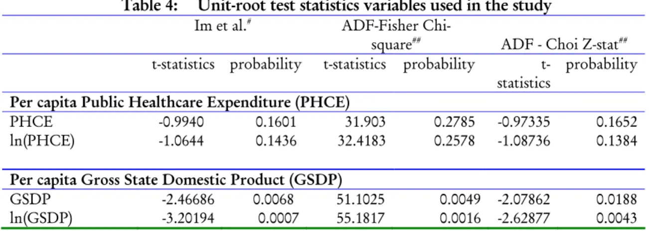
Unit root tests were done on both ln PHCE and ln GSDP separately (see Table 4). Table 4: Unit-root test statistics variables used in the study

Im et al.# _ADF-Fisher

Chi-square## _{ADF - Choi Z-stat}##

t-statistics probability t-statistics probability

t-statistics probability

Per capita Public Healthcare Expenditure (PHCE)

PHCE -0.9940 0.1601 31.903 0.2785 -0.97335 0.1652

ln(PHCE) -1.0644 0.1436 32.4183 0.2578 -1.08736 0.1384

Per capita Gross State Domestic Product (GSDP)

GSDP -2.46686 0.0068 51.1025 0.0049 -2.07862 0.0188

Im et al. test and ADF test statistics for PHCE has been estimated with constant and for GSDP with constant and trend.

# _{Probabilities are computed assuming asympotic normality,} ## _{Probabilities for Fisher tests are}

computed using an asympotic Chi-square distribution. All other tests assume asymptotic normality.

While estimating presence of unit root in PHCE we used constant and it was found that PHCE does not show presence of unit root. In both the tests i.e., Im et al. and ADF unit rot was not found. This means that real per capita public health care expenditure is stationary.

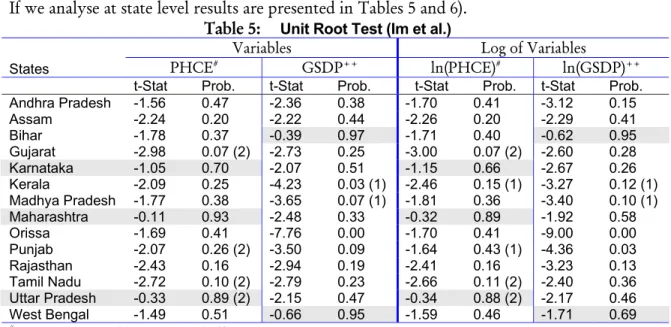
We can observe from the Figure 9 that GSDP shows presence of trend, therefore while estimating unit root in GSDP we estimate it in presence of constant and trend. Here also we see that we do not find evidence of unit root by both Im et al. and ADF tests. Therefore we can say that real per capita gross state domestic product is stationary. If we analyse at state level results are presented in Tables 5 and 6).

Table 5: Unit Root Test (Im et al.)

Variables Log of Variables

States PHCE# GSDP++ ln(PHCE)# ln(GSDP)++

t-Stat Prob. t-Stat Prob. t-Stat Prob. t-Stat Prob.

Andhra Pradesh -1.56 0.47 -2.36 0.38 -1.70 0.41 -3.12 0.15 Assam -2.24 0.20 -2.22 0.44 -2.26 0.20 -2.29 0.41 Bihar -1.78 0.37 -0.39 0.97 -1.71 0.40 -0.62 0.95 Gujarat -2.98 0.07 (2) -2.73 0.25 -3.00 0.07 (2) -2.60 0.28 Karnataka -1.05 0.70 -2.07 0.51 -1.15 0.66 -2.67 0.26 Kerala -2.09 0.25 -4.23 0.03 (1) -2.46 0.15 (1) -3.27 0.12 (1) Madhya Pradesh -1.77 0.38 -3.65 0.07 (1) -1.81 0.36 -3.40 0.10 (1) Maharashtra -0.11 0.93 -2.48 0.33 -0.32 0.89 -1.92 0.58 Orissa -1.69 0.41 -7.76 0.00 -1.70 0.41 -9.00 0.00 Punjab -2.07 0.26 (2) -3.50 0.09 -1.64 0.43 (1) -4.36 0.03 Rajasthan -2.43 0.16 -2.94 0.19 -2.41 0.16 -3.23 0.13 Tamil Nadu -2.72 0.10 (2) -2.79 0.23 -2.66 0.11 (2) -2.40 0.36 Uttar Pradesh -0.33 0.89 (2) -2.15 0.47 -0.34 0.88 (2) -2.17 0.46 West Bengal -1.49 0.51 -0.66 0.95 -1.59 0.46 -1.71 0.69

# _{Exogenous variables: Individual effects}

++_{Exogenous variables: Individual effects, individual linear trends; Figures in bracket shows number of lags}

Table 6: Unit Root Test (ADF)

Variables Log of Variables

States PHCE# GSDP++

ln(PHCE)

# ln(GSDP)

+ +

26

Prob. Prob. Prob. Prob.

Andhra Pradesh 0.47 0.38 0.41 0.15 Assam 0.20 0.44 0.20 0.41 Bihar 0.37 0.97 0.40 0.96 Gujarat 0.07 0.24 0.07 0.29 Karnataka 0.70 0.51 0.66 0.27 Kerala 0.25 0.03 0.15 0.12 Madhya Pradesh 0.38 0.07 0.36 0.10 Maharashtra 0.93 0.33 0.90 0.58 Orissa 0.41 0.00 0.40 0.00 Punjab 0.26 0.09 0.43 0.02 Rajasthan 0.16 0.19 0.16 0.13 Tamil Nadu 0.10 0.23 0.11 0.36 Uttar Pradesh 0.89 0.48 0.89 0.46 West Bengal 0.51 0.95 0.46 0.68

# _{Exogenous variables: Individual effects}

++_{Exogenous variables: Individual effects, individual linear trends}

Figures in bracket shows number of lags

From the above tables we can see that for PHCE Karnataka, Maharashtra and Uttar Pradesh shows presence of Unit root while for GSDP Bihar, and West Bengal shows presence of unit root. Since both these series are stationary then there is no need to test for cointegration.

Elasticity Computation

It is also necessary to see that whether it is a fixed model or random model. Hausman test was used to determine that whether it is a fixed or random model.

Table 7: Estimation of elasticity using Panel Data Methods

Model Constant Variable t-value R2

OLS Without Group Dummy Variables -1.649 0.653 18.144 0.646 Least Squares with Group and Period

Effects -2.207 0.714 07.023 0.918

Random Effects Model -1.932 0.684 0.830

Hausman Test * _0.14

* _{Hausman test favours Random Effect Model}

Three different models were used to calculate elasticity. From the Hausman test (H-value 0.14) it was found that Random Effect model is appropriate for this case. But we

see here that we did not found much difference between the coefficients of GSDP in all the three models. Elasticity calculated by this method comes between 0.65 and 0.71 (see Table 7).

If we analyse at state level and the results are presented in Table 8.: Table 8: Elasticity estimates of individual states

State Constant Variable t-value Adj. R2 _F-Value

Andhra Pradesh 2.19 0.23 1.63 0.017 1.20 Assam 11.07 -0.79 -1.47 -0.044 0.49 Bihar 1.25 0.30 0.93 -0.664 0.25 Gujarat 1.50 0.32 2.17 0.142 2.98 Karnataka 1.20 0.35 4.10 0.297 6.07 Kerala 2.54 0.22 1.80 0.084 2.10 Madhya Pradesh 0.30 0.42 2.49 0.082 2.07 Maharashtra 2.79 0.17 1.22 0.004 1.04 Orissa 3.83 0.02 0.09 -0.091 0.00 Punjab -4.15 0.93 2.39 0.178 3.60 Rajasthan 2.70 0.19 1.83 0.032 1.40 Tamil Nadu 3.28 0.14 2.48 0.106 2.42 Uttar Pradesh 24.52 -2.36 -6.41 0.660 24.30 West Bengal -0.39 0.52 3.58 0.386 8.53

White heteroscedasticity robust covariance matrix

7.

Target health expenditure of states

The analysis presented in previous section suggests that for every one per cent increase in state per capita income, the state level health expenditure has gone up by 0.684 per cent. Keeping this in view we would like to estimate what target PHCE/GSDP ratio states follow. We use the methodology of adaptive expectation model and estimate that what is the targeted ratio of health expenditure as percent of GDP which governments incur on healthcare.

Expectations are often important in economic models of dynamic processes, particularly in macroeconomic models, and finding ways to model them is often an important and difficult task for the applied economist using time series data. The adaptive expectations model has been one of the earliest approaches developed for this

28 purpose. Suppose that one hypothesise that target public health expenditure (PHCE*_)at time t is related to SGDP as follows:

PHCE* = β0 + β1SGDPt + µt

where β1 is target ratio of health spending as percent of SGDP. One assumes that states are not spending exactly as per this ratio. It aims to achieve this target over period of time with some speed of adjustment. This can be modeled as follows:

(PHCEt – PHCEt-1) = δ (PHCEt* - PHCEt-1)

Simplifying this equation and substituting the value of PHCE* _{in above equation gives}

us the following equation:

PHCEt = δ PHCEt* + (1-δ) PHCEt-1

PHCEt = δβ0 + δβ1SGDPt + (1-δ) PHCEt-1 + δµt

PHCEt = α0 + α1SGDPt + α2 PHCEt-1 + εt

From the above we can estimate the elasticity as follows: β1 = α1 / (1-α2)

Where β1 is target of SGDP which should be spent on PHCE.

The estimation of above model using panel data poses some methodological problem. Though the panel estimation through fixed effect model and random effect model control for unobservable heterogeneity, because the specification of model is dynamic as it has lagged dependent variable as independent variable. The presence of lagged dependent variable on right hand side causes considerable difficulty in estimation as the error term may be auto-correlated; but more seriously, the lagged dependent variable is correlated with the error term when we use fixed or random effects models (Greene, 2003). The literature has suggested the use of instrumental variables (IV) estimators and panel generalized method of moments (GMM) estimator in estimation of dynamic models. Here to avoid the problems of heterogeneity and the biases caused by the lagged dependent variable, we use the panel GMM procedure based on Arellano and

Bond (1991) and Arellano and Bover (1995). The panel GMM estimator uses

instrument variables. In our estimations, we use as instruments for lagged dependent right-hand side variable. The results of the GMM estimator based on Arellano and Bover (1995) are given in Table 9. Estimation based on Arellano and Bover (1995) uses orthogonal deviations and it removes the individual effects.

Table 9: Estimation of target spending on health using Panel Generalized Methods of Moments estimation

Variables Coefficient t-Ratio#

PHCEt-1 _{0.548750 13.81}* GSDP 0.001943 16.95* R-squared 0.3929 Adjusted R-squared 0.3889 S.E. of regression 7.4833 Sargan statistic## _13.1399 probability Sargan statistics 0.3589 β1 0.431%

* significant at 1 per cent level of significance

# _{t-stats are White heteroskedasticity corrected estimates}

## _{Sargan’s Statistic is a specification test of overriding restrictions,}

which tests for the absence of correlation between the instruments and the error term

From the above table we can see that the value of β1 is only 0.431 per cent. This means that on average state governments in India has a target of 0.43 per cent of SGDP spending on healthcare. This is percentage of income which governments will spend on health component.. This figure of 0.43% has very important implications at policy level. Government has said in its recently released common minimum programme that it wants to increase healthcare expenditure to 2 to 3 per cent of GDP. The

achievement of this goal critically depends on the state budget allocations to health sector. Given the current levels of spending, the achievement of this goal looks very ambitious. In order to achieve this goal the governments at state level need make significant reforms and prioritise the health sector. This will require significant political will and change of mind-set. The rising levels of SGDP also do not hold good promise. For each one percent increase in SGDP the health expenditure will increase

30 by only 0.684 per cent. Given the behaviour of health expenditures during last ten years the health goal looks formidable.

8.

Conclusion

Although over the last 50 years, India has shown improvements in its health

infrastructure and broad health indicators, on public financing front it is at a far from satisfactory level. Public spending on healthcare is low compared to the many countries in the world, having declined from 1.3 per cent of GDP in 1990 to around 0.9 per cent of GDP in 2002, placing India amongst the lowest quintile of countries. Aggregate expenditure on health is around 6 per cent of GDP, implying only about 17 per cent is met through public health spending, the balance by out-of-pocket

expenditure.

This paper has examined the relationship between income and healthcare expenditures at state level. The findings suggest that at state level governments have target of allocating only about 0.43 per cent of SGDP to health and medical care. This does not include the allocations received under central sponsored programmes such as family welfare. Given this level of spending at current levels and fiscal position of state governments the goal of spending 2 to 3 per cent of GDP on health looks very ambitious task. The analysis also suggests that elasticity of health expenditure when SGDP changes in only 0.68 which suggest that for every one percent increase in state per capita income the public healthcare expenditure has increased by around 0.68 per cent.

In comparison to the public expenditure, private financing in health is significant and elasticity of private health expenditures with respect to income is also high about 1.95 (Bhat and Jain 2004). One important point to consider here is that whether these elasticities are income elasticity and are these comparable. Private healthcare

expenditures are generally demand driven and it depends on the consumers and their behaviour, therefore, elasticity of private expenditures will be income elasticity per se. Whereas public expenditure is different from private one because it is more supply driven. In other words, public healthcare expenditure depends on how much

government allocates to healthcare in a given year. However, these have implications for health policy. The declining allocations to health sector at state level would have detrimental effect on public health delivery. Given the less and declining allocations dependence on private sector grows. This also explains why the private health

expenditures have risen at very high rates. The impacts are significant as private sector comprises mainly of profit oriented, ‘fee-for-service’ practitioners. Private household expenditure is predominant in curative primary care, which accounts for about 46 percent of total health expenditure. Secondary and tertiary (hospital) care accounts for 27 percent of the total. Although direct treatment costs in most public hospitals are largely subsidised, households have to bear substantial costs for purchase of medicines owing to shortages in public health facilities. Illness imposes a heavy burden on the poor. A recent study estimated, for the poorest tenth of the population, it amounted to between 10 per cent (in Kerala) and 230 per cent (Uttar Pradesh, Punjab, Rajasthan and Bihar) of annual per capita consumption expenditure. The top 10 percent of the population, however, bore a relatively lighter burden, as the average cost of treatment was between 5 percent and 40 per cent of annual per capita consumption expenditure of that class.

Augmenting financial resources to health sector through public and private sources is important task. However, simple allocation more resources to health sector may not produce desired efficiency. Health sector is in need of major reforms. Existing facilities in the health sector are not being used by people because of low quality, irregular attendance of medical staff, inadequate equipment, and poor maintenance and upkeep. Some of these can be ensured through better allocation of resources. Most of the problems are more systemic in nature and needs major reform to make health sector responsible. The commitment and motivation of providers in public sector is critical to ensure that allocations produce desired results (Bhat and Maheshwari 2004). The reforms have focus not only on public domains of health sector but also private sector. For example, a large number of private medical practitioners in rural areas are untrained and unqualified. Lack of decentralisation has frequently led to a mismatch between local needs and the health services on offer, and to low accountability of

32 services and higher inefficiency. A substantial proportion of the specialist posts in community health centres are vacant rendering many of them useless as first referral units. At the same time, the ratio of qualified doctors to para-medical and nursing personnel is lop-sided in India. There are severe imbalances in India between public and private health care; and within public health care between preventive and curative services; between primary, secondary and tertiary health care services; and between salary expenses and other recurrent expenditures.

The central and state governments are responsible for the provision of primary healthcare in the country. A spending of less than 1 per cent of the GDP on public health is not only dismally low but most of the expenditure is on staff salaries leaving little or nothing for facilities, drugs and other consumables. The large existing network of public primary care facilities can and should be used more effectively with the help of private partnerships to enable better delivery. Building better forward and backward linkages through a superior referral system would cause the secondary and tertiary care facilities to be more manageable and prevent them from being over burdened.

Exhibit 1: Estimated Income Elasticities by Level of Observation INDIVIDUALS [Micro]

General (insured/mixed)

Newhouse & Phelps (1976) 0.1

AMA (1978) ≈ 0

Sunshine & Dicker (1987) (NMCUES) ≈ 0

Manning et al (1987) (Rand) ≈ 0

Wedig (1988) (NMCUES) ≈ 0

Wagstaff et al (1991) ≤ 0

Hahn & Lefkowitz (1992) (NMES) ≤ 0

AHCPR (1997) (NMES) ≤ 0

Special / uninsured

Pre-1960 Expenditure Data

Falk et al (1933) 0.7

Weeks 1961 (1955 data) 0.3

Anderson et al (1960) (1953 data) 0.4

Anderson et al (1960) (1958 data) 0.2

Other

USPHS (1960) (physician visits) 0.1

USPHS (1960) (dental vistis) 0.8

AMA (1978) (dental expenses) 1.0 - 1.7

Anderson & Benham (1970) (physician expenses) 0.4 Anderson & Benham (1970) (dental expenses) 1.2

Silver (1970) (physician expenses) 0.85

Silver (1970) (dental expenses) 2.4 - 3.2

Newman & Anderson 1972 (dental expenses) 0.8

Feldstein (1973) (dental expenses) 1.2

Scanlon (1980) (Nursing Home expenses) 2.2

Sunshine & Dicker (1987) (dental expenses) 0.7 - 1.5

Hahn & Lefkowitz (dental expenses) 1.0

AHCPR (1997) (dental expenses) 1.1

Parker & Wong (1997) (Mexico, total expenses) 0.9 - 1.6

REGIONS [Intermediate]

M.Feldstein (1971) (47 states 1958-67, $hospital) 0.5

Fuchs & Kramer (1972) (33 states 1966, $physician) 0.9

Levit (1982) (50 states 1966, 1978, $total) 0.9 McLaughlin (1987) (25 SMSAs 1972-82 $hospital) 0.7

Baker (1997) (3073 US counties 1986-90, $Medicare) 0.8 NATIONS [Macro]

Abel-Smith (1967) (33 countries, 1961) 1.3

Kleiman (1974) (16 countries, 1968) 1.2

Newhouse (1977) (13 countries, 1972) 0.3

Maxwell (1981) (10 countries, 1975) 0.4

Gertler & van der Gaag (1990) (25 countries, 1975) 1.3

Getzen (1990) (United States, 1966-87) 1.6

Schieber (1990) (7 countries, 1960-87) 1.2

34 Getzen & Poullier (1992) (19 countries, 1965-1986) 1.4

Fogel (1999) (United States, long run) 1.6

Source: Getzen 2000 - Estimated income elasticity of health care expenditures (or utilization) from a variety of studies over the last 50 years. Since methodologies vary and elasticities must be interpolated in many cases, readers are cautioned to carefully refer to original sources in the list of references.

References

Abel-Smith B., 1963. Paying for health Services, Geneva, World Health Organisation, (Public Health Papers No. 17).

Abel-Smith B., 1967. An International Study of Health Expenditure, Geneva, World Health Organisation, (Public Health Papers No. 32).

Ahluwalia Montek S., 2000. Economic performance of States in Post-Reforms Period,

Economic and Political Weekly, May 6.

Arellano, M., Bond, S., 1991. Some tests of specification for panel data: Monte Carlo evidence and an application to employment equations. Review of Economic Studies 58, 277-297.

Arellano, M, Bover, O., 1995. Another look at the instrumental-variable estimation of error-components models. Journal of Econometrics 68, 29-51.

Bhat Ramesh and Jain Nishant, 2004. Time series analysis of private healthcare expenditures and GDP: cointegration results with structural break, Indian Institute of Management, Ahmedabad.

Bhat, Ramesh., 1996. Regulation of the Private Health Sector in India, International Journal of Health Planning and Management, Vol 11, pp 253-74.

Choudhary, U. D. R., 1993. Inter state and intra-state variations in economic development and standard of living, Journal of Indian School of Political Economy, (5)

Datt Gaurav and Ravallion Martin, 1998. Why have some Indian States done better than others at reducing rural poverty?, Economica (65)

Di Matteo L, Di Matteo R., 1998. Evidence on the determinants of Canadian provincial government health expenditures: 1965-1991., Journal of Health Economics, 17, pp.211-228. Dreze, Jean, and Amartya Sen., 1995. India: Economic Development and Social Opportunity. New Delhi: Oxford University Press.

Duggal, Ravi., 2001.Health Policy in India,Health Action, October, Pgs. 8

Duggal, Ravi and Suchetha Amin., 1989. Cost of Health Care: A Household Survey in an Indian District, Foundation for Research in Community Health, Mumbai.

Duggal Ravi, Nandraj Sunil and Vadair., Asha1995. Health Expenditure Across StatesPart-I;

Economic & Political Weekly, Vol. XXX, No.15, April 15, , pp.834-844.

Engle, R.F., Granger, C., 1986. Co-integration and error correction: representation, estimation and testing. Econometrica 35, pp.251–276.

Ferranti David de., 1985. Paying for health services in developing countries: an overview.

World Bank.

Gbesemete K.P. and Gerdtham U.G., 1992. Determinants of health care expenditures in Africa: A cross-sectional study. World Development, 20, 303-308.

Gerdtham, U.-G., Löthgren, M., 2000. On stationarity and cointegration of international health expenditure and GNP, Journal of Health Economics, 19, pp.461–475.

Gerdtham, Ulf., 1992. Determinants of Health Care Expenditure in Africa: A Cross-Sectional Study in World Developments, 20(2), pp.303-308.

Getzen T.E., 1990. Macro forecasting of national health expenditures, Advances in Health Economics and Health Services Research, pp.1127-48.

Government of India (GOI), 1946. Health Survey and Development Committee report (4 vols), (Bhore committee), Delhi: GOI.

36 Greene William, 2003. Econometric Analysis, Prentice Hall, New York

Hansen Paul, and King Alan., 1996. The determinants of health care expenditure: A cointegration approach, Journal of Health Economics, 15, pp.127-137.

Harberger, Arnold C., 1987. The Macroeconomics of Successful Development: What Are the Lessons? Comment, NBER macroeconomics annual: 1987 Cambridge, Mass.: MIT Press, 255-58.

Hitris T. and Posnett J., 1992. The determinants and effects of health expenditures in developed countries, Journal of Health Economics, 11, pp.173-181.

IIM, 1987, Study of Health Care Financing in India, Indian Institute of Management, Ahmedabad.

Greene, W. H. 2003. Econometric Analysis, 5th edition, Singapore: Pearson Education, Pte. Ltd. Jeffrey Roger, 1988. The Politics of Health in India, Berkley University: University of

California Press.

Karatzas, G., 2000. On the determination of the USA aggregate health care expenditure,

Applied Economics 32, pp.1085–1099.

Kleinman, E., 1974. The determinants of National Outlay on Health in M.Perlman (ed.): The Economics of Health and Medical Care.

Maddala, G. S. and Wu, S., 1999. A comparative study of unit root tests with panel data and a new simple test, Oxford Bulletin of Economics and Statistics, 61, 631-52.

Mahal, Ajay. 2000a. “Diet-linked chronic illness in India, 1995-96: Estimates and economic consequences.” Draft. New Delhi: National Council for Applied Economic Research.

Mahal, Ajay. 2000b. “Equity implications of private health insurance in India: A model.” New Delhi: National Council of Applied Economic Research.

Mahal, Ajay, Vivek Srivastava and Deepak Sanan. 2000. “Decentralisation, Democratisation and Public Sector Delivery of Services: Evidence from Rural India.” New Delhi: National Council of Applied Economic Research.

__________, Janmejaya Singh, Vikram Lamba, Farzana Afridi and Anil Gumber. 2000. Who benefits from public sector health spending?: Results of a benefit incidence analysis for India. Draft Report. New Delhi: National Council of Applied Economic Research.

McLauglin, C., 1987. HMO growth and hospital expenses and use: A simultaneous-equations approach, Health Services Research 22(2), pp.183-202.

Mitra Arup, Varoudakis Aristomene and Veganzones-Varoudakis Marie-Ange, 2002. Productivity and Technical Efficiency in Indian States' Manufacturing: The Role of Infrastructure, Economic Development and Cultural Change, vol. 50, issue 2.

Nayyar, R., Rural Poverty in India: An analysis of Inter-state Differences, Bombay: Oxford University Press.

Newhouse, J.P., 1977. Medicare expenditure: a cross-national survey, Journal of Human Resources 12, pp.115–125.

Phillips, P., Hansen, B., 1990. Statistical inference in instrumental variables regression with I (1) processes, Review of Economic Studies 57, 99–125.

Ravallion M. and Datt G., “Growth and Poverty in Rural India”, Background Paper to the 1995 World Development Report, WPS 1405, World Bank.

Renenelt David and Levine Ross, 1991. Cross country Studies of Growth and Policy

Methodological, Conceptual, and Statistical Problem, PRE Working paper, Country Economic Department, The World Bank; March.

Satia, J. K. et al. 1987. Study of Health Care Financing in India, Indian Institute of Management Ahmedabad.

Tulsidhar, V B., 1993. ‘Expenditure Compression and Health Sector Outlays’, Economic and Political Weekly, November.

Tulasidhar V. B., Sarma J. V. M., 1993. Public Expenditure, Medical Care at Birth and Infant Mortality: A Comparatives Study of States in India, in Berman Peter, Khan M. E. (ed.) Paying for India’s Health Care, Sage Publications

Visaria, P and A Gumber, 1994. Utilisation of and Expenditure on Health Care in India: 1986-87, Gujarat Institute of Development Research, Gota, Gujarat.

Yesudian C A K 1990. ‘Utilisation Pattern of Health Services and Its Implications for urban Health Policy’, Takemi Program in International Health, Harvard School of Public Health (draft).

– 1994. ‘The Nature of Private Sector Health Services in Bombay’, Health Policy and Planning, 9 (I).

7000 8000 9000 10000 11000 12000 9091 92 9394 95 9697 98 99 0001 02 AndhraPradesh 6100 6200 6300 6400 6500 6600 6700 6800 6900 90 91 9293 94 95 9697 98 9900 01 02 Assam 4000 4500 5000 5500 6000 6500 7000 90 9192 93 94 9596 97 9899 00 01 02 Bihar 9000 10000 11000 12000 13000 14000 15000 16000 17000 9091 92 93 9495 96 9798 99 00 0102 Gujarat 7000 8000 9000 10000 11000 12000 13000 14000 9091 92 9394 95 9697 98 99 0001 02 Karnataka 7000 8000 9000 10000 11000 12000 13000 90 91 9293 94 95 9697 98 9900 01 02 Kerala 6400 6800 7200 7600 8000 8400 8800 9200 90 9192 93 94 9596 97 9899 00 01 02 MadhyaPradesh 11000 12000 13000 14000 15000 16000 17000 18000 9091 92 93 9495 96 9798 99 00 0102 Maharashtra 4800 5200 5600 6000 6400 6800 7200 9091 92 9394 95 9697 98 99 0001 02 Orissa 13000 14000 15000 16000 17000 18000 90 91 9293 94 95 9697 98 9900 01 02 Punjab 6500 7000 7500 8000 8500 9000 9500 10000 10500 90 9192 93 94 9596 97 9899 00 01 02 Rajasthan 8000 9000 10000 11000 12000 13000 14000 15000 9091 92 93 9495 96 9798 99 00 0102 Tamilnadu 5600 5800 6000 6200 6400 6600 6800 7000 9091 92 9394 95 9697 98 99 0001 02 UttarPradesh 6000 7000 8000 9000 10000 11000 12000 90 91 9293 94 95 9697 98 9900 01 02 WestBengal Figure7 :GSDP(IndividualStates)

50 55 60 65 70 75 80 85 9091929394 9596979899 000102 AndhraPradesh 48 52 56 60 64 68 72 76 9091929394 95969798 99000102 Assam 30 35 40 45 50 55 60 65 909192 939495969798 99000102 Biihar 70 80 90 100 110 120 909192 93949596 9798990001 02 Gujarat 65 70 75 80 85 90 95 100 9091 929394959697 98990001 02 Karnataka 75 80 85 90 95 100 105 110 9091 92939495 9697989900 0102 Kerala 44 48 52 56 60 64 68 90 9192939495 9697989900 0102 MadhyaPradesh 70 75 80 85 90 95 100 90919293 9495969798 99000102 Maharashta 40 44 48 52 56 60 64 9091929394 95969798 99000102 Orissa 80 90 100 110 120 130 140 150 160 909192 9394959697 9899000102 Punjab 70 75 80 85 90 90 9192939495 9697989900 0102 Rajasthan 80 84 88 92 96 100 104 108 90919293 9495969798 99000102 Tamilnadu 40 45 50 55 60 65 70 9091929394 95969798 99000102 UttarPradesh 56 60 64 68 72 76 80 84 88 92 909192 9394959697 9899000102 WestBengal Figure₈ :PHCE

Appendix 1 Im et al. Test

Since unit root tests are known to have low power in distinguishing between the non-stationary null and a non-stationary but persistent alternative, testing the individual state series with only nine years of annual data the parameters of ADF equation will not give precise measures.

Using the cross-section dimension of data can increase the power of unit rot test. Im et al. treated data as N independent perhaps homogenous processes that either contain unit root or not. Thus, as the time and the cross-section dimension increase, unit root test statistics can be derived that converge to normally distributed variables (Freeman, 2003).

Im et al. 1997 IPS proposed an approach to perform unit root tests for panel data based on the average of the N country-specific ADF t-statistics as:

∑

N

t

p

t

/

1

Where tiT (pi) is the ADF t-statistic for country i based on the inclusion of pilags in the country-specific ADF regression.

The null hypothesis for the panel unit root test is given by H0 : βi = 0 for all i ,

specifying that all series in the panel have a unit root.This hypothesis is tested against the stationary alternative

H1 : βi < 0, i =1,2, . . . ,N , βi =0 i = N1+1 , N1+2, . . . , N,

where βi is allowed to differ between groups and that only a fraction N1/N of the

series are stationary. If the null hypothesis cannot be rejected it is concluded that the panel data series are difference stationary around linear trends.

Im et al. (1997) propose to use the following standardized t-bar statistic:

Where,

E

(

t