Performance Evaluation
at the Software Architecture Level
Simonetta Balsamo1, Marco Bernardo2, and Marta Simeoni1 1 Universit`a ”Ca’ Foscari” di Venezia
Dipartimento di Informatica Via Torino 155, 30172 Mestre, Italy {balsamo, simeoni}@dsi.unive.it 2 Universit`a di Urbino ”Carlo Bo” Istituto di Scienze e Tecnologie dell’Informazione
Piazza della Repubblica 13, 61029 Urbino, Italy
Abstract. When tackling the construction of a software system, at the
software architecture design level there are two main issues related to the system performance. First, the designer may need to choose among several alternative software architectures for the system, with the choice being driven especially by performance considerations. Second, for a spe-cific software architecture of the system, the designer may want to un-derstand whether its performance can be improved and, if so, it would be desirable for the designer to have some diagnostic information that guide the modification of the software architecture itself. In this paper we show how these two issues can be addressed in practice by employing a methodology relying on the combined use of Æmilia — an architec-tural description language based on stochastic process algebra — and queueing networks — structured performance models equipped with fast solution algorithms — which allows for a quick prediction, improvement, and comparison of the performance of different software architectures for a given system. The methodology is illustrated through a case study in which a sequential architecture, a pipeline architecture, and a concurrent architecture for a compiler system are compared on the basis of typical average performance indices.
1
Introduction
Software architecture (SA) is an emerging discipline within software engineering, aiming at describing the structure and the behavior of the software systems at a high level of abstraction [43, 46]. A SA represents the structure and the behavior of a software system in an early stage of the development cycle, the phase in which basic design choices of components and interactions among components are made and clearly influence the subsequent development and deployment phases. Appropriate languages and tools are required to give precise descriptions of SAs and to support the efficient analysis of their properties in a way that
provides component-oriented diagnostic information in case of malfunctioning detection.
A crucial issue in the software development cycle is that of integrating the analysis of nonfunctional system properties since the early stages, where per-formance is one of the most influential factors that drive the design choices. To this purpose, in the formal method research field several description and analysis techniques have been proposed in the past twenty years, like stochastic Petri nets (SPN; see, e.g., [39, 1]) and stochastic process algebras (SPA; see, e.g., [29, 31, 30, 14]). On the side of the system performance evaluation research field, various models and methods have been proposed for the quantitative evaluation of hard-ware and sofhard-ware systems, which were traditionally based mostly on queueing networks (QN; see, e.g., [34, 35, 37, 33, 42, 50, 8]). However, only more recently some research has been truly focused on the integration of specific performance models in the software development cycle (see, e.g., [47, 52, 3]).
In this paper, which is a full and revised version of [7] that builds on material in [16, 3], we propose a methodology to evaluate the performance of SAs, which combines formalisms and techniques developed in the two different communities in a way that can be integrated in the software development cycle. More precisely, the methodology is based on both SPA modeling and QN analysis and is realized through a transformation of SPA specifications into QN models.
On the modeling side, we choose SPAs because they are compositional lan-guages permitting the description of functional and performance aspects, which can be enhanced to act as fully fledged architectural description languages (ADL) that elucidate the architectural notions of component and interaction and sup-port the detection of architectural mismatches arising when assembling several components together. The specific ADL that we consider is Æmilia [16], which is based on the stochastic process algebra EMPAgr[14]. Æmilia is illustrated in Sect. 2.
On the analysis side, we choose QNs for several reasons. First, QNs are structured performance models, therefore they should support the possibility of keeping track of the correspondence between their constituent service centers and the components of the architectural specifications. Second, typical perfor-mance measures can be computed both at the level of the overall QNs and at the level of their constituent service centers. Such global and local performance indicators can then be interpreted back at the level of the overall architectural specifications and at the level of their constituent components, respectively, so that useful diagnostic information can be obtained in the case of poor global performance. Third, QNs are equipped with efficient solution techniques that do not require the construction of the underlying state space, so that scalabil-ity with respect to the number of components in the architectural specifications should be achieved. Fourth, the solution of the QNs can be expressed symbol-ically in the case of simple open topologies, and can be approximated through an asymptotic bound analysis. This feature is useful in the early stages of the software development cycle, since the actual values of the system parameters, as
well as its complete behavior, may be unknown. The basic concepts and results about QNs are recalled in Sect. 3.
The translation of Æmilia specifications into QN models is not straightfor-ward, because the two formalisms are quite different from each other. On the one hand, Æmilia is a component-oriented language for handling both functional and performance characteristics, in which all the details must be expressed in an action-based way. On the other hand, QNs result in a queue-oriented graph-ical notation for performance modeling purposes only, in which some details — notably the queueing disciplines — are described in natural language. In ad-dition to that, the components of the Æmilia specifications cannot be mapped to QN service centers, but on finer parts that we call QN basic elements. As a consequence, the translation can be applied only to a (reasonably wide) class of Æmilia specifications that satisfy certain syntax restrictions, which ensure that each component in such specifications is a QN basic element, i.e. an ar-rival process, a buffer, a fork process, a join process, or a service process. The translation, whose complexity is linear in the number of components declared in the Æmilia specifications, leads to the generation of open, closed or mixed QN models with phase-type interarrival and service time distributions, queueing disciplines with noninterruptable service, fork and join nodes for handling par-allelism and synchronization, and arbitrary topologies. Depending on the type of QN model, various solution algorithms, either exact or approximate, can be applied to efficiently evaluate some average performance indices that are eventu-ally interpreted back at the Æmilia specification level. The translation is defined in Sect. 4.
Based on the above translation of Æmilia specifications into QN models, we develop a practical multi-phase methodology to quickly predict, improve, and compare the performance of different architectures for the same software system. In the proposed methodology, the first step is to model with Æmilia all the architectural alternatives devised by a designer for the same system. Such Æmilia specifications may then need to be manipulated in such a way that they satisfy the syntax restrictions that make it possible to derive QN models out of them. Once the QN models for the architectural alternatives are obtained by applying the above translation, they are in turn manipulated so that some typical average performance measures can efficiently be computed in several scenarios of interest. The previous approximations, both at the Æmilia level and at the QN level, are justified at the architectural level of abstraction by the fact that we are more interested in rapidly getting an indication about the performance of the architectural alternatives, rather than in their precise evaluation. On the basis of the computed average performance measures, the designer gets a feedback that can be used to guide the modification of the Æmilia specifications of some architectural alternatives in order to ameliorate their performance. Once the predict-improve cycle is terminated, the architectural alternatives are compared on the basis of the values of the average performance measures obtained in the considered scenarios, in order to single out the best one. Because of the approximations that might have been performed in the previous phases, and
the fact that the considered average performance measures are not necessarily related to the performance requirements of the system under study, the exact Æmilia specification of the selected architectural design is finally checked against the specific performance requirements. The methodology is presented in Sect. 5. The application of the methodology and the translation of Æmilia specifica-tions into QN models are clarified in Sect. 6 by means of a case study in which three different architectures — a sequential one, a pipeline one, and a concurrent one — for a compiler system are compared in different scenarios on the basis of average performance indices like the mean number of programs compiled per unit of time, the mean fraction of time during which the compiler is being used, the mean number of programs in the compiler system, and the mean compilation time.
Finally, in Sect. 7 we report some concluding remarks about future perspec-tives.
2
Æmilia: A SPA-Based ADL
In this section we present the main ingredients of Æmilia [16], a performance-oriented ADL. Æmilia is the result of the integration of two earlier formalisms: PADL [15, 17, 18, 2] and EMPAgr [14]. The former is a process-algebra-based ADL, which is equipped with some architectural checks for the detection of deadlock-related architectural mismatches within families of software systems called architectural types. The latter is an expressive SPA, which allows for both the functional verification and the performance evaluation of concurrent and distributed systems. Below we recall through a running example how PADL and EMPAgr have been combined together in order to give rise to the syntax, the semantics, and the analysis support for Æmilia.
2.1 Textual and Graphical Notation
A description in Æmilia represents an architectural type. An architectural type is an intermediate abstraction between a single SA and an architectural style [46], which results in a family of software systems sharing certain constraints on the component observable behavior as well as on the architectural topology [15, 17, 18].
As shown in Table 1, the description of an architectural type starts with the name of the architectural type and its formal parameters, which can represent variables as well as exponential rates, priorities, and weights for EMPAgractions. Each architectural type is defined as a function of its architectural element types (AETs) and its architectural topology. An AET, whose description starts with its name and its formal parameters, is defined as a function of its behavior, specified either as a list of sequential EMPAgr defining equations or through an invocation of a previously defined architectural type, and its interactions, specified as a set of EMPAgr action types occurring in the behavior that act as interfaces for the AET.
ARCHI TYPE hname and formal parametersi
ARCHI ELEM TYPES harchitectural element types: behaviors and interactionsi
ARCHI TOPOLOGY
ARCHI ELEM INSTANCESharchitectural element instancesi
ARCHI INTERACTIONS harchitectural interactionsi
ARCHI ATTACHMENTS harchitectural attachmentsi
END
Table 1.Structure of an Æmilia textual description
A sequential EMPAgrdefining equation specifies a possibly recursive behav-ior in the following way:
behavior id(formal parameter list;local variable list) =sequential term where a sequential EMPAgrterm is written according to the following syntax:
sequential term::=stop
| <action type,action rate> .sequential term 1
| choice{sequential term2 list}
sequential term 1 ::=sequential term
| behavior id(actual parameter list) sequential term 2 ::=sequential term
| cond(boolean guard)−>sequential term
Every behavior is given an identifier, a possibly empty list of comma-separated formal parameters, and a possibly empty list of comma-separated local vari-ables. The admitted data types for parameters and variables are boolean, integer, bounded integer interval, real, list, array, and record. The sequential term stop cannot execute any action. The sequential term <action type,action rate> .
sequential term 1 can execute an action having a certain type and a certain rate and then behaves as specified bysequential term 1, which can be in turn a sequential term or a behavior invocation with a possibly empty list of comma-separated actual parameters. The action type can be a simple identifier (un-structured action), an identifier followed by the symbol ”?” and a list of comma-separated variables enclosed in parentheses (input action), or an identifier fol-lowed by the symbol ”!” and a list of comma-separated expressions enclosed in parentheses (output action). The action rate can be the identifier or the numeric value for the rate of an exponential distribution (exponentially timed action), the keyword inffollowed by the identifiers or the numeric values of a priority level and a weight enclosed in parentheses (immediate action), or the symbol ”*” followed by the identifiers or the numeric values of a priority level and a weight enclosed in parentheses (passive action). Finally, the sequential term
choice{sequential term2 list}expresses a choice among at least two
comma-separated alternatives, each of which may be subject to a boolean guard. If all the alternatives with a true guard start with an exponentially timed action, then the race policy applies: each involved action is selected with a probability pro-portional to its rate. If some of the alternatives with a true guard start with an
immediate action, then such immediate actions take precedence over the expo-nentially timed ones and the generative preselection policy applies: each involved immediate action with the highest priority level is selected with a probability proportional to its weight. If some of the alternatives with a true guard start with a passive action, then the reactive preselection policy applies to them: for every action type, each involved passive action of that type with the highest priority level is selected with a probability proportional to its weight (the choice among passive actions of different types is nondeterministic).
. . .
. . .
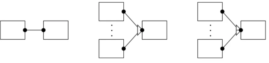
(a) uni-uni (b) uni-and (c) uni-or
Fig. 1.Legal attachments
The architectural topology is specified through the declaration of a set of architectural element instances (AEIs) representing the system components, a set of architectural (as opposed to local) interactions given by some interac-tions of the AEIs that act as interfaces for the whole architectural type, and a set of directed architectural attachments among the interactions of the AEIs. Alternatively, the architectural topology can be specified through the Æmilia graphical notation inspired by flow graphs [38], in which the boxes denote the AEIs, the black circles denote the local interactions, the white squares denote the architectural interactions, and the directed edges denote the attachments.
Every interaction is declared to be an input interaction or an output interac-tion and every attachment must go from an output interacinterac-tion to an input inter-action of two different AEIs. In addition, every interinter-action is declared to be a uni-interaction, an and-uni-interaction, or an or-interaction. As shown in Fig. 1, the only legal attachments are those between two uni-interactions, an and-interaction and a uni-interaction, and an or-interaction and a uni-interaction. An and-interaction and an or-interaction can be attached to several uni-interactions. In the case of execution of an and-interaction, it synchronizes with all the uni-interactions attached to it. In the case of execution of an or-interaction, instead, it synchro-nizes with only one of the uni-interactions attached to it. An AEI can have different types of interactions (input/output, uni/and/or, local/architectural). Every local interaction must be involved in at least one attachment, while every architectural interaction must not be involved in any attachment. No isolated groups of AEIs are admitted in the architectural topology. On the performance side, we have two additional requirements. For the sake of modeling consistency, all the occurrences of an action type in the behavior of an AET must have the
same kind of rate (exponential, or infinite with the same priority level, or passive with the same priority level). In order to comply with the generative-reactive synchronization discipline of EMPAgr, which establishes that two nonpassive ac-tions cannot synchronize, every set of attached interacac-tions must contain at most one interaction whose associated rate is exponential or infinite.
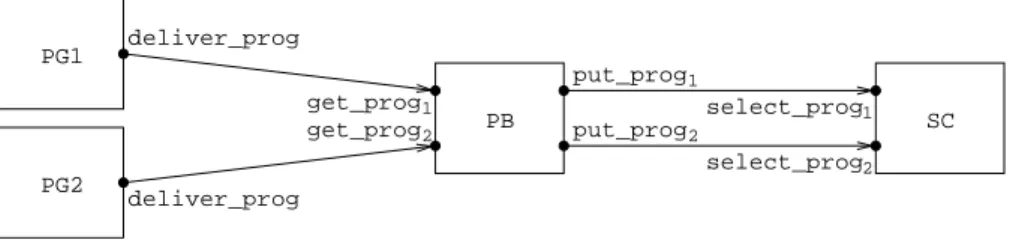
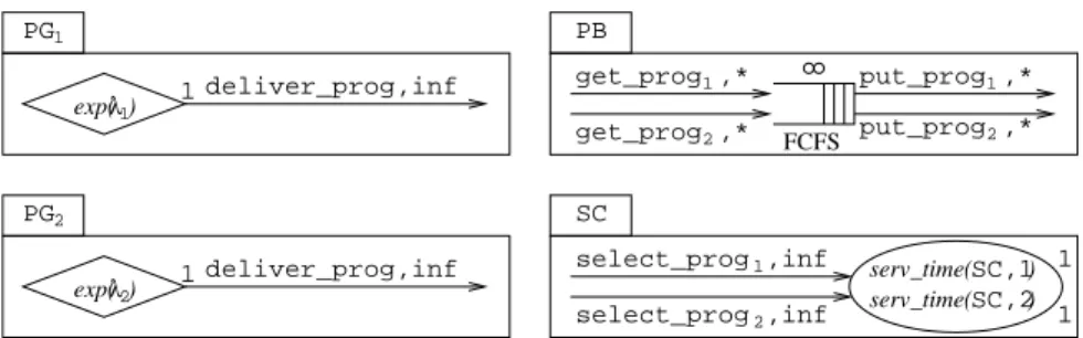
get_prog2 1 get_prog put_prog2 put_prog1 PG1 PG2 PB deliver_prog deliver_prog SC select_prog select_prog1 2
Fig. 2.Graphical description ofSeqCompSys
As an example, we show in Table 2 an Æmilia textual description for an architectural type representing a compiler system. The compiler we consider is a sequential monolithic compiler that carries out all the phases (lexical analy-sis, parsing, type checking, code optimization, and code generation), with each phase introducing an exponentially distributed delay. For the sake of perfor-mance evaluation, the description of the compiler system comprises a generator of programs to be compiled, where the program interarrival times are assumed to follow an exponential distribution, as well as un unbounded buffer in which such programs wait before being compiled one at a time. We suppose that there are two different classes of programs: those whose code must be optimized and those whose code must not. As can be noted, the description of the architectural
type SeqCompSys is parametrized with respect to the arrival rates of the two
classes of programs (λ1, λ2) and the service rates of the five compilation phases
(µl, µp, µc, µo, µg). The omitted values for the priority levels and the weights of
the infinite and passive rates in the specification are taken to be 1. The same sequential compiler system is depicted in Fig. 2 through the Æmilia graphical notation.
2.2 Formal Semantics and Analysis Support
The semantics of an Æmilia specification is given by translation into EMPAgr. This translation is carried out in two steps. In the first step, the semantics of each AEI is defined to be the behavior of the corresponding AET — in which the formal rates, priority levels, and weights are replaced by the corresponding actual ones — projected onto its interactions. Such a projected behavior is ob-tained from the list of sequential EMPAgr defining equations representing the behavior of the AET by applying a hiding operator on all the actions that are not interactions. In this way, we abstract from all the internal details of the
ARCHI TYPE SeqCompSys(rateλ1, λ2, µl, µp, µc, µo, µg)
ARCHI ELEM TYPES
ELEM TYPE ProgGenT(rateλ)
BEHAVIOR ProgGen(void;void) =
<generate prog, λ>.<deliver prog,inf>.ProgGen()
INPUT INTERACTIONS
OUTPUT INTERACTIONS UNI deliver prog
ELEM TYPE ProgBufferT(integer h1,h2) BEHAVIOR ProgBuffer(integer h1,h2;void) =
choice
{
<get prog1,∗>.ProgBuffer(h1+1,h2), <get prog2,∗>.ProgBuffer(h1,h2+1),
cond(h1>0)−> <put prog1,∗>.ProgBuffer(h1−1,h2), cond(h2>0)−> <put prog2,∗>.ProgBuffer(h1,h2−1)
}
INPUT INTERACTIONS UNI get prog1;get prog2 OUTPUT INTERACTIONS UNI put prog1;put prog2 ELEM TYPE SeqCompT(rateµl, µp, µc, µo, µg)
BEHAVIOR SeqComp(void;void) =
choice
{
<select prog1,inf>.<recognize tokens, µl>. <parse phrases, µp>.<check phrases, µc>.
<optimize code, µo>.<generate code, µg>.SeqComp(), <select prog2,inf>.<recognize tokens, µl>.
<parse phrases, µp>.<check phrases, µc>. <generate code, µg>.SeqComp()
}
INPUT INTERACTIONS UNI select prog1;select prog2 OUTPUT INTERACTIONS
ARCHI TOPOLOGY
ARCHI ELEM INSTANCES PG1:ProgGenT(λ1); PG2:ProgGenT(λ2); PB:ProgBufferT(0,0);
SC:SeqCompT(µl, µp, µc, µo, µg)
ARCHI INTERACTIONS
ARCHI ATTACHMENTS FROM PG1.deliver prog TO PB.get prog1; FROM PG2.deliver prog TO PB.get prog2; FROM PB.put prog1TO SC.select prog1; FROM PB.put prog2TO SC.select prog2 END
behavior of the AEI. In addition, the projected behavior must reflect the fact that an or-interaction can result in several distinct synchronizations. Therefore, every or-interaction is rewritten as a choice among as many indexed instances of uni-interactions as there are attachments involving the or-interaction. Recalled that in EMPAgrthe hiding operator is denoted by the symbol ”/”, for our com-piler system example we have:
[[PG1]] =ProgGen1/{generate prog}
[[PG2]] =ProgGen2/{generate prog}
[[PB]] =ProgBuffer(0,0)
[[SC]] =SeqComp/{recognize tokens,parse phrases,check phrases,
optimize code,generate code}
where ProgGen1 (resp.ProgGen2) is obtained fromProgGen by replacing each
occurrence of λwithλ1(resp.λ2).
In the second step, the semantics of an architectural type is obtained by composing in parallel the semantics of its AEIs according to the specified at-tachments, after relabeling to the same fresh action type all the interactions attached to each other. This relabeling is required by the synchronization mech-anism of EMPAgr, which establishes that only actions with the same type can synchronize. Recalled that in EMPAgrthe relabeling operator is denoted by the symbols ”[” and ”]” and that the left-associative parallel composition operator is denoted by the symbol ”kS” where Sis the set of action types on which the
synchronization is enforced, for our compiler system example we have: [[SeqCompSys]] = [[PG1]][deliver prog7→a1] k∅
[[PG2]][deliver prog7→a2] k{a1,a2}
[[PB]][get program17→a1,get program27→a2,
put program17→b1,put program27→b2] k{b1,b2}
[[SC]][select prog17→b1,select prog27→b2]
Given the translation above, Æmilia inherits the semantic models of EMPAgr. More precisely, the semantics of an Æmilia specification is a state-transition graph called the integrated semantic model, whose states are represented by EMPAgrterms and whose transitions are labeled with EMPAgractions together with the related guards arising from the use of thechoiceoperator. This graph is finite state and finitely branching unless variables taking values from infinite domains are used (like in the buffer of the compiler system example), in which case a symbolic representation of the state space is employed in accordance with [13]. After pruning the lower priority transitions from the integrated se-mantic model, it is possible to derive a functional sese-mantic model, by removing the action rates from the transitions, and a performance semantic model, by re-moving the action types from the transitions. The performance semantic model, which is defined only if the integrated semantic model has neither passive tran-sitions nor trantran-sitions with a guard different fromtrue, is a continuous-time or a discrete-time Markov chain [48] depending on whether the integrated semantic model has exponentially timed transitions or not.
On the analysis side, Æmilia inherits from EMPAgr standard techniques to assess functional properties as well as performance measures. Among such tech-niques we mention model checking [23], equivalence checking [24], Markovian
analysis [48] based on rewards [32] as described in [14], and discrete event simu-lation [51], all of which are available in the Æmilia-based software tool TwoTow-ers 3.0 [12]. In addition to these capabilities, Æmilia comes equipped with some specific checks for the detection of architectural mismatches — and the provi-sion of related diagnostic information — that may arise when assembling the components together. The first group of checks ensures that deadlock freedom is preserved when building a system from deadlock-free components [15, 2]. The second group of checks makes sure that assembling components with partially specified performance details (i.e., with passive actions occurring in their behav-iors) results in a system with fully specified performance aspects [16]. Finally, the third group of checks comes into play in case of hierarchical modeling, i.e. whenever the description of a component behavior contains an architectural type invocation. Such checks guarantee that the actual parameters of an invocation of an architectural type conform to the formal parameters of the definition of the architectural type, in the sense that the actual components have the same observable behavior as the corresponding formal components [15] and that the actual topology is a legal extension of the formal topology [17, 18].
3
Queueing Networks
QN models have been widely applied as system performance models to repre-sent and analyze resource sharing systems [34, 35, 37, 33, 42, 50, 8]. In essence, a QN model is a collection of interacting service centers, representing system resources, and a set of customers, representing the users sharing the resources. The customers’ competition for the resource service corresponds to queueing into the service centers. The popularity of QN models for system performance evaluation is due to their relatively high accuracy in performance results and their efficiency in model analysis and evaluation. In this section we briefly recall the basic notions and properties of QN models. In particular, we shall focus on the class of product form QNs, which admit fast solution techniques.
3.1 Queueing Systems
As depicted in Fig. 3(a), the simplest case of QN is the one in which there is a single service center together with a source of arrivals, which is referred to as a queueing system (QS). Every QS is completely described by the customer interarrival time distribution, the customer service time distribution, the number of independent servers, the queue capacity, the customer population size, and the queueing discipline. The first five parameters are summarized by using the Kendall’s notation A/B/m/c/p, with A and B ranging over a set of probability distributions — ’M’ for memoryless distributions, ’D’ for deterministic values, ’PH’ for phase-type distributions, and ’G’ for general distributions — andm,c, and p being natural numbers. If c and p are unspecified, they are assumed to be∞, i.e. to describe an unlimited queue capacity and an unlimited population.
Every customer needing a certain service arrives at the QS, waits in the queue for a while, is served by one of the servers, and finally leaves the QS.
The queueing discipline is an algorithm that determines the order in which the customers in the queue are served. Such a scheduling algorithm may depend on the order in which the customers arrive at the QS, the priorities assigned to the customers, or the amounts of service already provided to the customers. Here are some commonly adopted queueing disciplines:
– First come first served (FCFS): the customers are served in the order of their arrival.
– Last come first served (LCFS): the customers are served in the reverse order of their arrival.
– Service in random order (SIRO): the next customer to be served is chosen probabilistically, with equal probabilities assigned to all the waiting cus-tomers.
– Nonpreemptive priority (NP): the customers are assigned fixed priorities; the waiting customer with the highest priority is served first; if several waiting customers have the same highest priority, they are served in the order of their arrival; once begun, a service cannot be interrupted by the arrival of a higher priority customer.
– Preemptive priority (PP): same as NP, but each arriving higher priority customer interrupts the current service, if any, and begins to be served; a customer whose service was interrupted resumes service at the point of interruption when there are no higher priority customers to be served. – Last come first served preemptive resume (LCFS-PR): same as LCFS, but
each arriving customer interrupts the current service, if any, and begins to be served; the interrupted service of a customer is resumed when all the customers that arrived later than that customer have departed.
– Round robin (RR): each customer is given continuous service for a maximum interval of time called a quantum; if the customer’s service demand is not satisfied during the quantum, the customer reenters the queue and waits to receive an additional quantum, repeating this process until its service demand is satisfied; the waiting customers are served in the order in which they last entered the queue.
– Processor sharing (PS): all the waiting customers receive service simultane-ously with equal shares of the service rate.
– Infinite server (IS): no queueing takes place as each arriving customer always find an available server.
If the queueing discipline is omitted in the QS notation, it is assumed to be FCFS.
The QS behavior can be analyzed either during a given time interval (tran-sient analysis) or by assuming that it reaches a stationary condition (steady-state analysis). The analysis of the QS is based on the definition of an underlying continuous-time Markov chain. The QS steady-state analysis usually evaluates a set of four average performance indices after computing the queue length dis-tribution, i.e. the distribution of the number of customers in the QS. The four
queue server
arrivals departures
(a) A QS (b) A simple closed QN
Fig. 3.QN graphical representation
average performance indices are the throughput (mean number of customers leaving the system per unit of time), the utilization (average fraction of time during which the servers are used), the mean number of customers in the QS, and the mean response time experienced by the customers visiting the QS.
For instance, let us consider the simplest case of QS M/M/1 with arrival rate λand service rate µ [34]. Although the stochastic process underlying the QS M/M/1 is an infinite-state continuous-time Markov chain, where each state represents the number of customers in the system, the particular structure of this Markov chain allows us to easily derive that the distribution of the numberN1of customers in the system — on the basis of which the four average measures above are defined — is geometrical with parameter given by the traffic intensityρ1=
λ/µ. The steady-state analysis of this QS requires that the stability condition
ρ1<1 holds, i.e., that the customer arrival rate is less than the service rate. In this case we can easily derive the four average perfomance indices as follows:
– The throughput is given by the probability that there is at least one customer in the system multiplied by the service rate, i.e.X1 = Pr{N1 > 0} ·µ =
ρ1·µ=λ.
– The utilization is given by the probability that there is at least one customer in the system, i.e.U1= Pr{N1>0}=ρ1.
– The mean number of customers in the system is the expected value of the geometrical distribution describing the number of customers in the system, i.e.N1=ρ1/(1−ρ1).
– The mean response time is obtained from Little’s law as the ratio of the mean number of customers in the system to the arrival rate, i.e. R1 = N1/λ = 1/[µ·(1−ρ1)].
It can be shown that all the queueing disciplines with noninterruptable, nonpri-oritized service — like FCFS, LCFS, and SIRO — together with PS — which is a good approximation of RR — and LCFS-PR are equivalent with respect to the four average performance measures above for a QS M/M/1.
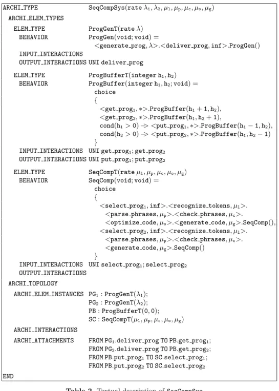
In the more general case of a QS M/M/mwith arrival rate λ, which has m
identical servers that operate independently and in parallel each with service rateµ, the traffic intensity is defined byρm=λ/(m·µ) and, under the stability
Xm= mP−1 i=1 i·µ·Pr{Nm=i}+ ∞ P i=m m·µ·Pr{Nm=i}=λ Um= 1−Pr{Nm= 0} Nm=m·ρm+Pr{Nm=0}·ρm·(m·ρm) m m!·(1−ρm)2 Rm= 1µ· ³ 1 +Pr{Nm=0}·ρm·(m·ρm)m−1 m!·(1−ρm)2 ´ where: Pr{Nm= 0}= Ãm−1 X i=0 (m·ρm)i i! + (m·ρm)m m!·(1−ρm) !−1
3.2 Networks of Queueing Systems
A QN is composed of a set of interconnected service centers. When describing a QN, which can be represented — as shown in Fig. 3(b) — through a directed graph whose nodes are the service centers and whose edges represent the behavior of the customers’ service requests, it is necessary to specify for each service center the service time distribution, the number of servers, the queue capacity, the queueing discipline, and the routing probabilities for the customers leaving the service center. A QN can be open or closed, depending on whether external arrivals and departures are allowed or not, or mixed. In an open QN, a customer that completes service at a service center immediately enters another service center, reenters the same service center, or departs from the network. In a closed QN, instead, a fixed number of customers circulate indefinitely among the service centers. 1 s 2 s s3 f class class e class class class b a c d class closed chain open chain
Fig. 4.A mixed network with three service centers, an open chain with classesa, b, e,
and a closed chain with classesc, d, f.
Different types of customers in the QN model can be used to represent dif-ferent behaviors. This in fact allows various types of external arrival process, different service demands, and different types of network routing to be modeled. A chain gathers the customers of the same type. A chain consists then of a set of classes that represent different phases of processing in the system for a given type of customers. Classes are partitioned within the service centers and each customer in a chain moves between the classes. A chain can be used to represent
a customer routing behavior dependent on the past history. For example, two classes of the same chain in a service center can represent the customer require-ment of two successive services. Each chain can be open or closed depending on whether external arrivals and departures are allowed or not. Multiclass or multichain networks can be open or closed if all the chains are open or closed, respectively. A mixed network has both open and closed chains. Fig. 4 shows an example of a multiclass network with two chains and six classes. The open chain describes the routing behavior of the type 1 customers: two successive visits to the service center s1 followed by a visit to service center s3. Chain 2 is closed and there is a constant number of type 2 customers circulating between service centers s1,s2, ands3.
Evaluating a QN model means obtaining a quantitative description of its behavior by computing a set of figures of merit, such as the four average perfor-mance indices considered for a single QS. The analysis of a QN model provides information both on the local and on the global performance, i.e. the performance of each service center and the overall system performance. A QN can be analyzed by defining and solving the underlying stochastic process, which under general assumptions is a countinous-time Markov chain. Unfortunately, its solution can often become unfeasible since its state space size grows exponentially with the number of components of the QN model. However, some efficient solution algo-rithms can be defined for the special subclass of product form QNs, which we briefly introduce in the next section. Such algorithms provide a powerful tool for performance analysis based on QNs.
3.3 Product Form QNs
Product form QNs (see [6] for a complete survey) avoids the state space explosion problem because they can be solved compositionally. Given that the state of a QN is a tuple consisting of the number of customers in the various service centers, the probability of a product form QN state is simply obtained as the product of the probabilities of its constituent service center states, up to a normalizing constant in the case of closed QNs. An important characterization of product form QNs is given by the BCMP theorem [10], which defines the BCMP class of product form open, closed and mixed QNs with multiple classes of customers, Poisson arrivals (i.e. exponentially distributed interarrival times) with rates possibly depending on the total population of the QN or on the population of a chain, and arbitrary Markovian routing. According to the BCMP theorem, each multiclass service center can have one combination of the following queueing disciplines and service time distributions:
– FCFS with exponentially distributed service times, with the same rate for all the classes of customers;
– PS, LCFS-PR, or IS with phase-type distributed service times, possibly dif-ferent for the various classes of customers.
In the second case, only the expected values of the phase-type service time distributions affect the QN solution in terms of the four average performance
indices, so when computing such indices the phase-type distributions can be replaced with exponential distributions having the same expected values.
In the case of an open product form QN, the four average performance mea-sures can easily be obtained at the global level and at the local level from the analysis of the constituent service centers, when considered as isolated QSs with Poisson arrivals, by exploiting the two groups of formulas at the end of Sect. 3.1. The arrival rates are derived by solving the linear system of the traffic equa-tions defined by the routing probabilities among the service centers. The same average indices can be obtained at the global level and at the local level for a closed or mixed product form QN by applying one of the following algorithms: the convolution algorithm [19], the mean-value analysis algorithm (MVA) [44], the local balance algorithm for normalizing constants (LBANC) [20], and the recursion-by-chain algorithm (RECAL) [25]. These algorithms also provide the basis for most approximate analytical methods that need to be applied whenever the QN model under consideration does not belong to the class of product form QNs (see, e.g., [36]).
An important property of product form QNs is exact aggregation, which al-lows replacing a subnetwork with a single service center, in such a way that the new aggregated QN has the same behavior in terms of the four average perfor-mance indices. Thus, exact aggregation can be used to represent and evaluate a system at different levels of abstraction. Moreover, exact aggregation for prod-uct form QNs provides a basis for approximate solution methods of more general QNs that are not product form (see, e.g., [36]).
Various extensions of the class of BCMP product form QNs have been de-rived. They include QNs with other queueing disciplines, QNs with state depen-dent routing, some special cases of QNs with finite capacity queues, subnetwork popolation constraints, and blocking, and QNs with batch arrivals and batch services. Another extension of QNs networks with product form is the class of G-networks [28], which comprise both positive and negative customers.
3.4 QN Extensions
Extensions of classical QN models, named extended QN (EQN) models, have been introduced in order to represent several interesting features of real systems, such as synchronization and concurrency constraints, finite capacity queues, memory constraints, and simultaneous resource possession.
In particular, concurrency and synchronization among tasks are represented in an EQN model by fork and join nodes. A fork node starts the parallel execution on distinct service centers of the different tasks in which a customer’s request can be split, while a join node represents a synchronization point for the termination of all such tasks. A few cases of QNs with forks and joins have been solved with exact and approximate analytical techniques (see, e.g., [40, 4, 9]).
QNs with finite capacity queues and blocking have been introduced as more realistic models of systems with finite resources and population constraints. When a customer arrives at a finite capacity queue that is full, the customer cannot enter the queue and it is blocked. Various blocking mechanisms can be
defined — like blocking after or before service and repetitive service — that specify the behavior of the customers blocked in the network. Except for a few cases that admit product form solutions, QNs with blocking are solved through approximate techniques (see, e.g., [42, 8]).
Another extension of the QN model is given by the layered queueing network (LQN) model, which allows client-server communication patterns to be modeled in concurrent and/or distributed software systems. LQN models can be solved by analytic approximation methods based on standard methods for EQNs with simultaneous resource possession and MVA (see, e.g., [45, 52, 27]).
The exact and approximate analytical methods for solving EQNs require that a set of assumptions and constraints are satisfied. Should this not be the case, EQN models can be analyzed via simulation, at the cost of higher development and computational times to obtain accurate results.
Examples of performance evaluation tools based on QNs and their extensions are RESQ [21], QNAP2 [49], HIT [11], and LQNS [26].
4
Translating Æmilia Specifications into QN Models
In this section we provide a translation that maps an Æmilia specification into a QN model to be used to predict and improve the performance of the described SA. As mentioned in Sect. 1, there are several good reasons for resorting to QN models at the SA level of design, instead of the flat state-transition graphs used as semantic models for Æmilia. First, QNs are structured performance models whose constituent service centers can be put in correspondence with groups of AEIs of the Æmilia specifications. Second, typical average performance measures can be computed at the level of the overall QNs and interpreted at the level of the groups of AEIs of the Æmilia specifications corresponding to their constituent service centers, thus providing a useful feedback. Third, QNs do not suffer from the state space explosion problem, as they are equipped with efficient solution techniques that avoid the construction of the state space. Finally, QNs can sometimes be solved symbolically, without having to instantiate the values of the corresponding parameters in the Æmilia specifications.
To carry out the translation, first of all we observe that the two formalisms that we are considering are quite different from each other. On the one hand, Æmilia is a component-oriented language for handling both functional and per-formance characteristics, in which all the details must be expressed in an action-based way. On the other hand, QNs result in a queue-oriented graphical notation for performance modeling purposes only, in which some details — notably the queueing disciplines — are described in natural language. As a consequence, there will be Æmilia specifications that cannot be converted into QN models, either because they do not follow a queue-oriented pattern, or because it is hard to understand — by looking at their process algebraic defining equations — the queueing disciplines that they encode. Therefore, we shall impose some general syntax restrictions that single out a reasonably wide class of Æmilia specifica-tions for which a QN model may be derived.
Within the class of Æmilia specifications that obey the general syntax re-strictions, given a specification we try to map each of its constituent AEIs into a part of a QN model. In principle, it would seem to be natural to map each AEI into a QS PH/PH/m/c/p. However, this is not always possible because the AEIs are usually finer than the QSs. As a consequence, we identify five classes of QN basic elements — which we call arrival processes, buffers, fork processes, join processes, and service processes, respectively, and graphically represent through an extension of the traditional notation used for QNs — and we impose some further specific syntax restrictions to single out those AEIs that fall into one of the five classes. For each Æmilia specification obeying both the general and the specific syntax restrictions, the translation is accomplished by first mapping each of its constituent AEIs into the corresponding QN basic element and then composing the previously obtained QN basic elements according to the attach-ments declared in the Æmilia specification. The translation will be illustrated by means of the sequential compiler system example introduced in Sect. 2. 4.1 General Syntax Restrictions: Benefits and Limitations
The general syntax restrictions helps identifying the Æmilia specifications for which it is possible to derive an open, closed or mixed QN model comprising ar-rival processes, buffers, fork processes, join processes, and service processes. The general restrictions are mainly based on the observation that an AEI describes a sequential software component, which thus runs on a single computational resource.
The first general restriction is that every AEI of an Æmilia specification must be an arrival process, a buffer, a fork process, a join process, or a service process, and must be properly connected to the other AEIs in order to obtain a well-formed QN. This is achieved through specific syntax restrictions depending on the particular QN basic element, which will be introduced in the next sections. The second general restriction aims at easing the identification of those AETs that represent arrival or service processes, which are built around exponentially timed actions describing the relevant delays. The second general restriction es-tablishes that the interactions of an Æmilia specification cannot be exponentially timed, i.e. they must be immediate or passive.
The third general restriction aims at avoiding the unnatural application of the race policy to several distinct activities within the same (sequential) AEI, thus causing the various arrival and service processes to be modeled separately with different AEIs. The third general restriction establishes that, within the behavior of the AETs of an Æmilia specification, no exponentially timed action can be alternative to another exponentially timed action.
The fourth general restriction aims at allowing interarrival and service times to be characterized through precisely defined phase-type distributions. The fourth general restriction establishes that, within the behavior of the AETs of an Æmilia specification, no exponentially timed action can be alternative to an immediate or passive action, no immediate action can be alternative to a passive action, and no interaction can be alternative to a local action.
The last three general restrictions, as well as the specific restrictions illus-trated in the next sections that implement the first general restriction, can au-tomatically be checked at the syntax level, without constructing the underlying state space of the entire Æmilia specification. They preserve much of the mod-eling power that Æmilia inherits from EMPAgr, without hampering the descrip-tion of typical situadescrip-tions like parallel execudescrip-tions, synchronizadescrip-tion constraints, probabilistic/prioritized choices, and activities whose duration is or can be ap-proximated with a phase-type distribution. It is straightforward to verify that SeqCompSys defined in Table 2 satisfies the last three general restrictions.
The four general restrictions, together with the specific syntax restrictions accompanying the first general one, introduce two main limitations. First, due to the fourth general restriction, the Æmilia specifications modeling preemption cannot be dealt with, as it is not possible to express the fact that the service of a customer of a certain class is interrupted by the arrival of a customer of another class having higher service priority. Second, as we shall see when presenting the specific syntax restrictions for the buffers, we only address queueing disciplines with noninterruptable service for a fixed number of servers, like FCFS, LCFS, SIRO, and NP, thus excluding those policies in which the service of a customer can be interrupted (PP, LCFS-PR) or divided into several rounds (RR, PS), as well as those policies in which no queueing takes place as every incoming customer always finds an available server (IS).
4.2 Modeling Phase-Type Distributions
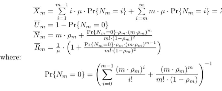
Since the interarrival times and the service times are allowed to follow phase-type distributions, before proceeding with the translation it is worth recalling how the phase-type distributions can be modeled in a language like Æmilia, where only exponentially distributed delays can directly be specified. A continu-ous phase-type distribution [41] describes the time to absorption in a finite-state continuous-time Markov chain having exactly one absorbing state. Well known examples of phase-type distributions are the exponential distribution, the hypo-exponential distribution, the hyperhypo-exponential distribution, and combinations thereof, which are characterized in terms of time to absorption in a finite-state continuous-time Markov chain with one absorbing state as depicted in Fig. 5, where the numbers labeling the states describe the initial state probability func-tions.
Observed that an absorbing state can be modeled by term stop, the three phase-type distributions above can easily be modeled through a suitable inter-play of exponentially timed actions and immediate actions as follows. An expo-nential distribution with rateλcan be modeled through the following equation:
Expλ(void;void) =<phase, λ>.stop
Ann-stage hypoexponential distribution with rates λ1, . . . , λn can be modeled
through the following equation:
Hypoexpλ1,...,λm(void;void) =<phase, λ1>. . . . .<phase, λn>.stop
λ 1
(a) Exponential distribution
λ2 p1 λ1 λn p2 pn (c) Hyperexponential distribution ... λ2 λ1 λn 1 (b) Hypoexponential distribution ...
Fig. 5.Typical phase-type distributions
probabilitiesp1, . . . ,pncan be modeled through the following equation: Hyperexpλ1,...,λn,p1,...,pn(void;void) =
choice {
<branch,inf(1,p1)>.<phase, λ1>.stop,
.. .
<branch,inf(1,pn)>.<phase, λn>.stop }
In the arrival processes and in the service processes with phase-type dis-tributed delays, the occurrences ofstopwill be replaced by suitable invocations of the behaviors that must take place after the delays have elapsed.
4.3 Arrival Processes
An arrival process is a generator of arrivals of customers of a certain class, whose interarrival times follow a phase-type distribution. As depicted in Fig. 6, we distinguish between two different kinds of arrival processes depending on whether the related customer population is unbounded or finite.
1 deliver ,inf n deliver ,inf 1 n rp rp 1 n rp rp
(a) Arrival process for unbounded population (b) Arrival process for single customer of finite population
return ,*1 return ,*m n deliver ,inf 1 deliver ,inf int_arr_time int_arr_time
Fig. 6.Graphical representation of the arrival processes
In the case of an unbounded customer population, the customer interarrival time distribution refers to the whole population, so there is no need to explicitly model the return of a customer after its service termination. As an example, the behavior of an AEI, which acts as an arrival process for an unbounded pop-ulation of customers whose interarrival time is exponentially distributed with
rate λ, where each customer has a set of n different forks or service centers as destinations chosen according to the intraclass routing probabilitiesrp1, . . . ,rpn,
must be equivalent3 to the following one:
UnboundedPopArrProc(void;void) =
<generate, λ>.UnboundedPopArrProc0() UnboundedPopArrProc0(void;void) =
choice {
<choose1,inf(1,rp1)>.<deliver1,inf>.UnboundedPopArrProc(),
.. .
<choosen,inf(1,rpn)>.<delivern,inf>.UnboundedPopArrProc() }
withdeliver1, . . . ,delivern being output interactions attached to input
inter-actions of buffers (not related to join processes), fork processes with no buffer, or service processes with no buffer. The specific syntax restriction requires that, in order for an AEI to be classified as an arrival process for an unbounded popu-lation of customers, its behavior and interactions must be equivalent to the pre-vious ones, with: the exponentially timed action possibly replaced by a term de-scribing a more general phase-type distribution whereUnboundedPopArrProc’() is substituted for each occurrence ofstop; the destination choice actions omit-ted if there is only one possible destination; the delivery actions possibly having specific priority levels and specific weights if the related destinations are service processes with no buffer.
If the customer population is finite, instead, then the customer interarrival time distribution for the whole population varies proportionally to the number of customers that are not requesting any service, hence the return of a customer after its service termination must explicitly be modeled. In this case, the cus-tomers are represented separately through independent instances of the same AET with the same individual interarrival time distribution, in order to easily achieve the global interarrival time distribution scaling. For instance, the behav-ior of an AEI, which acts as an arrival process for a single customer belonging to a finite population of customers whose individual interarrival time is exponen-tially distributed with rateλ, where the customer has a set ofndifferent forks or service centers as destinations chosen according to the intraclass routing prob-abilities rp1, . . . ,rpn and can return from m distinct joins or service processes,
must be equivalent to the following one:
3 In our framework, equivalence can formally be checked on the basis of the notion of strong extended Markovian bisimulation [14].
SingleCustArrProc(void;void) =
<generate, λ>.SingleCustArrProc0() SingleCustArrProc0(void;void) =
choice {
<choose1,inf(1,rp1)>.<deliver1,inf>.SingleCustArrProc00(),
.. .
<choosen,inf(1,rpn)>.<delivern,inf>.SingleCustArrProc00() }
SingleCustArrProc00(void;void) = choice { <return1,∗>.SingleCustArrProc(), .. . <returnm,∗>.SingleCustArrProc() }
with: deliver1, . . . ,delivern being output interactions attached to input
or-interactions of buffers (not related to join processes), fork processes with no buffer, or service processes with no buffer; return1, . . . ,returnm being input
interactions attached to output or-interactions of join processes or service pro-cesses. The specific syntax restriction requires that, in order for an AEI to be classified as an arrival process for a single customer belonging to a finite pop-ulation of customers, its behavior and interactions must be equivalent to the previous ones, with the remaining constraints similar to those for the arrival processes for unbounded populations. In addition, all the AEIs modeling the customers of the same finite population must be instances of the same AET characterized by the same individual interarrival time distribution and must be attached to the same input or-interactions of buffers (not related to join pro-cesses), fork processes with no buffer, or service processes with no buffer as well as to the same output or-interactions of join processes or service processes.
To conclude, for the sequential compiler system of Sect. 2 we observe that PG1andPG2are arrival processes for unbounded populations of customers of two
different classes, each having a single destination. 4.4 Buffers
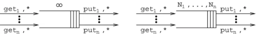
A buffer is a repository of customers of different classes that are waiting to be served. As depicted in Fig. 7, we distinguish between two different kinds of buffers depending on their capacity.
In the case of an unbounded buffer, the incoming customers can always be accommodated within the buffer. The specific syntax restriction requires that, in order for an AEI to be classified as an unbounded buffer for nclasses of cus-tomers, it must have a behavior equivalent to the following one:
(a) Unbounded buffer
1
(b) Finite capacity buffer
get ,* get ,*n 1 put ,*1 put ,*n get ,*1 get ,*n put ,* put ,* 1 n N ,...,Nn
Fig. 7.Graphical representation of the buffers
UnboundedBuffer(integer h1, . . . ,hn;void) = choice { <get1,∗>.UnboundedBuffer(h1+1, . . . ,hn), .. . <getn,∗>.UnboundedBuffer(h1, . . . ,hn+1),
cond(h1>0)−> <put1,∗>.UnboundedBuffer(h1−1, . . . ,hn),
.. .
cond(hn>0)−> <putn,∗>.UnboundedBuffer(h1, . . . ,hn−1) }
with: h1, . . . ,hninitially set to nonnegative integers;get1, . . . ,getn being input
interactions attached to output interactions of arrival processes, fork processes, join processes, or service processes;put1, . . . ,putnbeing output interactions
at-tached to input interactions of fork processes with buffer, join processes with buffers, or service processes with buffer; geti being an input or-interaction if
the customers of class i belong to a finite population and come directly from their arrival processes.
If the buffer capacity is finite, instead, then the incoming customers can be accommodated only if the buffer capacity is not exceeded. The specific syntax restriction requires that, in order for an AEI to be classified as a finite capacity buffer fornclasses of customers, where the customers of classican occupy up to Nipositions in the buffer, it must have a behavior equivalent to the following one:
FiniteCapBuffer(integer(0..N1)h1, . . . ,integer(0..Nn)hn;void) = choice
{
cond(h1<N1)−> <get1,∗>.FiniteCapBuffer(h1+1, . . . ,hn),
.. .
cond(hn<Nn)−> <getn,∗>.FiniteCapBuffer(h1, . . . ,hn+1), cond(h1>0)−> <put1,∗>.FiniteCapBuffer(h1−1, . . . ,hn),
.. .
cond(hn>0)−> <putn,∗>.FiniteCapBuffer(h1, . . . ,hn−1) }
with the remaining constraints equal to those for the unbounded buffers, except for the fact that now the initial values of h1, . . . ,hn cannot exceed the
It is worth observing that the buffers outlined above do not make any as-sumption about the order in which the customers of the same class are taken from the buffer with respect to the order in which they arrive at the buffer. Therefore, from the point of view of the four average performance indices intro-duced in Sect. 3.1, such buffers can be used to support any queueing discipline with noninterruptable service, like FCFS, LCFS, SIRO, and NP. On the con-trary, the buffers above cannot be used to describe those queueing disciplines in which the service of a customer can be interrupted (PP, LCFS-PR), or can be divided into several rounds (RR, PS), or can immediately take place (IS).
To conclude, for the sequential compiler system of Sect. 2 we observe that PBis an unbounded buffer for two classes of customers.
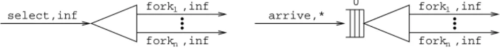
4.5 Fork Processes
A fork process handles the splitting of each request of the customers of a certain class into several subrequests to be served in parallel by different service centers. As depicted in Fig. 8, we distinguish between two different kinds of fork processes depending on the presence or the absence of a buffer — modeled by another AEI — where the customers can wait before being split.
0
select,inf arrive,*
(a) Fork process with buffer (b) Fork process with no buffer
fork ,inf
fork ,infn
1 fork ,inf1
fork ,infn
Fig. 8.Graphical representation of the fork processes
In the case of a fork process equipped with a buffer, the description of the fork process starts with the selection of the next customer to be split from the buffer. The specific syntax restriction requires that, in order for an AEI to be classified as a fork process equipped with a buffer, where the subrequests are forwarded tondifferent forks or service centers, it must have a behavior equiv-alent to the following one:
ForkProcWithBuffer(void;void) =
<select,inf>.<fork1,inf>. . . . .<forkn,inf>.ForkProcWithBuffer()
with:selectbeing an input interaction attached to the output interaction of a buffer;fork1, . . . ,forknbeing output interactions attached to input interactions
of buffers (not related to join processes), fork processes with no buffer, or service processes with no buffer; the fork actions possibly having specific priority levels and specific weights if the related destinations are service processes with no buffer.
In the case of a fork process with no buffer, instead, the description of the fork process starts with the arrival of the next customer to be split directly from
an arrival process, a fork, a join, or a service center. The specific syntax restric-tion requires that, in order for an AEI to be classified as a fork process with no buffer, where the subrequests are forwarded to n different forks or service centers, it must have a behavior equivalent to the following one:
ForkProcNoBuffer(void;void) =
<arrive,∗>.<fork1,inf>. . . . .<forkn,inf>.ForkProcNoBuffer()
with arrive being an input interaction — or an input or-interaction if the
customers belong to a finite population and come directly from their arrival pro-cesses — attached to an output interaction of an arrival process, a fork process, a join process, or a service process and the remaining constraints equal to those for the fork processes equipped with a buffer.
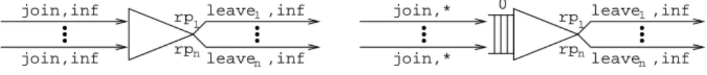
4.6 Join Processes
A join process handles the merging of the subrequests of the customers of a certain class after they have been served in parallel by different service centers. As depicted in Fig. 9, we distinguish between two different kinds of join processes depending on the presence or the absence of buffers — modeled by other AEIs — where the subrequests can wait before being merged.
1 n rp rp leave ,inf1 leave ,infn 1 n rp rp leave ,inf1 leave ,infn 0
(a) Join process with buffers (b) Join process with no buffers
join,inf
join,inf
join,*
join,*
Fig. 9.Graphical representation of the join processes
In the case of a join process equipped with buffers, the description of the join process starts with the selection of the next subrequests to be merged from the buffers. The specific syntax restriction requires that, in order for an AEI to be classified as a join process equipped with buffers, where the subrequests are for-warded by several different joins or service centers and the result of the merging has a set ofndifferent finite population arrival processes, forks, joins, or service centers as destinations chosen according to the intraclass routing probabilities rp1, . . . ,rpn, it must have a behavior equivalent to the following one:
JoinProcWithBuffer(void;void) =
<join,inf>.JoinProcWithBuffer0() JoinProcWithBuffer0(void;void) =
choice {
<choose1,inf(1,rp1)>.<leave1,inf>.JoinProcWithBuffer(),
.. .
<choosen,inf(1,rpn)>.<leaven,inf>.JoinProcWithBuffer() }
with: join being an input and-interaction attached to the output interaction of each buffer; leave1, . . . ,leaven being output interactions attached to input
interactions of arrival processes for finite populations, buffers, fork processes with no buffer, join processes with no buffers, or service processes with no buffer; the destination choice actions omitted if there is only one possible destination; the departure actions possibly having specific priority levels and specific weights if the related destinations are service processes with no buffer; the departure actions omitted if the related destinations are arrival processes for unbounded populations;leaveibeing an output or-interaction if destinationiis an arrival
process for a finite population.
In the case of a join process with no buffers, instead, the description of the join process starts with the arrival of the subrequests to be merged directly from a join or a service center. The specific syntax restriction requires that, in order for an AEI to be classified as a join process with no buffers, with the same char-acteristics as in the previous example, it must have a behavior equivalent to the following one:
JoinProcNoBuffer(void;void) =
<join,∗>.JoinProcNoBuffer0() JoinProcNoBuffer0(void;void) =
choice {
<choose1,inf(1,rp1)>.<leave1,inf>.JoinProcNoBuffer(),
.. .
<choosen,inf(1,rpn)>.<leaven,inf>.JoinProcNoBuffer() }
withjoinbeing an input and-interaction attached to output interactions of join processes or service processes and the remaining constraints equal to those for the join processes equipped with buffers.
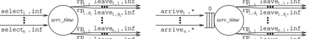
4.7 Service Processes
A service process is a server for customers of different classes, whose service times follow a phase-type distribution. As depicted in Fig. 10, we distinguish between two different kinds of service processes depending on the presence or the absence of a buffer — modeled by another AEI — where the customers can wait before being served.
In the case of a service process equipped with a buffer, the description of the service process starts with the selection of the next customer to be served from the buffer. As an example, the behavior of an AEI, which acts as a service process equipped with a buffer that serves customers ofndifferent classes, where each class ihas priority prioi to be selected, probabilityprobito be selected
among the classes with the same priority, exponentially distributed service time with rate µi, and a set of didifferent finite population arrival processes, forks,
joins, or service centers as destinations chosen according to the intraclass routing probabilities rpi,1, . . . ,rpi,di, respectively, must be equivalent to the following
select ,infn 1 select ,inf leave ,inf leave ,inf n,1 n,1 n,dn rp rp leave ,inf leave ,inf rp rp 1,1 1,1 1,d1 1,d1 n n,d leave ,inf leave ,inf n,1 n,1 n,dn rp rp leave ,inf leave ,inf rp rp 1,1 1,1 1,d1 1,d1 n n,d serv_time 0 serv_time arrive ,*1 arrive ,*n
(a) Service process with buffer (b) Service process with no buffer
Fig. 10.Graphical representation of the service processes
one:
ServProcWithBuffer(void;void) =
choice {
<select1,inf(prio1,prob1)>.ServProcWithBuffer01(),
.. .
<selectn,inf(prion,probn)>.ServProcWithBuffer0n() } ServProcWithBuffer0 i(void;void) = <servei, µi>.ServProcWithBuffer00i() ServProcWithBuffer00 i(void;void) = choice {
<choosei,inf(1,rpi,1)>.<leavei,1,inf>.ServProcWithBuffer(),
.. .
<choosei,inf(1,rpi,di)>.<leavei,di,inf>.ServProcWithBuffer() }
with: select1, . . . ,selectn being input interactions attached to the output
in-teractions of a buffer;leave1,1, . . . ,leaven,dn being output interactions attached
to input interactions of arrival processes for finite populations, buffers, fork pro-cesses with no buffer, join propro-cesses with no buffers, or service propro-cesses with no buffer. The specific syntax restriction requires that, in order for an AEI to be classified as a service process equipped with a buffer, its behavior and inter-actions must be equivalent to the previous ones, with: the exponentially timed actions possibly replaced for certain classes of customers by terms describing more general phase-type distributions whereServProcWithBuffer00
i() is
substi-tuted for each occurrence of stop; the destination choice actions omitted for those classes of customers for which there is only one possible destination; the departure actions possibly having specific priority levels and specific weights if the related destinations are service processes with no buffer; the departure actions omitted if the related destinations are arrival processes for unbounded populations; the departure actions being output or-interactions if the related destinations are arrival processes for finite populations.
In the case of a service process with no buffer, instead, the description of the service process starts with the arrival of the next customer to be served