PRICING
CLIMATE
CHANGE
6.1 IntroductionBurning of fossil fuel is the main reason behind man-made climate change. By burning the carbon content, carbon dioxide is produced and quickly spreads in the global atmosphere. This increases the greenhouse effect, thereby changing the earth’s energy balance. Concern over the negative consequences of climate change has led to a vast array of policy measures aimed at reducing the use of fossil fuel. This chapter examines some aspects of these policies. It discusses the argu-ments for taxes and quantity restrictions on CO2 -emit-ting activities, and especially on the burning of fossil fuel, as well as policies to subsidise substitutes for these activities, particularly the use and development of tech-nologies producing non-fossil based “green energy”.
Before moving on to discuss policy, the next section describes important aspects of the production and use of energy in the European Union.
6.2 Energy production and use in the European Union
Europe is heavily dependent on fossil fuel. Figure 6.1 shows energy consumption in the European Union by primary source. The main
prima-ry sources are:
• fossil fuels, consisting of coal and lignite, oil and gas, • nuclear,
• renewables.
Figure 6.1 shows that over the last twenty years, fossil fuel has represented a fairly stable share of around 80 percent of our total energy consumption. There has only been a modest decline over this period: from 83 percent in 1990 to 77 percent in 2008. Meanwhile total energy con-sumption has increased
moder-ately over this period, by 0.4 percent per year, which is substantially less then GDP growth over the same period. Thus, energy efficiency, measured as GDP per unit of energy use has increased.
While the share of fossil energy has remained stable, there have been some changes in its composition. The share of coal and lignite has fallen from around 33 percent to 20 percent of fossil energy, while gas has increased by nearly the same amount, from 21 percent to 32 percent, leaving oil to account for a stable share of slightly below half of total fossil ener-gy consumption.
Non-fossil energy sources as a share of energy con-sumption have increased somewhat over the period. Nuclear power’s share increased from 12.2 percent in 1990, peaking at 14.5 percent in 2002 and then falling slightly to 13.4 percent. Renewables have almost dou-bled relative to their initial share of 4.4 percent, but remain a minor source of energy accounting for just 8.4 percent of total energy consumption in 2008.
Figure 6.2 shows the components of renewable ener-gy over the same period of time. Biomass and wastes increased over the period from 61 percent to 70 per-cent of total renewable energy. The fastest growth
rate, however, occurred in wind energy, which
increased from practically zero in 1990 to account for
0 10 20 30 40 50 60 70 80 90 100
Energy consumption by source in the EU-27
Source: European Environment Agency, “Total primary energy consumption by energy source in 2008, EU-27”. % Renewables Nuclear Gas Oil
Coal and lignite
Other Figure 6.1
7 percent of renewable energy in 2008. It is worth not-ing, however, that this figure only represents 0.56 per-cent of total energy consumption. Hydro power has remained constant in terms of total energy provision and has thus fallen as a share of renewable energy, from 35 percent to 19 percent over the whole period. Geothermal energy, on the other hand, has grown at the same rate as renewables overall, remaining a con-stant share of around 4 percent. Solar power has experienced high growth, but at the end of the period it still only accounted for 1 percent of the 8.4 percent total for renewables.
Finally, let us break down the biomass and wastes com-ponent. Figure 6.3 shows that wood and wood waste is the largest component, although other wastes, biogas and biofuels have all increased. For example, biofuels and biogas together account for 18 per cent of biomass
and wastes, implying that they represent 1.5 percent of total energy consumption.
Over the period renewable energy has enjoyed substantial growth. It has increased at an average growth rate of 4.2 percent, while overall energy consumption has only grown by 0.4 percent per year. By the laws of mathematics, this means that the share of renewables will continue to grow if these trends continue. Un -fortunately, achieving a substan-tial share will take a long time at this growth rate. By extrapolating current trends, the 20 percent tar-get of the European Union will not be reached until 2035. To increase the share faster than this, trends have to be broken: either via slower growth in total energy consumption and/or via faster growth in renewable energy production. This can surely only be achieved at a substantial, arguably prohibitive, cost, unless policy is constructed in a clever way. We will return to this issue in the next section.
Let us now turn to the composition of energy uses. Here we focus on final energy consumption, i.e., after transmission and conversion losses in energy producing sectors. Figure 6.4 shows that there has been a fairly strong decline in the share of energy consumption used by industry. This figure fell from 35 percent to 25 per-cent over the sample period. Most of this decrease was balanced by an increase in transport use: from 26 per-cent to 34 perper-cent. The household share of energy con-sumption remained fairly stable at 25 percent. Finally, there was a slight increase in energy consump-tion by the service sector and a small decline in agriculture.
Renewable energy accounts for a small share of energy consump-tion in the European Union. However, there are very large dif-ferences between the different member states. This is shown in Table 6.1 where the member states are listed from highest to lowest share of renewable energy at the end of the sample period. While the overall share of
renew-0 10 20 30 40 50 60 70 80 90 100
Renewable energy consumption by source in the EU-27
Source: European Environment Agency, “Total primary energy consumption by energy source in 2008, EU-27”.
%
Biomass & wastes Geothermal
Hydro
Wind
Solar Figure 6.2
Breakdown of biomass and wastes energy consumption
in the EU-27
Source: European Environment Agency, “Total primary energy consumption by energy source in 2008, EU-27”. % 0 10 20 30 40 50 60 70 80 90 100 Biofuel Wood & wood waste
Biogas Municipal solid waste Figure 6.3
ables is 8.4 percent, Aus tria, Finland, Latvia and Sweden have shares of above 25 percent. Clearly, this partly reflects the availability of natural resources. Hydropower accounts for 36 percent and 42 percent in Sweden and Austria,1well above the EU average of 19 percent in renewables. At the other end of the spec-trum are Belgium, Ireland, Cyprus, Luxem bourg, the United Kingdom and Malta, with shares below 4 per-cent. Although Denmark has basically no hydropow-er, its share of renewable energy is still above average. This is partly because of the high share of wind power, and partly due to a larger than average share of biomass and wastes. Latvia has the next highest share of renewable energy after Sweden, but below-average shares of hydropower and practically no wind power. Instead, it relies heavily on biomass and wastes.
Some countries have also increased their share of renewables fairly dramatically over the 20-year period. The countries marked green are the ten countries that increased their share of renewable energy the most dur-ing the period, while the ten countries with least change appear in red. Denmark, for example, increased its share from 6.7 to 18.1 percent, while Latvia increased its share from 13.2 percent to 30.1 percent. Sweden, Finland and Germany (whereby the latter two have less hydropower energy than the EU average), have also seen sizeable increases, as have some of the new EU-member states like Romania and Lithuania. In con-trast, France, Spain and Greece (all with hydropower above the EU average) had basically no increases and Portugal even saw its share of renewable energy decrease. The United Kingdom experienced a very
modest increase from an initial sit-uation that basically involved no renewable energy at all.
It is largely the countries at the top of the table that have changed their shares the most. With the excep-tion of Portugal, the ten countries with the largest increases are also the countries with the highest shares. Of course, this is partly due to the fact that countries which increase their shares also end up with higher shares. In a regression of the change of renewable energy on its initial share, the initial share is positively associated with a sub-sequent increase, but the coeffi-cient is statistically insignificant.
The European Union has committed itself to increase the share of renewable energy in final energy consump-tion to 20 percent by the year 2020. Individual targets have also been set for each member country. The targets are set up based on historical shares and on GDP and vary substantially between countries, from 10 percent (Malta) to 49 percent (Sweden). Also some large coun-tries have targets substantially below the aggregate tar-get, e.g., the United Kingdom for which the target is 15 percent. In the final column of Table 6.1 we show how much is left of the 2020 target.2We see that with the exception of Sweden, Latvia, Denmark, Romania and Estonia, more is left than what has been achieved in the preceding two decades.
There is a negative correlation between what remains to the target and the share of renewable energy in 2008. Thus, those countries that now have the lowest shares of renewable energy are the ones expected to have the high-est further expansion. This could reflect a sound alloca-tion if the costs of expanding the share of renewable energy are lowest in the countries with currently low shares of renewable energy. However, the administrative targets may not reflect an economically efficient alloca-tion. In order to counter this, the European Union will allow countries that do not achieve their targets to buy “excess” shares from other countries. The idea behind this is that countries in which it is cheaper to increase the renewable energy share above the target can do so and sell the “excess” shares to countries with higher costs. Taking the overall target as given, this mechanism
0 10 20 30 40 50 60 70 80 90 100
Energy consumption by sector in the EU-27
Source: European Environment Agency, “Total primary energy consumption by energy source in 2008, EU-27”. % Industry Transport Households Services Agriculture, fisheries and other sectors
Figure 6.4
1Data for shares of renewable energy are from Eurostat and apply to 2008.
2Note, however, that the target variable is defined in a slightly dif-ferent way than the figures in the first four columns of Table 6.1.
may increase overall efficiency. However, the mecha-nism requires credibility. Unless countries that plan not to satisfy their targets believe that the cost of simply breaking the rules are higher than paying for excess shares, there will be no demand for excess shares.
6.3 Energy policies for mitigating climate change and fossil dependence
Coping with climate change poses a tremendous chal-lenge to society. The previous section showed that the
European Union remains heavily dependent on fossil fuel for its energy needs. Reaching the target for 2020 of a renewable energy share of 20 percent requires an increase about three times as large as was achieved over the last 15 years. The magnitude of this task means that we cannot afford to approach it with inefficient poli-cies. Transforming our energy production and usage to make it more climate-friendly will be a costly process, even if implemented in an optimal way.3Any
sub-opti-Table 6.1
Share of renewable energy in total gross energy inland consumption
1990 (in percent) 2000 (in percent) 2008 (in percent) Change 1990–2008 (in percentage points) Left to 2020 targeta) (in percentage points) EU-27 4.4 5.7 8.4 4.0 11.6 EU-15 4.9 5.8 8.6 3.7 NA Sweden 24.9 31.6 32.1 7.2 4.6 Latvia 13.2 31.8 30.1 16.9 10.2 Austria 20.0 22.9 25.3 5.3 5.7 Finland 19.0 23.8 25.2 6.2 7.5 Denmark 6.7 10.9 18.1 11.4 11.3 Portugal 18.7 15.3 17.8 – 1.0 8.0 Romania 4.1 10.9 13.5 9.4 3.7 Estonia 4.5 10.2 11.0 6.5 6.1 Slovenia 4.6 12.3 11.0 6.4 9.9 Lithuania 2.0 9.2 9.3 7.3 8.1 Germany 1.6 2.8 8.6 7.0 9.1 Italy 4.2 5.2 7.8 3.6 10.4 Spain 7.0 5.7 7.7 0.7 9.3 France 6.9 6.5 7.4 0.4 12.0 Hungary 1.8 2.1 6.1 4.3 6.4 Poland 1.6 4.2 5.7 4.1 7.2 Slovakia 1.6 2.8 5.5 3.9 5.7 Greece 4.9 5.0 5.0 0.1 10.1 Czech Republic 0.2 1.5 5.0 4.8 5.8 Bulgaria 0.6 4.2 4.9 4.3 6.7 Netherlands 1.4 2.4 4.2 2.8 10.8 Belgium 1.3 1.3 3.7 2.4 9.7 Ireland 1.6 1.6 3.6 1.9 12.2 Cyprus 0.4 1.8 3.0 2.6 8.9 Luxembourg 1.3 1.5 2.6 1.3 8.9 United Kingdom 0.5 1.1 2.6 2.1 12.8 Malta 0.0 0.0 0.0 0.0 9.8 World 12.8 13.2 13.0 Africa 50.5 51.1 49.4 Middle East 1.1 0.7 0.5 United States 5.2 4.8 5.4 China 24.3 20.2 12.2 India 43.8 33.8 28.1 Russia 3.0 3.4 3.0 a)
Targets in last column refer to renewable energy in final energy consumption. Source: Europes Energy portal, www.energy.eu.
Source: Eurostat, IEA.
3In a recent paper, Bretschger et al. (2011) calculate the cost for Switzerland of a policy to reduce CO2-emissions by 30 percent by the year 2020 and by 80 percent by the year 2050. They find that the cost is equivalent to a permanent reduction of GDP of 2.6 per cent. This
mal transformation may prove too costly to be politi-cally feasible and may perhaps incur more costs than benefits. Despite this, there is a lack of a comprehensive plan for the transformation of our energy systems. This is particularly true of policies targeted at promoting so called “green technologies”, which are often assumed to mean renewable energy.
Two central arguments for why governments should intervene in the market for energy will be discussed in this section.4 The first is that emitting CO2, by burning fossil fuel, for instance, is a true global
externality. Emitted CO2 mixes quickly in the
atmosphere and any effect this has on the climate and the economy is completely independent of who is responsible for the emission and where it occurred. Since the benefits of using the fuel that produced the emissions are enjoyed by the emitter, while the costs of global climate change are born by everyone, policies to make the emitter internalise the global costs are called for. By taxing the externality, markets can be relied upon to lead to an efficient use of fossil fuel. Before discussing the arguments for policies to restrict fossil fuel use, the next subsection looks at how such policies might affect prices and quantities. A more detailed discussion can be found in EEAG (2008), Chapter 5.
6.3.1 Supply of and demand for scarce resources
Any analysis of the effects of taxation and quantity restrictions requires a full understanding of the underlying markets. It is a well-known, but unfortu-nately often forgotten truth that
the effects of taxing a good depend crucially on both supply and de mand.
Fossil fuel is a resource that exists in limited supply. This
implies that the fossil fuel market has important dynamic and forward-looking elements. A unit of fossil fuel extracted and sold today could have been saved to use later instead. Analysing such markets requires fairly advanced mathematical tools like dynamic, stochastic optimisation. However, many key results can actually be illustrated in a simple sta-tic model.
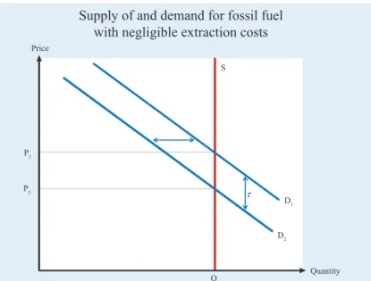
Let us consider the oil market based on the assump-tion that there is a finite amount of oil in the ground. Let us also, again only as a starting point, assume that the extraction cost is negligible relative to the value of oil. In the real world, the latter assumption is natural-ly violated, but the oil reserves of Saudi-Arabia satis-fy it reasonably well.
Figure 6.5 illustrates the situation just described. The supply of oil is vertical at Q, which is the amount existing in the ground. When interpreting this as rep-resenting the oil market, we should think of this sup-ply curve as representing the supsup-ply aggregated over all future time periods, rather than as the supply dur-ing an individual year.
The downward sloping line D1represents demand at
the outset. The price is P1and the quantity Q.Now
consider the effect of introducing a tax τon oil (or, equivalently, on the by-product of using it – CO2). At every market price excluding the tax, the demanded quantity is now lower. We can illustrate this as a shift downwards in the demand curve, where the shift downward is equal to the value of the tax. The new equilibrium is a price P2 that has the property that
τ
Supply of and demand for fossil fuel
with negligible extraction costs
Price S Q Quantity P1 P2 D1 D2 Figure 6.5 continued footnote 3:figure is in line with Grubb et al. (2006) who compare different estimates of the global cost of limiting climate change to tolerable levels. Their conclusion is that the cost is “unlikely to exceed one year’s foregone economic growth”. These figures indicate large yet arguably manageable costs, but they rely on policies being cho-sen in an optimal way.
4 Another argument, which is not dealt with in this chapter, is that energy systems often feature increasing returns to scale and network externalities. Thus, the pro-duction and/or delivery may be so called natural monopolies or feature very few suppliers, in which case it is well known that regulation may be needed to ensure economic efficiency.
P2+ τ = P1. The quantity remains at Q. As we see, the
price has fallen exactly as much as the tax, and the quantity has not changed.
In a dynamic model with the same features, it is straightforward to show that if a constant tax rate is introduced in every period, we obtain the same result as in the static example. Nothing happens to quanti-ties and the price falls in every period by a percentage amount equal to the tax rate. By deviating from the constant tax rate, the extraction pathmay be affected, but not the overall amount extracted. For example, a tax rate that falls over time induces resource owners to postpone extraction, i.e., to extract less today and more in the future.5
We can also analyse the effects of policies to reduce demand. Such policies can come in different forms. One such form is a unilateral policy that reduces demand in some, but not all, oil consuming coun-tries. Such a policy would shift demand inwards, resulting in a new, lower price. At this lower price, the additional demand from other countries exactly off-sets the reduction in demand in the countries that introduced the policy. The policy would then have no aggregate effect. This finding that reduc-tions in resource use in one region leads to an increase in other regions is sometimes called “leak-age”. In the case of an inelastic supply, we find complete leakage. Below we discuss a situation in which there is partial, but not complete leakage.
A result related to leakage occurs if non-fossil tech-nologies for energy production
are introduced. The effects of such policies can be analysed as a leftward shift in demand lead-ing to a lower price, but no change in quantity. A striking variant of this argument is the so-called “Green Para dox”, a term first coined by Hans-Werner Sinn in his book of the same title (Sinn 2012). Let us
assume that an alternative technology will replace fossil fuel at some point in the future. Let us suppose, furthermore, that this point is brought forward in time, thanks to a subsidised R&D program, for example. Thinking of the graph as representing
sup-ply and demand per period, we now have moreoil
per period to spend before the alternative becomes available – supply is shifted outward. Therefore, the price falls and extraction is accelerated.
So far we have discussed oil. The major threat to the climate is, however, not oil, at least not traditional, low extraction cost oil, but coal. BP (2010) reports that globally proved reserves of oil total 181.7 giga-tons. If this was the only fossil fuel to be burnt, cli-mate change would not be a worry. Adding this amount of CO2to the atmosphere would, according to standard estimates of climate sensitivity, be likely to lead to additional heating of well below one degree Celsius. However, there are large amounts of coal and other sources of fossil fuel that typically are fairly expensive to extract. Rogner (1997) estimates global reserves taking into account technical progress and ends up with an estimate of over 5,000 gigatons of oil equivalents. Burning even a small share of this reserve will most certainly be detrimen-tal for the climate.
With coal and non-traditional oil resources it is less reasonable to neglect extraction costs. IEA (2010) reports the average cost of producing coal at 43 US dollars per ton, while the average coal price 2005–2009 was 74 US dollars.6
τ
Supply of and demand for fossil fuel
with increasing extraction costs
Price S Q1 Q2 Quantity P1 P2 D1 D2 Figure 6.65 However, Hassler and Krusell (2011) recently showed that such a tax has both income effects and substitution effects. Under reasonable assumptions regarding preferences and technology, these effects can cancel each other out unless tax receipts are transferred to the resource owners (oil exporters). Taxing oil and giv-ing the proceeds to citizens of oil consum-ing countries then has no effect on the path of extraction, regardless of whether the tax is time-variant or not.
6 US Central Appalachian coal, see BP (2010).
Figure 6.6 illustrates an upward-sloping supply sched-ule for fossil fuel representing the case whereby more aggregate use requires the extraction of more costly resources. The interpretation of the figure is that the equilibrium determines how much fossil fuel will be used in total. If demand is given by D1, the total extracted volume will be Q1. Reserves with higher costs
will not be used, at least not as fuel. We see in the fig-ure that taxes and demand reductions now have an effect both on prices and quantities. A shift in the demand curve, regardless of the reason for the shift, affects the price as well as the quantity. In this case, unilateral demand reductions will lead to some leak-age, but this will not be complete. The “Green Paradox” will also be partly mitigated. The last unit extracted before the alternative technology takes over will have an extraction cost equal to its price. Reducing the time until the alternative fossil free technology becomes available leads to a reduction in the fossil fuel price. This has an effect on the total quantity extract-ed, but also speeds up extraction. A likely outcome is therefore higher emissions, but for a shorter period of time so that total emissions aggregated over time fall.
The conclusion of this section is that measures to reduce demand may be ineffective or even counter-productive. To analyse their effects, we need to model both supply and demand. Unfortunately and surpris-ingly, this point has been almost absent from policy discussion to date. We therefore currently have no clear indications as to the effects of policies like CO2 -taxes and emission quotas, in particular not of unilat-eral policies introduced by the European Union. It has so far been impossible to reach internationally binding agreements on CO2-reductions with wide cov-erage. Some positive signs have recently been seen, particularly the agreements reached during the United Nations Climate Change Conference in Durban in 2011, which may lead to agreements with more sub-stantial effects on global CO2-emissions.
6.3.2 The size of the climate externality
Great uncertainty surrounds the cost of emitting CO2. We simply do not know the exact dynamic mapping from CO2-emissions to climate change. Similarly, we do not know exactly which costs climate change will generate in the short or in the long run.
There are also several conceptual issues which do not have scientific answers, but require value judgments. Among them is the issue of how to compare costs and
benefits accruing to different individuals living in dif-ferent time periods or in difdif-ferent countries. Since the costs of climate change, as well as that of policies to mitigate or adapt to climate change, are unevenly spread over the world and over time, any aggregate number for the social costs of global warming explic-itly or implicexplic-itly relies on how these interpersonal comparisons are performed.
It is an inescapable fact that we do not and will not fully know the consequences of continuing to burn fossil fuel, or those of using alternative technologies to pro-duce energy. Despite this, decisions must be taken and these decisions should be based on the best knowledge available and with value judgments stated explicitly.
Fortunately, the number of studies on the social costs of emitting CO2is growing. Of course, these studies arrive at different numbers, but in total, they imply that we have valuable, albeit limited knowledge on which to base our calculations. Tol (2008) summaris-es the rsummaris-esult of 211 summaris-estimatsummaris-es of the social costs of car-bon emissions. Using the half of the sample that was published in peer-reviewed scientific journals, he finds that the mean of the estimates lies between 49 US dol-lars and 71 US doldol-lars, depending on the aggregation method used.7 The standard deviation is large and amounts to around two to four times the mean. Expressing these numbers in euros/tonCO2we arrive at values of between 10 and 14.8
There are many differences responsible for the differ-ent results in terms of the costs. However, as shown in Golosov et al. (2011), three separate factors are the key determinants of the social cost of emitting car-bon, namely:
• How long CO2is staying in the atmosphere.
• How much damage a given CO2-concentration
causes.
• How the welfare of future generations is dis -counted.
The first factor is largely determined by what is called carbon circulation, i.e., how carbon circulates between the atmosphere, the biosphere and the oceans. A good approximation of this according to IPCC (2007) and Archer (2005) is that a share of around 50 percent is absorbed quickly (within a few
7These numbers represent the purchasing power of US dollars in 1995.
8The mole weights of carbon and oxygen are 12 and 16, respective-ly. To get the cost per mass unit of carbon from the cost per mass unit of CO2, we therefore need to multiply by (2*16+12)/12=3.67.
decades) by plants and the upper layers of the oceans. One quarter stays for thousands of years while the remainder decays slowly, with a half-life of a few hun-dred years.
The second factor depends both on climate sensitivi-ty, i.e., how much climate change is caused by a change in CO2-concentrations, and how sensitive the economy is to climate change. It is a well-established fact that the direct greenhouse effect can be reliably approximated by a logarithmic function.9 A typical result from complicated climate models is that a dou-bling in CO2-concentrations leads to an increase of around three degrees Celsius in the global mean tem-perature. Given the logarithmic relationship, a qua-drupling of the CO2-concentration would then lead to an increase of six degrees. It is important to note that this means that a marginal increase in CO2 -concentra-tion has a smaller impact on the temperature the high-er the current CO2-concentration.
The most comprehensive quantitative investigation of the sensitivity of the economy to climate change to date is provided by Nordhaus (2008). Nordhaus find-ings imply that a marginal temperature rise has larger negative effects on the economy the higher the global mean temperature is. This finding, combined with the findings of the natural science literature mentioned above, implies that the marginal damage of a unit of emitted CO2is largely independent of how much has already been emitted.10This simplifies the calculation of marginal climate externalities substantially. Using these results, Golosov et al. (2011) show that the mar-ginal externality cost can be calculated with a very simple formula. The optimal tax in period tis:
The left-hand side is the tax per unit of emitted fossil carbon. On the right-hand side, Ytis global GDP in
period t, Et indicates that what comes after in the
expression may be uncertain and the expected values of these uncertain values should be used. ρis the sub-jective discount rate,11d(s) is the amount of a mar-ginal unit of emitted carbon that has left the atmos-phere after speriods and γmeasures the strength of the damage caused by climate change. As we see, new information about how long carbon stays in the atmosphere, how sensitive temperature is to CO2
-emissions or how much damage we should expect from a given temperature change can easily be incor-porated into the formula by changing γand the struc-ture of d(s).
Given a value of the externality, an optimal policy is easily devised. The conceptually simplest policy is to introduce a tax on emitted fossil carbon equal to the climate externality. As is seen in the formula, the externality is proportional to current global GDP. Therefore, as long as no new information about car-bon circulation or damages arrives, the tax per unit of emitted carbon should follow the development of world GDP. A tax equal to the externality is not the only possible optimal policy. An alternative is quan-tity restrictions, for example, by introducing a fixed number of emissions permits. The amount of such permits should then be set so that the price of the permit equals the climate externality. If more evi-dence emerges regarding the existence of so-called tipping points, where the climate becomes very sensi-tive to additional emission, the case for using emis-sion permits rather than taxes is strengthened since such a policy may make the emission volume easier to control.
Calibrating γ to the work on damages done by
Nordhaus (2008) and d(s)to recent work on the car-bon circulation, Golosov et al. (2011) compute the cli-mate externality per ton of fossil carbon emitted in the atmosphere as a function of the subjective dis-count rate ρ. The results, expressed in euros per ton of emitted fossil CO2 are shown in Figure 6.7. On the
x-axis different values of the subjective discount rate ranging from 0.1 percent per year to 3.4 percent per year are represented.
߬௧ൌ ܻ௧ܧ௧ሺͳ ߩሻି௦ሺͳ െ ݀ሺݏሻሻߛ ஶ
௦ୀ
9Feedback mechanisms are very important for the total effect. See footnote 9.
10There is certainly a great deal of uncertainty surrounding the assumptions behind this finding. More specifically, it is well known that the climate system has many non-linearities due to feed-back mechanisms. Examples include the melting of ice in the Arctic, Antarctica and Greenland. Since ice reflects sunlight better than sea water and ground, melting reinforces an initial increase in tempera-ture. Such non-linearities can even be strong enough to induce local-ly unstable dynamics. At some point, a minimal direct disturbance to the system then leads to a large discrete change. Such “tipping points” are analysed in Lenton et al. (2008) who find that, according to current knowledge, melting of ice on Greenland and in the Arctic are the most worrisome tipping points. If a consensus on such tip-ping points arises, the argument for limiting the temperature increase to levels below them is strengthened. Furthermore, it would make the social costs of carbon depend on current and expected future stocks of atmospheric CO2, invalidating the simple formula for the tax described in the main text.
11Note that this measures how much we prefer to consume at earli-er dates all else equal. It thearli-erefore compares the value of consuming equal amounts at different dates. The market discount (interest) rate, on the other hand, measures the value at actual consumption levels. When the economy and consumption grows, the market interest rate is higher than ρsince the future value of consumption is discounted for two reasons: the subjective time-preference captured by ρand since the value of a marginal unit of consumption is lower when con-sumption is higher.
Box 6.1
The optimal CO2-tax
Thisbox describesinsome detailtheequation determiningtheformulafortheoptimal CO2-tax giveninthetext.Theformularestson
strongsimplifyingassumptionsand should beconsidered asaback-of-the-envelopecalculation. Nevertheless,ittransparently demon
-strates keyconsiderationsbehind thecalculationofthesocialcostofcarbonemissions. Detailscanbefound in Golosov etal. (2011).
Firstly,consider howtomodelclimate damages. A typicalwayto dothisistoassumethatwecanassociateagivenincreaseintheglobal meantemperaturewith aformof damage,expressed asproportionallossofoutput. A commonfunctionalformforsuch a damagefunc
-tionis:
ܦሺܶሻ ൌ ͳ െ ͳ
ߠܶଶǤ
whereTistheincreaseintheglobalmeantemperatureand ߠisaparametercapturingthestrength ofthe damageeffect.Secondly,assume thatthetemperatureincreaseisafunctionofthecarboncontentintheatmosphere.Thelong-runresponseistypicallymodelled as:
ܶሺܵ௧ሻ ൌ ߣ ݈݊൬
ܵ௧
ܵ൰ ݈݊ʹǤൗ
Here,Stistheamountofatmosphericcarbonattimet.S0isthepreindustrialatmosphericcarboncontentand ߣisthesocalled climate
sensitivity.Thelatter quantifies howmuch heatingwegetfroma doublingofthecarboncontent. A typical valueisthree degrees Celsius.
Combiningthetwoequationsabove,wecanwritetheproportional damageasafunctionofthecarboncontentܦሺܶሺܵሻሻ. Golosov etal.
(2011)showthatthismappingisclosetolinearforreasonableparameters.ThiscomesfromthecombinationofD(T)beingconvex and T(S)concave.Thus,anincreaseintheamountofcarbonintheatmospherebyoneunit hasaconstantproportionaleffectonworld GDP.
Letus denotethatconstantwith theletterJ
Thenextconsiderationisthecarboncycle. When CO2isemitted intotheatmosphere,itentersacirculationsystem,wherecarbonflows
betweenthebiosphere,theatmosphereand theoceans. IPCC (2007)concludesthat: "About halfofa COpulsetotheatmosphereis removed overatimescaleof30years; afurther30percentisremoved withinafewcenturies; and theremaining20percentwilltypically stayintheatmosphereformanythousandsofyears" while Archer (2005)concludesthatagood approximationisthat75percentofan excessatmosphericcarbonconcentration hasameanlifetimeof300yearsand theremaining25percentstaysforever.Thiscanberepre
-sented byalinear deprecationstructured(s).The valued(s) describes howlargeashareofanemitted unitofcarbon haslefttheatmos
-phereaftersperiods.
Theoutputlossofaunitofcarbonemitted intimeperiod tincurred s 0periodsahead cannowbeexpressed as (d(s)JYt+s.Thefirst
term, (d(s)),captures howmuch oftheemitted carbonisleftintheatmosphereaftersperiods.Jdenotesthe damagesharecaused bya marginalunitofcarbonand Yt+sisoutputat datet+s.
Wecannoweasilypricethe damagebyexpressingthepresent discounted valueof damagescaused byaunitofcarbonemitted at
period t. Allowingforuncertainty,thisequals:
ܧ௧ ܴ௧௧ା௦ሺͳ െ ݀ሺݏሻሻߛܻ௧ା௦ ஶ
௦ୀ
whereEt denotesmathematicalexpectationsattimetand Rtt+sisthe discountfactortobeapplied betweenperiod tand t+s. Wecangofurtherthanthisbyusingthestandard macroeconomicresultthatthe discountfactorisgivenby:
ܴ௧௧ା௦ൌ ൬ ͳ ͳ ߩ൰ ௦ ݑԢሺܥ௧ା௦ሻ ݑԢሺܥ௧ሻ
whereݑԢሺܥሻisthemarginalutilityofconsumptionand Uisthesubjective discountfactor. Finally,letusassumethatutilityislogarithmic and thatconsumptionisaconstantfractionVofoutput,thenݑԢሺܥ௧ା௦ሻ ൌ ሺߪܻ௧ା௦ሻିଵ. Usingthisintheexpressionforthepresent discounted
valueofmarginal damagesyields:
߬௧ൌ ܻ௧ ൬ ͳ ͳ ߩ൰ ௦ ሺͳ െ ݀ሺݏሻሻߛ ஶ ௦ୀ
Plugging valuesforthe depreciationstructure (thed(s)’s),Jand currentworld outputforYtwearriveatanexpressionthatonly depends
onthesubjective discountrate.Theresultis depicted in Figure6.7.
Aswecansee,futureoutput doesnotenterintotheformulaforWt.Thisisimportantand theintuitionisstraightforward. Letussuppose
thatfutureoutputgoesupinsomeperiod. Inthatcase,since damagesceterisparibusareproportionaltooutput, damagesmeasured in outputinthatperiod increase. However,with increased output,consumptionalsoincreasesand thisreducestherelative valueofcon
-sumptionatthat date.Thesetwoeffectsexactlycancelout,leavingthepresent discounted valueof damagesconstant.
Finally,weshould notethattheformulareliesonstrongsimplifications.Theconsequencesofrelaxingthesimplificationsintheeconomic modelarefairlywell known. Movingawayfromlogarithmicutilityimpliesthatfuturegrowth ratesarenolongerneutralwith respectto thetax rate. With higherrisk aversion,a highergrowth rateleadstofasterfallingmarginalutilitiesand thusloweroptimaltax rates,for example. Distributionalissuesmayalsobeimportantand theabsenceofapossibilitytocompensateparticularly hard-hitregionsmaylead
toastrongerneed formitigationand highertaxes (seee.g., Hasslerand Krusell2011).Thepointofarguablythegreatestimportanceis thatstrongerconvexitiesinthemappingfromtemperatureto damagesmayimplythatoptimaltaxes depend onexpected futureemission pathsand thusalsoontechnologyand fossilfuelavailability (cf.alsofootnote9).
As we can see in the figure, the value of the climate externality and thus of the optimal tax, is sensitive to the value of the discount rate. This is easy to under-stand: much of a unit of emitted carbon stays in the atmosphere and causes potential damage for a very long time. The way we discount this future damage therefore strongly impacts the valuation of the stream of damage. For example, we see that if the discount rate is 1.5 percent per year, the optimal tax is 11 euros/ tonCO2. With a discount rate as low as 0.1 percent per year, the optimal tax is close to 100 euros/ tonCO2.
Currently, fossil fuel is taxed at quite different rates depending on who uses it. Gasoline for private use is typically the most heavily taxed. In addition to VAT, the average additional tax on
gasoline is 0.53 euros/liter. The lowest tax is applied in Cyprus at 0.35 euros/liter. and the high-est is levied in the Netherlands at 0.75 euros/liter. Ex pressing these numbers as a tax on CO2 -emissions12 yields the following numbers: the average tax is
227 euros/tonCO2, while in
Cyprus and the Nether lands the corresponding figures are 150 and 322. Of course, gasoline taxes have other purposes too like paying for roads, for
exam-ple, but it is instructive to make this comparison.
The European Union introduced an emission trading system in 2005. The system covers about half of the CO2emissions in the European Union and requires covered emitters to keep track of their emissions and annually deliver emission rights to the gov-ernment that equal their accumu-lated emissions. Since these emis-sion rights are traded on ex -changes, daily market prices can easily be observed.13The market price of emission rights has var-ied substantially since the intro-duction of the system. During the first year, it ranged between 20–30 euros/tonCO2. During the financial crisis, it fell dramatically and subsequently recovered during 2009 to a level of around 15 euros/tonCO2. Lately the price has fallen somewhat to a level of just above 10 euros/tonCO2.
The variability in emission prices is worrisome and may indicate that variability in demand for emission rights (fossil fuel) varies and that the elasticity of demand is low. A possible explanation for this is that industry demand for energy is very inelastic in the short run. In fact, energy is needed in quite fixed pro-portions to industrial output in the short run. A busi-ness cycle upturn may then increase the demand for energy and fossil fuel, causing a steep rise in the price
0 20 40 60 80 100 0.1 0.3 0.5 0.7 0.9 1.1 1.3 1.5 1.7 1.9 2.1 2.3 2.5 2.7 2.9 3.1 3.3
Optimal tax
as a function of the subjective discount rateSource: Golosov et al. (2011) and own calculations. Euros/ton CO2
discount rate in % per year Figure 6.7
Consequences of policy mistakes
Emission valueEmission value Emission value
Emission value Qh Ql Qh Ql Emission quantity Emission quantity Emission quantity Emission quantity Ph Pl Ph Pl Figure 6.8
12 A liter of gasoline contains around 0.63 kg of carbon producing about 2.33 kg of CO2.
13 See, e.g., http://www.eex.com,the web page of the European Energy Exchange.
of emission rights. Such business cycle variability is likely to be inefficient since the social costs of carbon are not sensitive to short run business cycle fluctua-tions. In fact, a low elasticity of demand for emission rights indicates that quantity restrictions of a cap-and-trade type have disadvantages relative to CO2-taxes.
Regardless of whether policy is formulated in terms of setting quantities (cap-and-trade) or prices (CO2 -taxes), we cannot trust that the policy formulation is exactly correct. However, the consequences of such mistakes are not necessarily independent of the type of policy used. This is illustrated in Figure 6.8. In the two upper panels we study the consequences of policy mistakes when the demand for emission rights is inelastic. The downward sloping curve rep-resents demand for emission rights and the upward sloping curve is the marginal social externality cost. The welfare maximising output is reached where the two curves cross and if the curves and policy are set optimally, this can be achieved either by allowing the right quantity of emission rights or using the right tax.
Let us now consider mistakes in policy. In the upper left panel, we consider two sub-optimal quantity restrictions indicated by the vertical dashed lines. One restriction is set too low and one too high. The social loss induced by such mistakes is given by the shaded area between the demand curve and the social cost curve. Let us now instead consider policy mistakes when taxes are used. For illustrative purposes, we take the size of the mistake to be the same. The two dashed horizontal lines indicate an excessively high and an excessively low tax respectively. Again, the welfare loss is the area between the two curves, which is shad-ed in the graphs. As we can see, the shadshad-ed areas are much smaller in the case where taxes are used as the policy instrument.
In the two lower panels, we repeat the experiment, but now assume that the elasticity is high. In this case, we see that our conclusions are reversed. Quantity restrictions lead to much smaller welfare losses. A similar exercise can be performed by changing the elasticity of the marginal social externality. In fact, our reasoning above indicates that the marginal social externality is close to constant, in which case the argu-ments above are strengthened. However, we need to reiterate that if more evidence on tipping points accu-mulates, this conclusion can be reversed. With strong tipping points, the marginal social externality is very sensitive to whether a marginal unit of emissions can
push the climate system over the tipping point. In such a case, quantity restrictions on emissions seem to be the more appropriate policy instrument.
A small number of countries in the European Union have introduced CO2-taxes on final consumers. In Sweden, this tax is approximately 100 euros/tonCO2. Finland, Denmark and Ireland have also introduced CO2taxes. Last year, the European commission pro-posed the introduction of a uniform European CO2 -tax of 20 euros/tonCO2. The proposal is that if this tax is introduced, other energy taxes should not be discriminatory against any particular source of ener-gy, but should only be based on energy content.
Let us finally discuss the issue of which discount rate to use. Here, one can use two lines of reasoning. The first is to use market data, for example, interest rates and average returns on shares. As noted in foot-note 10, these market rates are not the same as the subjective discount rates. Given a subjective discount rate, the market interest rate increases in line with eco-nomic growth. This reflects the fact that postponing consumption to a later date is worth less if consump-tion growth is high. Thus, market rates have to be adjusted by subtracting the effect of growth.14 Furthermore, insofar as risky market returns are used, a proper risk adjustment must be carried out. Doing these adjustments, typical estimates of ρ are in the range of 1–2 percent per year. This approach is advo-cated by Nordhaus (2008), for example.
A completely different approach is to argue that we cannot use market data to find proper values of the subjective discount rate. Instead moral judgments must be used, and these cannot justify such a high dis-count rate as is usually extracted from the market. This approach is proposed by the Stern report (Stern 2007), for example, which arrives at a discount rate of only 0.1 percent per year. Stern’s argumentation that we need to make moral judgments when it comes to valuing the effects on future generation has a clear appeal. However, one should note that if policies are to be based on a discount rate that is much lower than the rate that seems to exist in the market, interven-tions outside the area of climate policy may also be required. To the extent that capital accumulation is decided by market forces, savings and investment sub-sidies may be called for if the market discount rate is deemed to be too high.
14One can show that the market interest rate is equal to ρ + σg, where σis the inverse of the intertemporal elasticity of substitution and gis the growth rate of consumption. A widely-used assumption is that σ = 1 (logarithmic utility).
Although we appreciate that it may be possible to argue that we should use discount rates lower than the 1–2 percent that can be extracted from markets, we do believe that reasonable values for ρare spanned by the
x-axis in Figure 6.7. Given current knowledge of the consequences of global warming, it is then hard to
argue that CO2-taxes should be lower than
10 euros/tonCO2 or higher than 100 euros/tonCO2. Although this is a wide range, we can easily rule out several existing tax schemes as being too high and some as too low (particularly outside the European Union). It is also worth noting that in the calculations, we have not at all touched upon the fact that the European Union is only a small part of the world, par-ticularly when it comes to CO2-emissions. Existing studies do show that Europe may belong to a group of regions that are harder hit by climate change than oth-ers (like, for example, China and the United States). However, the externality costs calculated above are global and the cost of European emissions will largely fall on other regions. Perhaps more importantly, our calculations have not taken into account the fact that supply factors are critical to an understanding of the effect of taxes. Specifically, a unilateral introduction of a tax reduces demand and will lower world market prices. This increases the use of fossil fuels in the parts of the world that have not introduced the tax. Under some circumstances, this implies that a unilateral tax only shifts the use of fossil fuel from tax countries to the other countries, without affecting total use at all. This distorts world production and consumption with-out having any effect on the climate. This is the leak-age problem discussed above.15
6.3.3 The size of learning externalities
The second argument for why governments should intervene in the market for energy is that the develop-ment of new technologies may suffer from market failures since the benefits of improving technologies are seldom or never fully born by the developer of superior technologies. Relying fully on patents to pro-vide incentives to develop better technologies may, particularly in the case of green technologies, be prob-lematic or even counterproductive, since patents lead to high prices and less use of the improved technolo-gy. It may also be argued that in some cases, there are substantial amounts of non-propitiatory learning-by-doing that do not only benefit the doer. Some of the green technologies may arguably be in an early phase
of development where such an external learning curve is particularly steep.
It is clear that these two arguments in favour of poli-cies to promote green technologies are logical and rest on sound economic theory. However, they cannot be used to justify all policies favouring green technolo-gies. In particular, emitting one unit of CO2has a cost that is independent of how it was emitted. Conse -quently, reducing emissions by one unit has the same value regardless of how it is achieved. This value is certainly not fully known, but this does not change the argument that policies that work by putting a price on emissions should be neutral with respect to the way emissions are reduced. Such a “law of one price” is of key importance for economic efficiency, but is widely violated, as we will show below.
The argument that learning-by-doing externalities exist in some green technologies is a quantitative argu-ment. It is clear that learning externalities are differ-ent for differdiffer-ent technologies. The maturity of the technologies is a key factor behind differences in the size of the learning externality. In young technologies, there is more to be learnt than in old. Box 6.2 shows a simple quantitative example of how large subsidies for various green technologies can be motivated with learning externalities. Table 6.2 uses the IEA’s esti-mates of learning rates for different technologies to produce green electric power. The learning rate is defined as the cost reduction implied by a doubling of the installed capacity. This learning rate is highest for photovoltaic solar power (17 percent), but is negligi-ble for hydropower. It is reasonanegligi-ble to assume that part of these cost reductions are externalities. When one firm produces solar panels, the knowledge acquired cannot be completely appropriated by the individual firm. Instead, parts of the knowledge are dissipated to the industry as a whole. Thus, the incen-tive to accumulate such knowledge is weakened, cre-ating a cause for government intervention such as subsidies.
Table 6.2 shows the value of learning for different val-ues of learning rates and installed stocks of capacity. These values should be taken as upper bounds on the learning externality that would occur only in the hypothetical case when production is undertaken by a large number of producers, each so small that it has a negligible effect on total learning. In that case, a sub-sidy to investments represented by the numbers in the table can be justified. In reality, it is of course the case that many of the firms producing the different tech-15See also EEAG (2008), Chapter 5.
nologies are large enough to take into account their own effect on the learning curve. For example, the international wind turbine market is dominated by only a few manufacturers. There fore, the entries in the table are upper bounds on reasonable values of sub-sidisation. Never theless, the numbers in Table 6.2 are not very high.
Only in the case of photovoltaic solar power very early in the learning phase, is the upper bound on subsidy rates above one third.
Needless to say, our calculations should only be taken as a back-of-envelope attempt to judge what are reasonable ranges for subsidies based on the argument of learning externalities. Fur -thermore, they assume that introduction of the new technol-ogy is warranted, which is of course not necessarily the case. Instead, the cost of power gen-eration, taking into account the learning externality must be
compared across different production technologies and the cheapest should be chosen. Since there is learning, the currently cheapest technology is not necessarily the one with the lowest costs when learn-ing rates are taken into account. However, there are quantitative limits to this argument: even with the most generous assumptions on learning rates, like for photovoltaic electricity early in the development phase, current costs of more than twice the cost of the cheapest technology should not be accepted.
Box 6.2
Learning externalities and optimal subsidies
InIEA(2010)estimatesoflearningratesareprovided.Theselearningratesaredefinedasthepercentagereductionininvestment coststhatoccurastheinstalledcapacitydoubles.Ifthelearningrateis7percent(asisestimatedforonshorewind),adoublingof theinstalledcapacityreducesthecostby7percentwhileaquadruplingleadsto14 percentcostreductions.
GivenalearningrateG,wecanwritetheinvestmentcostattime t asafunctionofaccumulatedinstalledcapacityat t,denotedXt.Then, thecostfunctioncanbewritten
ሺܺ௧ሻ ൌ ሺܺሻሺͳ െ ߜሻ
ౢ൬బ൰ ౢሺమሻ,
whereሺܺሻisthecostatsomeinitialdate0andGisthelearningrate.Lettingxtbetheinvestmentrateattimet and r bea constantdiscountrate,thetotaldiscountedvalueofallfutureinvestmentcosts,givencurrent(period t)accumulatedinstalled capacityisthen: ܲሺܺ௧ሻ ൌ ݁ିሺ௦ି௧ሻ ஶ ௧ ሺܺ௦ሻݔ௦݀ݏ, whereܺ௧ൌ ܺ ݔ௦݀ݏ ௧
.Letusnowconsideraconstantinvestmentflowxnormalisedtounityandnormaliseሺܺሻ ൌ ͳǤThen
thenormaliseddiscountedvalueoffutureinvestmentcostsattime0is:
ܲሺܺሻ ൌ ݁ି௦
ஶ
ሺͳ െ ߜሻ
ౢሺ൬ೞశబబ൰ మ ݀ݏ.
Wecannoweasilycalculatehowmuchܲሺܺሻfallsforamarginalunitofextrainvestmentattime0fordifferentvaluesofthe
learningrate.Thisvaluedependsontheinitialstockofinstalledcapacity.Thisiseasytounderstand:agivenrateofinvestmenthasa largerrelativeimpactontheaccumulatedstockofcapacitythesmallerthelatteris.Thus,thelearningexternalityislarger,the small-erthestockofinstalledcapacityis.InTable6.2themarginalreductioninܲሺܺሻofaunitofextrainvestmentattime zerois
pre-sentedfordifferentlearningratesandfordifferentstocksofaccumulatedcapacity.Thediscountrateissetto 4 percentandthe learningratesaretakenfromIEA(2010,Table10.1).Thenumbersinthetablerepresentthediscountedvalueofthecostreductiona unitofinvestmentcausesrelativetothecostoftheinvestment.Take,forexample,solarphotovoltaiclearningrates,whichare esti-matedat17percentperdoublingofinstalledcapacity.Whenthestockofinstalledcapacityisequaltooneyearofinvestments,the valueoftheincurredcostreductionis50.8percentoftheinstallationcost.Afterfiveyears,thereductionhasfallento31.6percent. Thisisdiscussedinthemaintext.Thesenumberscanbetakenasupperboundsforthelearningexternalities.
Table 6.2
Cost reductions of future investments due to learning externalities in % of current investment costs
Learning rate
Installed capacity in terms of years of investment flow 1 5 10 20 Hydro, δ =0.01 4.0 2.1 1.5 1.0 Biomass, δ =0.05 18.4 10.3 7.4 4.9 Onshore windδ =0.07 24.8 14.2 10.2 6.9 Offshore wind, δ =0.09 30.8 17.9 13.0 8.8 Geothermal, δ =0.05 18.4 10.3 7.4 4.9 Solar photovoltaic, δ =0.17 50.8 31.6 23.5 16.3
Concentrated solar, δ =0.10 33.7 19.8 14.3 9.7 Source: IEA(2010) for learning rates and own calculations.
Instead, however, policy in many countries has been based on the principle that the costlier a particular technology is, the heavier it should be subsidised. This is absurd and inefficient.
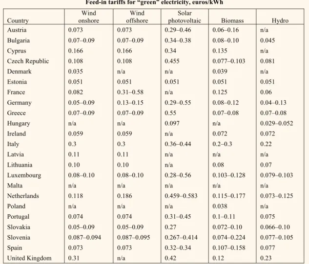
Table 6.3 shows current feed-in tariffs in EU coun-tries. These tariffs are what local small producers, typically households, receive if they produce electric-ity and “feed” it back to the electricelectric-ity grid. The tar-iffs are typically fixed over long-horizons so as to guarantee the return to investing in a technology that would not be profitable without the subsidy. The tar-iffs are very high, in many cases around 0.50 euros per kWh. As a comparison, the average production cost of wind power in the European Union is 0.06 euros per kWh (see EEA (2009), Table 6.7). The large sums spent on the subsidies implied by the high feed-in tariffs are, in the best of cases, simply a waste. However, they may very well also be directly counter-productive (Sinn 2012).
6.4 Conclusions
Let us now summarise the conclusions that can be drawn from this chapter in bullet form.
• Europe is heavily dependent on fossil fuel. Over the last two decades energy consumption has been roughly constant. The share of fossil fuel has been roughly constant at a high 80 percent with only a modest decline from 83 percent in 1990 to 77 per-cent in 2008. The share of energy generated by renewable sources has increased at a fairly high rate, almost doubling from 4.4 to 8.4 percent. If these trends continue, however, the EU target of 20 percent renewable energy by the year 2020 will not be reached until 2035.
• Targets regarding the share of renewable energy production set for individual member countries cannot be expected to ensure an efficient alloca-tion. The rule that individual countries can sell
Table6.3
Feed-intariffsfor “green” electricity, euros/kWh
Country Wind onshore Wind offshore Solar
photovoltaic Biomass Hydro
Austria 0.073 0.073 0.29–0.46 0.06–0.16 n/a Bulgaria 0.07–0.09 0.07–0.09 0.34–0.38 0.08–0.10 0.045 Cyprus 0.166 0.166 0.34 0.135 n/a Czech Republic 0.108 0.108 0.455 0.077–0.103 0.081 Denmark 0.035 n/a n/a 0.039 n/a Estonia 0.051 0.051 0.051 0.051 0.051 France 0.082 0.31–0.58 n/a 0.125 0.06 Germany 0.05–0.09 0.13–0.15 0.29–0.55 0.08–0.12 0.04–0.13 Greece 0.07–0.09 0.07–0.09 0.55 0.07–0.08 0.07–0.08 Hungary n/a n/a 0.097 n/a 0.029–0.052 Ireland 0.059 0.059 n/a 0.072 0.072 Italy 0.3 0.3 0.36–0.44 0.2–0.3 0.22 Latvia 0.11 0.11 n/a n/a n/a Lithuania 0.10 0.10 n/a 0.08 0.07 Luxembourg 0.08–0.10 0.08–0.10 0.28–0.56 0.103–0.128 0.079–0.103 Malta n/a n/a n/a n/a n/a Netherlands 0.118 0.186 0.459–0.583 0.115–0.177 0.073–0.125 Poland n/a n/a n/a 0.038 n/a Portugal 0.074 0.074 0.31–0.45 0.1–0.11 0.075 Slovakia 0.05–0.09 0.05–0.09 0.27 0.072–0.10 0.066–0.10 Slovenia 0.087–0.094 0.087–0.095 0.267–0.414 0.074–0.224 0.077–0.105 Spain 0.073 0.073 0.32–0.34 0.107–0.158 0.077 UnitedKingdom 0.31 n/a 0.42 0.12 0.23
excess renewable shares to countries that have not achieved their targets is good, but lacks credibility. • It is not at all clear that a policy to reduce fossil
fuel use unilaterally in the European Union has any effect at all on global emissions. By reducing demand in Europe, world market prices may fall, spurring higher use in other parts of the world. Gaining a better understanding of such leakage effects should be a top priority, along with finding ways of reaching binding agreements on mitigation policies with wide international coverage. • Provided that demand reductions in the European
Union have positive effects on global emissions, the CO2trading system is a way of efficiently allo-cating CO2-reductions. However, there may be rea-sons to consider a mechanism to stabilise prices. If the prices of permits are not in line with reasonable estimates of the social cost of carbon, volumes should be changed. The current rule that the owner of an emission right is allowed to save the right and use it at any later point is appropriate and may help to stabilise prices by increasing the demand for emission rights during business cycle downturns, for example, when fuel demand is low and may also increase the supply of emission rights when fuel demand is high.
• Based on current knowledge, the global social cost of emitting CO2 is likely to be in the range 10–100 euros/tonCO2. A more exact figure requires value judgments on how to value the welfare of future generations and greater knowledge of cli-mate change and its consequences. Implementing measures so that these costs are internalised is not likely to have a dramatic effect on the economy. However, poorly-constructed policy can easily lead to much higher costs, as well as smaller effects on climate change. A comprehensive climate policy for all EU member states is therefore necessary. • It is essential that policies are based on the
one-price principle.This principle states that the cost of reducing emissions by one unit should be the same regardless of how and where this is done. Policies that deviate from this like feed-in tariffs that make it several times more valuable to reduce emissions via solar panels on private houses than, for exam-ple, to use large offshore wind power farms, are very costly and hinder the technological develop-ment that could make us less fossil fuel dependent. Learning externalities may differ between different technologies, but are not large enough to motivate any substantially different treatment of them. Both different technologies and mitigation efforts, however, are currently treated inconsistently by
individual EU member states. The European Union should swiftly harmonise these policies. A first and simple step would be to introduce a com-mon CO2tax.
References
Archer, D. (2005), “The Fate of Fossil Fuel CO2in Geologic Time”,
Journal of Geophysical Research110, doi 10.1029/2004JC002625. Bretschger, L., Ramer, R. and F. Schwark (2011), “Growth effects of carbon policies: Applying a fully dynamic CGE model with heteroge-neous capital”, Resource and Energy Economics33, pp. 963–80. BP (2010), BP Statistical Review of World Energy,June,
http://bp.com/statisticalreview.
EEA (2009), Europe's onshore and offshore wind energy potential,
EEA Technical report No 6/2009, Copenhagen, Denmark, 2009. EEAG (2008), The EEAG Report on the European Economy, CESifo, Munich 2008, http://www.cesifo-group.de/DocDL/EEAG-2008.pdf.
Golosov, M., Hassler, J., Krusell, P. and A. Tsyvinski (2011), “Optimal Taxes on Fossil Fuel In General Equilibrium”, NBER Working Paper17348.
Grubb, M., Cavarro, C. and J. Schnellnhuber (2006), “Technological Change for Atmospheric Stabilization: Introductory Overview to the Innovation Modeling Comparison Project”, The Energy Journal,
Special Issue 2006, pp. 1–16
Hassler, J. and P. Krusell (2011), “Economics and Climate Change: Integrated Assessment in a Multi-Region World”, mimeo, IIES, Stockholm University.
IEA (2010), World Energy Outlook 2010, International Energy Agency, Paris, France, 2010.
IPCC (2007), “Climate Change 2007: The Physical Science Basis”, in: Metz, B., Davidson, O., Bosch, P., Dave, R. and L. Meyer (eds.),
Contribution of Working Group I to the Fourth Assessment Report of the Intergovernmental Panel on Climate Change, Cambridge University Press, Cambridge, United Kingdom and New York, NY, USA, 2007.
Lenton, T.M., Held, H., Kriegler, E., Hall, J.W., Lucht, W., Rahmstorf, S. and H.J. Schnellnhuber (2008), “Tipping elements in the Earth’s climate system”, Proceedings of the National Academy of Sciences105, pp. 1786–93.
Nordhaus, W., (2008), A Question of Balance: Weighing the Options on Global Warming Policies,Yale University Press, New Haven, 2008. Rogner, H.-H. (1997), “An Assessment of World Hydrocarbon Resources”, Annual Review of Energy and the Environment 22, pp. 217–62.
Sinn, H.-W. (2012), The Green Paradox,MIT Press, Cambridge, MA, 2012.
Stern, N. (2007), The Economics of Climate Change: The Stern Review,Cambridge University Press, Cambridge, United Kingdom, 2007.
Tol, R. (2008), “The Social Cost of Carbon: Trends, Outliers and Catastrophes”, Economics: The Open-Access, Open-Assessment E-Journal2, 2008-25.