Estimating Surface Soil Moisture from SMAP Observations Using a Neural Network Technique

(1)

Estimating surface soil moisture from SMAP

observations using a Neural Network technique

J. Kolassaa,b,∗, R.H. Reichleb, Q. Liuc,b, S.H. Alemohammadd, P. Gentined, K.

Aidae_{, J. Asanuma}e_{, S. Bircher}l_{, T. Caldwell}m_{, A. Colliander}f_{, M. Cosh}g_{, C.} Holifield Collinsn_{, T.J. Jackson}g_{, J. Mart´ınez-Fern´}_andezh_{, H. McNairn}i_{, A.}

Pachecoi_{, M. Thibeault}j_{, J.P. Walker}k

a_{Universities Space Research Association/NPP, Columbia, MD, USA}

b_{Global Modelling and Assimilation Office, NASA Goddard Spaceflight Center, Greenbelt,}

MD, USA

c_{Science Systems and Applications Inc., Lanham, MD, USA} d_{Columbia University, New York, NY, USA}

e_{University of Tsukuba, Tsukuba, Japan}

f_{Jet Propulsion Laboratory, California Institute of Technology, Pasadena, CA, USA} g_{USDA ARS Hydrology and Remote Sensing Laboratory, Beltsville, MD, USA} h_{Instituto Hispano Luso de Investigaciones Agrarias (CIALE), Universidad de Salamanca,}

Salamanca, Spain

i_{Agriculture and Agri-food Canada, Ottawa, Ontario, Canada}

j_Comisi`_{on Nacional de Actividades Espaciales (CONAE), Buenos Aires, Argentina} k_{Department of Civil Engineering, Monash University, Clayton, Victoria, Australia} l_{Centre d’Etudes Spatiales de la BIOsph`}_{ere (CESBIO-CNES, CNRS, IRD, Universit´}_e

Toulouse III), Toulouse, France

m_{University of Texas at Austin, TX, USA}

n_{USDA ARS Southwest Watershed Research Center, Tucson, AZ, USA}

Abstract

A Neural Network (NN) algorithm was developed to estimate global surface soil moisture for April 2015 to March 2017 with a 2-3 day repeat frequency using passive microwave observations from the Soil Moisture Active Passive (SMAP) satellite, surface soil temperatures from the NASA Goddard Earth Observing System Model version 5 (GEOS-5) land modeling system, and Moderate Res-olution Imaging Spectroradiometer-based vegetation water content. The NN was trained on GEOS-5 soil moisture target data, making the NN estimates consistent with the GEOS-5 climatology, such that they may ultimately be as-similated into this model without further bias correction. Evaluated against in

∗_{Corresponding author}

Email address: [email protected](J. Kolassa)

(2)

situ soil moisture measurements, the average unbiased root mean square error (ubRMSE), correlation and anomaly correlation of the NN retrievals were 0.037 m3m−3, 0.70 and 0.66, respectively, against SMAP core validation site measure-ments and 0.026 m3_m−3_{, 0.58 and 0.48, respectively, against International Soil} Moisture Network (ISMN) measurements. At the core validation sites, the NN retrievals have a significantly higher skill than the GEOS-5 model estimates and a slightly lower correlation skill than the SMAP Level-2 Passive (L2P) product. The feasibility of the NN method was reflected by a lower ubRMSE compared to the L2P retrievals as well as a higher skill when ancillary parameters in physically-based retrievals were uncertain. Against ISMN measurements, the skill of the two retrieval products was more comparable. A triple collocation analysis against Advanced Microwave Scanning Radiometer 2 (AMSR2) and Advanced Scatterometer (ASCAT) soil moisture retrievals showed that the NN and L2P retrieval errors have a similar spatial distribution, but the NN retrieval errors are generally lower in densely vegetated regions and transition zones.

Keywords: soil moisture remote sensing, SMAP, data assimilation, microwave

radiometer

1. Introduction 1

Soil moisture is a key variable for many surface and boundary layer

pro-2

cesses, such as the coupling of the water and energy cycles (Seneviratne et al.,

3

2006;Gentine et al., 2011;Bateni and Entekhabi, 2012) or the partitioning of

4

precipitation into runoff and infiltration (Philip, 1957; Corradini et al., 1998;

5

Assouline, 2013). Soil moisture is also a key determinant of the carbon cycle

6

(McDowell, 2011; Sevanto et al., 2014; Jung et al., 2017). The importance of

7

soil moisture has been recognized by the World Meteorological Organization by

(3)

naming it an Essential Climate Variable (GCOS, 2009) and thus encouraging

9

efforts to obtain better soil moisture observations, which is challenging because

10

of its high variability both in space and time.

11

One avenue to obtain observations of soil moisture is through satellite

instru-12

ments that provide global observations with a relatively short revisit period of

13

2-3 days. In particular, L-band (1.4 GHz) microwave instruments exhibit a high

14

sensitivity to soil moisture in the top∼5 centimeters of the soil in sparsely to

15

moderately vegetated areas. This has led to the launch of two L-band satellite

16

missions to observe soil moisture, the European Soil Moisture and Ocean

Salin-17

ity (SMOS) mission in 2009 (Kerr et al., 2010) and the NASA Soil Moisture

18

Active Passive (SMAP) mission (Entekhabi et al., 2010) in 2015.

19

Traditionally, satellite soil moisture retrievals from L-band (and other)

sen-20

sors are implemented through the inversion of Radiative Transfer Models (RTMs)

21

(e.g. Owe et al.(2001);Kerr et al.(2012);O’Neill et al.(2015)), which

explic-22

itly formulate the physical relationships linking surface soil moisture to satellite

23

brightness temperature observations. The RTM inversion technique is used to

24

produce the official SMOS and SMAP retrieval products, and is able to provide

25

high quality soil moisture estimates (Al Bitar et al., 2012;Chan et al., 2016b;

26

Colliander et al., 2017) with a typical latency of 12 to 24 hours. However, this

27

approach requires accurate knowledge of the physical relationships between the

28

surface state and the satellite observations as well as their associated

parame-29

ters, which are often empirically estimated and thus uncertain. Moreover, RTM

30

inversions also require explicit information on other surface states, including

(4)

surface soil temperature and vegetation, and are thus typically ill-posed

prob-32

lems. Additionally, for time critical applications, such as near real time flood

33

prediction or soil moisture assimilation into weather prediction models, retrieval

34

products with a shorter latency are required.

35

Data assimilation provides another option to generate improved soil moisture

36

estimates through the merging of satellite and model information, and can yield

37

soil moisture estimates that are of higher quality than estimates from satellite

38

observations or models alone (e.g. Entekhabi et al.(1994);Walker and Houser 39

(2001); Liu et al. (2011); Lahoz and De Lannoy (2014)). For soil moisture

40

assimilation, the observations and model estimates have to be unbiased with

41

respect to each other, which is typically achieved by locally matching the mean

42

and variability of the satellite observations to those of the model (Reichle and 43

Koster, 2004). While this satisfies the requirements of the assimilation system,

44

it has the side effect of removing some independent information in the satellite

45

observations. Given the high quality of soil moisture observations from SMOS

46

and SMAP this is undesirable.

47

As an alternative to RTM inversions, statistical Neural Network (NN)

re-48

trieval algorithms have been successfully implemented for a number of sensors

49

in recent years (Aires et al., 2005;Chai et al., 2009;Kolassa et al., 2013, 2016;

50

Rodriguez-Fern´andez et al., 2015;Santi et al., 2016). Instead of explicitly

for-51

mulating physical relationships, NNs are calibrated on a sample of satellite

ob-52

servations and corresponding soil moisture estimates (the target data) to model

53

the global statistical relationship between the satellite observations and surface

(5)

soil moisture. As a result, NN retrievals can offer several general advantages

55

over traditional RTM inversions. First, they do not require an explicit

param-56

eterization of physical relationships and are thus not affected by errors in our

57

knowledge of these relationships or their parameters. Second, after a one-time

58

calibration, NNs are computationally extremely efficient and can provide soil

59

moisture estimates almost immediately after arrival of the instrument data,

60

thereby shortening the latency. Third, training a NN non-locally on target data

61

from a model, yields NN retrievals that are globally unbiased with respect to

62

the model, with spatial and temporal patterns that are driven by the satellite

63

observations (e.g. Jimenez et al.(2013);Kolassa et al.(2016);Alemohammad et 64

al.(2017)). This may reduce the need for bias correction prior to an assimilation

65

and at the same time retain more of the independent information contained in

66

the spatial and temporal patterns of the satellite observations.

67

In this study, we develop the first NN algorithm to retrieve global surface

68

soil moisture from SMAP observations. The motivation for this work is

two-69

fold. First, we investigate statistical retrieval techniques as a possible

alterna-70

tive or supplement to the existing physically-based SMAP retrieval algorithms.

71

Since statistical techniques require less ancillary data and are subject to

differ-72

ent algorithm-related errors than physically-based retrievals, NN retrievals may

73

provide useful information where and when RTMs are known to be uncertain.

74

For SMOS, the NN technique has been successfully implemented ( Rodriguez-75

Fern´andez et al., 2015). However, it is not obvious that a NN for SMAP will

76

work equally well, given the differences between SMOS and SMAP in the

(6)

serving geometry (multiple vs. single incidence angle) and instrument error

78

characteristics (De Lannoy et al., 2015). Second, we aim to investigate the

79

potential of statistical techniques to generate a soil moisture product with

char-80

acteristics beneficial to SMAP soil moisture assimilation. The NN algorithm

81

retrieves soil moisture in the climatology of the target model and thus may

82

reduce the need for bias correction prior to data assimilation. In a follow-on

83

study, we will investigate whether this results in a more efficient use of SMAP

84

observations during data assimilation.

85

The NN retrieval algorithm is trained with SMAP brightness temperatures

86

and two ancillary datasets as inputs, and with target data from the NASA

God-87

dard Earth Observing System version 5 (GEOS-5) model (section 2). Using the

88

trained NN, we compute global estimates of volumetric surface soil moisture

89

for the period April 2015 to March 2017 and evaluate them using a number of

90

different metrics and techniques (section 3). We compare the SMAP NN soil

91

moisture estimates to the target GEOS-5 model soil moisture to identify the

in-92

dependent information provided by the SMAP observations that can potentially

93

inform the model during data assimilation (section 4.1). Next, we assess the

94

SMAP NN retrievals against independent in situ measurements and compare

95

their skill to that of the SMAP Level-2 passive (L2P) retrieval product and the

96

GEOS-5 model soil moisture (section 4.2). Finally, we assess the global error

97

distributions of the SMAP NN, GEOS-5 and SMAP L2P products using a triple

98

collocation (TC) analysis in conjunction with soil moisture retrievals based on

99

observations from the Advanced Microwave Scanning Radiometer 2 (AMSR2)

(7)

and the Advanced Scatterometer (ASCAT), which have independent errors with

101

respect to the SMAP and GEOS-5 products (section 4.3).

102

2. Datasets 103

2.1. Neural Network Inputs and Target Datasets 104

2.1.1. SMAP Observations 105

The main input to the NN soil moisture retrieval algorithm are the SMAP

106

brightness temperatures. SMAP was launched in January 2015 and is equipped

107

with an L-band (1.4 GHz) radiometer observing on four different channels,

hor-108

izontal and vertical polarization as well as the 3rd and 4th Stokes’ parameter.

109

SMAP is in a sun-synchronous, near-circular orbit with equator crossings at 6

110

AM and 6 PM local time and a revisit time of 2-3 days (Entekhabi et al., 2010).

111

Brightness temperature data have been collected since 31 March 2015.

112

For our NN retrieval product we use SMAP Level-1C brightness

temper-113

atures (Chan et al., 2016a) for the April 2015 to March 2017 period. The

114

data are provided on the 36-km resolution Equal-Area Scalable Earth version

115

2 (EASEv2) grid (Brodzik et al., 2012) as daily half-orbit files. We only use

116

observations from the 6 AM overpass, in order to minimize observation errors

117

due to Faraday rotation and the difference between the soil and canopy

tem-118

peratures (Entekhabi et al., 2010;O’Neill et al., 2015). A test of different input

119

combinations indicated that using data from all four SMAP channels as

in-120

puts to the retrieval algorithm yielded the best NN retrieval performance (not

121

shown). While the 3rd and 4th Stokes’ parameters are not directly sensitive to

(8)

soil moisture, including them as inputs helps the NN algorithm to distinguish

123

between different observing conditions and thus determine the weight for a given

124

brightness temperature observation.

125

2.1.2. GEOS-5 Model Surface Soil Moisture and Temperature 126

The model soil moisture estimates used here are generated using the

GEOS-127

5 Catchment land surface model (Koster et al., 2000; Ducharne et al., 2000).

128

The Catchment model version used in this study is very similar to that of the

129

SMAP Level-4 Soil Moisture (L4 SM) version 2 system (Reichle et al., 2015,

130

2016, 2017b(in press), but SMAP brightness temperature observations are not

131

assimilated. The surface meteorological forcing data were provided at 0.25◦ 132

resolution by the GEOS-5 Forward Processing atmospheric data assimilation

133

system (Lucchesi, 2013). The GEOS-5 precipitation forcing data were

cor-134

rected using global, daily, 0.5◦ resolution, gauge-based observations from the

135

Climate Prediction Center Unified (CPCU) product, which have been scaled to

136

the Global Precipitation Climatology Project (GPCP) v2.2 pentad

precipita-137

tion product climatology (Reichle and Liu, 2014; Reichle et al., 2017a,b). The

138

GEOS-5 background precipitation was also scaled to the GPCP v2.2

climatol-139

ogy. Output fields were produced as 3-hourly time averages and provided on

140

the 9-km EASEv2 grid.

141

In this study, we use two model output fields: (1) the surface soil moisture

142

(0-5 cm soil layer) and (2) the surface soil temperature (0-10 cm soil layer). The

143

GEOS-5 soil moisture fields served as target data in the NN training (section

(9)

retrieval compared to that of the target model. The surface soil temperature

146

data were used as an input to the retrieval algorithm to account for the surface

147

soil temperature contribution to the observed brightness temperatures (section

148

3.1). Using surface soil temperature estimates from the target model potentially

149

introduces some of the GEOS-5 spatial patterns into the NN estimates and could

150

lead to model dependency issues during a later assimilation of the NN estimates

151

into the GEOS-5 model. The same would be true, however, for the assimilation

152

of the SMAP L2P product, which also uses GEOS-5 ancillary soil temperatures

153

(section 2.2.1). We assume here that the canopy temperature and surface soil

154

temperature are in equilibrium for the 6 AM (local time) SMAP observations

155

used here, so only a single temperature estimate is required. The surface soil

156

temperature data were also used in the data quality control to identify frozen

157

soil conditions (section 2.3).

158

2.2. Validation Datasets 159

2.2.1. SMAP Level-2 Passive Retrievals 160

The SMAP L2P soil moisture retrieval product uses SMAP radiometer

Level-161

1C brightness temperatures to provide soil moisture estimates on the 36-km

EA-162

SEv2 grid as daily half-orbit files. The retrieval algorithm is based on a physical

163

tau-omega model (Wigneron et al., 1995;O’Neill et al., 2015) to isolate the soil

164

emission from the total observed surface emission (soil and vegetation) and to

165

subsequently convert it into a soil moisture estimate through the use of soil

166

emission and mixing models. The surface soil temperature data required by

167

the tau-omega model are provided by the quasi-operational GEOS-5 Forward

(10)

Processing system (Lucchesi, 2013) with a 0.25◦ resolution. The tau-omega

169

model also requires information on the vegetation water content (VWC), which

170

is estimated from a climatology of the Normalized Difference Vegetation Index

171

based on Moderate Resolution Imaging Spectroradiometer (MODIS)

observa-172

tions using an empirical relationship established from prior investigations. No

173

retrieval is performed for frozen soil conditions based on GEOS-5 surface soil

174

temperature. Soil moisture retrievals are flagged as ‘not recommended’ when

175

the VWC within the satellite footprint exceeds 5 kg m−2 ₍_{O’Neill et al.}_{, 2015).}

176

In this study, we use version 4 of the L2P ‘baseline’ soil moisture estimates

177

derived from the SMAP morning (6 AM) overpass vertical polarization

bright-178

ness temperatures (O’Neill et al., 2016). Only data points flagged as having the

179

‘recommended’ retrieval quality were used.

180

2.2.2. AMSR2 and ASCAT Soil Moisture Retrievals 181

The Advanced Multichannel Scanning Radiometer 2 (AMSR2) is a

multi-182

channel passive microwave satellite instrument that has been collecting data

183

since July 2012. AMSR2 measures brightness temperatures at frequencies

rang-184

ing from 6.9 GHz to 89 GHz with a revisit time of approximately 2 days and

185

equator crossings at 1.30 AM and 1.30 PM local time (Kasahara et al., 2012).

186

Here we use the Japan Aerospace Exploration Agency AMSR2 soil moisture

187

product computed from the 10.7 GHz and 36.5 GHz vertical and horizontal

188

polarization brightness temperatures (Maeda and Taniguchi, 2013). The data

189

are provided as daily estimates of volumetric surface soil moisture on a grid

(11)

The Advanced Scatterometer (ASCAT) (Figa-Salda˜na et al., 2002) is an

192

active microwave satellite instrument aboard the MetOp satellites, which have

193

been collecting data since 2006. ASCAT measures surface backscatter at

C-194

band (5.3 GHz) with a revisit time of 1-2 days and equator crossings at 9.30

195

AM and 9.30 PM.

196

Here we use the ASCAT surface soil moisture product developed byWagner 197

et al. (2013). The data are provided in units of surface degree of saturation

198

with a sampling distance of 12.5 x 12.5 km and were converted into estimates

199

of volumetric surface soil moisture using the soil porosity data ofReynolds et 200

al.(2000).

201

Despite being posted on finer resolution grids, the spatial resolution of the

202

AMSR2 and ASCAT observations is very similar to the SMAP 36-km resolution.

203

2.2.3. In Situ Measurements 204

SMAP Core Validation Sites. The SMAP core validation sites (referred to here

205

as ‘core sites’) represent locally dense networks of in situ soil moisture

measure-206

ments that are specifically designed for the calibration and validation of SMAP

207

soil moisture products (Colliander et al., 2017). Each site features an array of

208

soil moisture sensors to represent the different spatial scales of the SMAP

prod-209

ucts (3 km, 9 km and 36 km). The measurements from each site’s sensors are

210

combined into and area-weighted average to yield one soil moisture time series

211

per site that is representative of a 36-km satellite grid cell.

(12)

1: Ov erview of the SMAP Cal/V al cor e sites. Sho wn are (from left to ri g h t) the site name, reference pixel ID (RPID ), lo cation, climate, la nd v er an d the a v era ge n um b e r of senso rs that co n tribute to the reference pixel a v erage. Soil moisture is measured at 5 cm depth or o v er the top 5 ( Col liander et al. , 2017) Site (abbreviation) RPID lo cation climate land co v er n um b er of sensors REMEDHUS (RM) 03013602 Spain temp erate cro plands 14 Reynolds Creek (R C) 04013601 USA (Idaho) arid grasslands 5 Y anco (YC) 07013601 Australia arid croplands 26 Carman (CM) 09013601 Canada cold croplands 19 Tw en te (TW) 12043602 Holland temp erate croplands / natural mosaic 9 W aln ut Gulc h (W G) 16013603 USA (Arizona) arid shrub op en 20 Little W ashita (L W) 16023602 USA (Oklahoma) temp erate grasslands 16 F ort Cobb (F C) 16033602 USA (Oklahoma) temp erate grasslands 12 Little Riv er (LR) 16043602 USA (Georgia) temp erate croplands / natural mosaic 19 South F ork (SF) 16073602 USA (Io w a ) cold croplands 18 Mon te Buey (MB) 19023601 Argen tin a temp erate croplands 10 Kenaston (KN) 27013601 Canada cold croplands 26 TxSON (TX) 48013601 USA (T exas) temp erate grasslands 32 Mahasri (MH) 53013601 Mongolia cold g rasslands 5

(13)

YC MH TW RM LR SF CM KN RC FC LW WG _TX MB Figure 1: Lo ca tion of the SMAP core v alidation sites (blue circles) and ISMN stations (red crosses). The bac kground sho ws the dominan t In ternational Geosphere-Biosphere Program (IGBP , ( Belwar d et al. , 1999)) land co v er class for eac h lo cation.

(14)

Table 1 summarizes the main characteristics of the 36-km core sites used

213

here. Out of the 14 locations, nine are in North America, two in Europe, and

214

one each in Asia, Australia and South America. The sites represent a range

215

of different climatic conditions and land cover types, and the average number

216

of sensors that contribute to the 36-km reference pixel data ranges between

217

5 and 32. Figure 1 shows the distribution of the SMAP core sites and their

218

corresponding dominant land cover.

219

International Soil Moisture Network (ISMN). 220

(15)

T able 2: Ov erview of the ISMN ( Dorigo et al. , 2011). Sho wn are the lo cation, n um b er of stations p er net w ork and the net w ork-sp ecific reference. Net w ork lo catio n # stations reference Dahra Senegal 1 ( T agesson et al. , 2015) FMI Finland 27 ( Dorigo et al. , 2011) iR ON USA 6 ( T aylor e t al. , 2015) PBO H2O USA 161 ( L arson et al. , 2008) REMEDHUS Spain 24 ( Sanchez et al. , 2012) RSMN Romania 20 ( Dorigo et al. , 2011) SCAN USA 181 ( Schaefer et al. , 2007) SMOSMANIA F rance 21 ( Calvet et al. , 2007) SNOTEL USA 441 ( L eavesley et al. , 2008) SOILSCAPE USA 171 ( Mo ghaddam et al. , 2016) USCRN USA 115 ( Diamond et al. , 2013 )

(16)

We further evaluate the NN retrieval product against independent in situ soil

221

moisture measurements from the International Soil Moisture Network (ISMN),

222

a database of soil moisture networks hosted at the Technical University (TU)

223

of Vienna (Dorigo et al., 2011) and referred to here as the ‘sparse networks’.

224

We used only ISMN networks that are not part of the SMAP core sites (Table

225

2). The REMEDHUS network comprises a different set of sensors for the core

226

site and as a sparse network and thus appears for both in situ data types. The

227

measurement depth, repeat frequency, coverage, station density and

measure-228

ment method depend on the contributing network. The number of stations in

229

each network ranges between 1 and 441 (Table 2), but - unlike for the core sites

230

- there is typically only one sensor per 36-km grid cell. That is, the ISMN

mea-231

surements are not necessarily representative of the spatial scale of the satellite

232

observations. Figure 1 shows the spatial distribution of the ISMN stations and

233

the dominant land cover at each location.

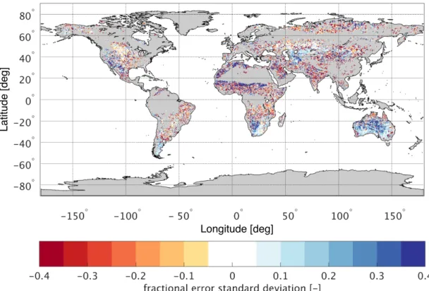
234

For two of the ISMN networks, SCAN (Schaefer et al., 2007) and USCRN

235

(Diamond et al., 2013), the data were already available in-house and had been

236

subjected to additional quality control as described inDe Lannoy et al. (2014)

237

and (Reichle et al., 2015b) (their Appendix C). Hence, the in-house data were

238

used for SCAN and USCRN instead of the data provided through the ISMN. As

239

a result, more reliable metrics could be estimated for these two sparse networks.

(17)

2.3. Data Preprocessing 241

2.3.1. Satellite Observations and Model 242

We co-located all datasets spatially and temporally, using the 36-km EASEv2

243

grid and the SMAP morning (6 AM) overpass times as a reference. The GEOS-5,

244

AMSR2 and ASCAT data were aggregated from their higher-resolution native

245

grids to the 36-km EASEv2 grid using simple averaging. The temporal

co-246

location was implemented by using the GEOS-5 3-hourly average that includes

247

the SMAP morning overpass for a given location and day. For the AMSR2 and

248

ASCAT retrieval products, only data from their night-time/morning overpasses

249

for the same day - at 1.30 AM and 9.30 AM, respectively - were used since

250

these are closest in time to the SMAP overpass at 6 AM. Likewise, for the L2P

251

retrievals we used only the morning overpass estimates, and no regridding was

252

required because the SMAP-based NN and L2P products are provided on the

253

same 36-km EASEv2 grid.

254

We additionally applied several quality control steps to the satellite and

255

model data sets to identify and exclude conditions in which a soil moisture

re-256

trieval was not feasible. Using the GEOS-5 surface soil temperature, we excluded

257

times and locations with a surface soil temperature below 1◦_{C. The} MODIS-258

based VWC estimates provided with the L2P data were used to exclude times

259

and locations with a VWC higher than 5 kg m−2_{, where the SMAP radiometer}

260

is not expected to provide reliable retrievals. Finally, we excluded all pixels

261

within 72 km of a water body - defined as a grid cell with a water fraction in

262

excess of 5% according to the GEOS-5 land mask - to mitigate the impact of

(18)

water bodies, as their low brightness temperatures cause erroneously high soil

264

moisture retrievals (O’Neill et al., 2015).

265

2.3.2. In Situ Data 266

The core site measurements are representative of the 36-km spatial resolution

267

of the retrievals and the aggregated model, however, the geographical center of

268

the in situ sensors for a given reference pixel does not generally coincide with

269

the EASEv2 grid cell center of the satellite and model products. Similarly,

270

the location of a (single point) ISMN measurement is typically offset from the

271

center of a EASEv2 grid cell. To account for this, the retrieval and (aggregated)

272

model soil moisture were linearly interpolated to the in situ location using data

273

from the nearest EASEv2 grid cell and its 8 surrounding neighbors, requiring a

274

minimum of 4 data points. Where applicable, ISMN measurements located in

275

the same EASEv2 grid cell were averaged and their average location was used

276

for the interpolation. For each day, the in situ measurement closest in time and

277

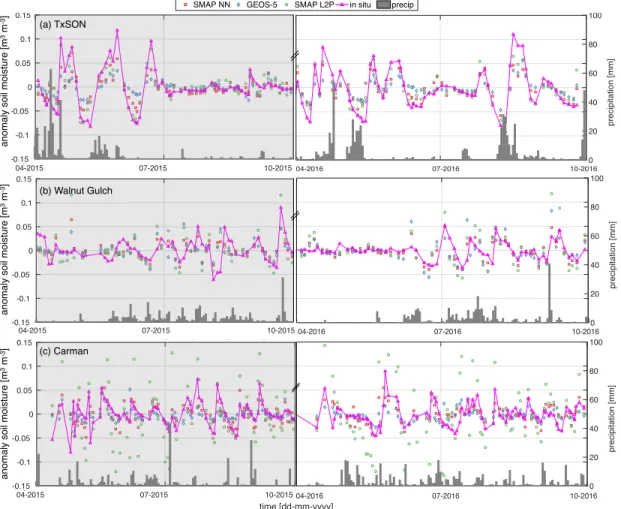
within a 3 hour window of the SMAP overpass was used.

278

Using the GEOS-5 surface temperature for the ISMN measurements and the

279

in situ surface soil temperature observations for the core site measurements, the

280

in situ data were screened for (nearly) frozen soil conditions by applying the

281

same 1◦C threshold that was used for the satellite and model data.

(19)

3. Methodology 283

3.1. Neural Network Retrieval Algorithm 284

In this study we use a NN approach to retrieve global surface soil

mois-285

ture with a 2-3 day repeat using SMAP brightness temperatures, GEOS-5 soil

286

temperatures and the MODIS-based VWC climatology that is used in the

gener-287

ation of the SMAP L2P product. The NN retrieval algorithm is first calibrated

288

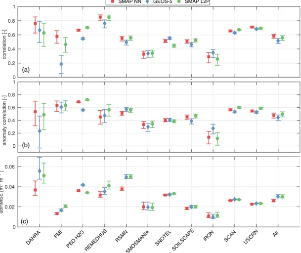
(trained) using a subset of the available SMAP and model data to determine the

289

statistical relationship between the satellite observations and surface soil

mois-290

ture. Once calibrated, the trained NN is used to retrieve surface soil moisture

291

from the entire set of satellite observations.

292

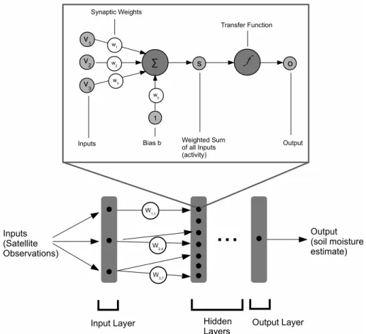
3.1.1. Neural Network Architecture 293

A neural network is a group of computational nodes arranged in a layered

294

and inter-connected architecture. Figure 2 shows a schematic of a basic NN for

295

soil moisture retrievals. The NN used here consists of 3 layers: (1) an input layer

296

that receives the satellite observations and ancillary inputs, (2) one hidden layer,

297

and (3) an output layer that produces the soil moisture estimates. This

archi-298

tecture is sufficient to approximate any continuous function (Cybenko, 1989).

299

The inputs for the SMAP NN retrieval algorithm are the observations from the

300

four SMAP channels, the GEOS-5 surface soil temperature and the

MODIS-301

based VWC estimates. The output from the NN algorithm is an estimate of the

302

volumetric surface soil moisture.

303

While the number of neurons in the input and output layers is determined by

(20)

Inputs (Satellite Observations) Output (soil moisture estimate)

...

Input Layer Hidden

Layers Output Layer

W_1,1 W_3,7 W_2,4 ∑ v 1 v₂ v 3 s

f

o w₁ w₂ w3

Inputs Weighted Sum _{of all Inputs} (activity) Output 1 wb Bias b Synaptic Weights Transfer Function

Figure 2:Schematic of a neural network with close-up of a single neuron (adapted from

(21)

the number of input and output variables (here, 6 for the input layer and 1 for

305

the output layer), the optimal number of neurons in the hidden layer depends on

306

the problem complexity. We found that for this study 15 hidden layer neurons

307

constituted the lowest number of neurons that was able to converge to a solution

308

during the NN training. We use a fully connected feed-forward network, in which

309

all neurons from one layer are connected to all neurons in the next layer. These

310

connections are assigned weights - the synaptic weights - used by each neuron

311

to compute a weighted sum of all its input plus a bias before applying a transfer

312

function. Neurons in the input and output layers use a linear transfer function,

313

while hidden layer neurons use the typical tangent-sigmoid transfer function.

314

3.1.2. Neural Network Training 315

In order to determine the statistical function that relates the NN input

316

data, including the satellite brightness temperature observations, to surface soil

317

moisture, the NN is calibrated on a sample set of NN inputs and coincident soil

318

moisture estimates (the target data), together referred to as the training data.

319

This process is referred to as the NN training and is schematically illustrated

320

in Figure 3 (a). To generate a training dataset representative of all expected

321

conditions, we used the first year (April 2015 - March 2016) of our study period

322

for NN training. The second year (April 2016 - March 2017) of the study

323

period was used for the evaluation presented in sections 4.1 and 4.2. Model

324

soil moisture estimates from GEOS-5 are used as the target data, because (1)

325

the model estimates have a similar resolution as the satellite observations while

326

providing complete spatio-temporal coverage and (2) training on a model yields

(22)

(a) NN Training

(b) Soil Moisture Estimation SMAP Tbv, Tbh, Tb3, Tb4, GEOS-5 T_s, MODIS VWC (NN input) Soil moisture (NN output) GEOS-5 soil moisture (target data) Neural Network Estimate MSE Training Goal met? Maximum # iterations? Overfitting? Update NN weights Stop Training Yes Yes Yes No No No Quality Control Retrieval

(NN) inputs Soil Moisture(NN output)

Trained Neural Network SMAP Tb_v, Tb_h, Tb₃, Tb₄, GEOS-5 T_s, MODIS VWC (NN input) Quality Control

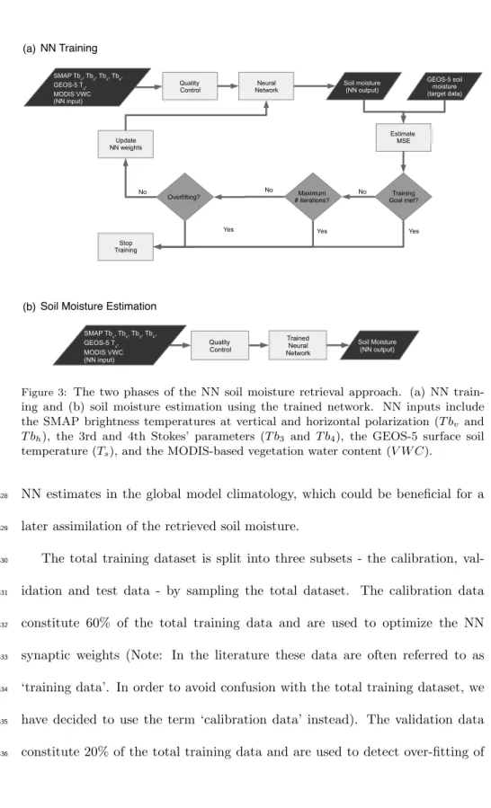
Figure 3: The two phases of the NN soil moisture retrieval approach. (a) NN

train-ing and (b) soil moisture estimation ustrain-ing the trained network. NN inputs include

the SMAP brightness temperatures at vertical and horizontal polarization (T bv and

T bh), the 3rd and 4th Stokes’ parameters (T b3 and T b4), the GEOS-5 surface soil

temperature (Ts), and the MODIS-based vegetation water content (V W C).

NN estimates in the global model climatology, which could be beneficial for a

328

later assimilation of the retrieved soil moisture.

329

The total training dataset is split into three subsets - the calibration,

val-330

idation and test data - by sampling the total dataset. The calibration data

331

constitute 60% of the total training data and are used to optimize the NN

332

synaptic weights (Note: In the literature these data are often referred to as

333

‘training data’. In order to avoid confusion with the total training dataset, we

334

have decided to use the term ‘calibration data’ instead). The validation data

335

constitute 20% of the total training data and are used to detect over-fitting of

(23)

the NN weights (see below). These are part of the training data and should not

337

be confused with the independent evaluation data used in sections 4.1 and 4.2 to

338

assess the SMAP NN retrieval quality. The test data constitute the remaining

339

20% of the training data and are used to assess the NN fit.

340

The NN training is non-localized, meaning that one NN is fitted to a global

341

training dataset that contains data from the entire training period (April 2015

342

- March 2016). Furthermore, no information regarding the location and

acqui-343

sition time of the training points is provided to the NN. The NN training thus

344

essentially involves an association of the same sets of input values (that is, the

345

same brightness temperatures, Stokes’ parameters, and ancillary data) with the

346

mean value of the corresponding target soil moisture data. If, for example, the

347

target data in a specific region overestimate the soil moisture, they will appear

348

as outliers in the NN training, and the NN will thus not inherit such regional

349

errors (e.g., (Jimenez et al., 2013)). As a result, the spatial and temporal

pat-350

terns of the NN estimates are mostly driven by the input satellite observations.

351

Moreover, the NN estimates match the global (single-value) mean and

variabil-352

ity of the target data, but mean differences in the spatial patterns between the

353

satellite observations and the model estimates are retained. These remaining

354

local biases could represent an issue during an assimilation of the NN product.

355

Further investigation will be needed to determine whether the disadvantage of

356

local biases in the assimilation is outweighed by the benefit of retaining more of

357

the independent information in the assimilated SMAP observations.

358

The training itself consists of an iterative optimization of the NN synaptic

(24)

weights to minimize the error between the NN output and the target data

(Fig-360

ure 3 (a)). Three different scenarios cause the NN training to stop. First, the

361

training is stopped when the mean squared error between the NN outputs and

362

the target data is less than 0.001 m3_m−3_{and the training goal is met. Second,}

363

the training is stopped when the NN training does not converge to a solution

364

after a maximum number of iterations - set here at 1000. Third, training is

365

stopped when over-fitting of the NN weights to the calibration data is detected.

366

For this, the error between NN estimates computed from the validation input

367

data and the validation model soil moistures is estimated upon each iteration. A

368

divergence of the validation estimates from the corresponding validation model

369

soil moisture indicates an over-fitting of the NN weights to the calibration data

370

and a loss of the NN’s generalization ability. When such a divergence is

de-371

tected for six subsequent iterations, the training is stopped and the weights

372

from the last iteration before the occurrence of the divergence are used as the

373

final solution.

374

Here we use a Levenberg-Marquardt training algorithm (Levenberg, 1944;

375

Marquardt, 1963) and apply an error back-propagation approach (Rumelhart

376

and Chauvin, 1995) to update the weights. The Levenberg-Marquardt algorithm

377

stops when a local minimum is found and thus does not permit a full exploration

378

of the error surface. To account for this, the NN training is repeated four

379

times, using a different random initialization for the NN weights (and thus a

380

different starting point on the error surface) each time. This corresponds to four

381

repetitions of the training process illustrated in Figure 3 (a). After the training

(25)

is stopped, we compute the root mean square error (RMSE) between the NN

383

estimates computed from the test data and the corresponding test model soil

384

moistures to assess the NN fit. The NN with the lowest RMSE error out of the

385

four repetitions is then retained as the optimal NN and used to generate the

386

soil moisture retrieval product.

387

The trained NN is used to compute global estimates of volumetric soil

mois-388

ture from the complete set of satellite observations and ancillary data (Figure

389

3 (b)). The soil moisture estimates are computed for the period April 2015 to

390

March 2017 and include both the training data (first year) and the evaluation

391

data (second year) that was not used in the training phase.

392

3.2. Evaluation Metrics 393

As part of the NN retrieval development, we evaluate our retrieval product

394

against in situ soil moisture measurements and assess its fit with respect to the

395

target model. To quantify different aspects of the retrieval product and model

396

skill, we use the correlationR, anomaly correlation Ranom and unbiased root

397

mean square error ubRM SE. These metrics have been chosen, because they

398

evaluate different aspects of the retrieval products and provide complementary

399

information on the product skill. Additionally, they are well-established for

400

the evaluation of soil moisture retrievals (Al Bitar et al., 2012; Albergel et al.,

401

2013;Chan et al., 2016b; Colliander et al., 2017). The evaluation metrics are

402

computed with respect to the model soil moisture estimates (section 4.1) and

403

in situ measurements (section 4.2).

404

The correlation (R) estimates the ability to capture soil moisture variations

(26)

at all time scales and is computed as the Pearson correlation coefficient between

406

the raw soil moisture and reference data time series in each location. The

407

anomaly correlation (Ranom) estimates the ability to capture individual drying

408

and wetting events and is computed similarly to the correlation, but using the

409

anomaly time series, with the anomalies defined with respect to the 30-day

410

moving average centered on the current day. TheubRM SEmeasures the RMSE

411

excluding the bias and is computed after removing the long-term mean from the

412

soil moisture and reference data time series in each location. When assessing

413

the fit between the NN retrieval product and its target model (section 4.1),

414

we use the term unbiased root mean squaredifference (ubRM SD) to indicate

415

that the target model is not considered the truth in this case. Rather, the

416

ubRM SDsimply aims to identify differences between the observed and modeled

417

soil moistures.

418

When evaluating the skill of the retrieval and model products against in situ

419

measurements, only data points common to all four datasets (i.e., the NN and

420

L2P retrievals, GEOS-5 model estimates, and in situ measurements) contributed

421

to the metric calculations, with a minimum of 30 data points required. For the

422

evaluation against ISMN data, we report the average metrics across all stations

423

in a network. Following the approach used byDe Lannoy and Reichle (2016),

424

we employ a k-means clustering to avoid a dominance of areas with a high

425

station density and to obtain realistic confidence intervals. The spatial extent

426

of each cluster is limited to 1◦around its center. Additionally, we report average

427

metrics computed across all sites for the evaluation against core site data and

(27)

across all networks for the evaluation against the ISMN data, applying the same

429

clustering approach.

430

3.3. Triple Collocation Analysis 431

The evaluation of the NN retrieval product against in situ observations is

432

limited by the availability of the in situ measurements and thus only covers

433

a limited range of climate regions and land cover types. However, for most

434

applications, and in particular for data assimilation, retrieval error estimates

435

are required for every location. Here, we implement a triple collocation (TC)

436

analysis (Stoffelen, 1998;McColl et al., 2014) in order to compute a global map

437

of error estimates for the NN soil moisture product.

438

Triple collocation resolves the linear relationships between three independent

439

datasets of the same variable (here, soil moisture) in order to estimate the

440

errors in each dataset independent of a reference. It is a localized technique

441

that estimates the errors for all three datasets in each location independently,

442

yielding a map of error estimates. Several studies have successfully applied TC

443

to estimate soil moisture retrieval errors (e.g., Scipal et al. (2008); Draper et 444

al.(2013); Su et al.(2014); Chen et al. (2016)). Here, we use TC to estimate

445

the NN retrieval product errors and, for comparison, the errors of the GEOS-5

446

model and L2P soil moisture. However, one of the main assumptions of the TC

447

analysis is an independence of the errors in the three datasets that constitute

448

the triplet. In the case of the NN, GEOS-5 and L2P products this assumption

449

cannot be made, since the NN uses information from the GEOS-5 model while

450

the NN and L2P retrievals rely on the same satellite input data. We therefore

(28)

use the independent soil moisture retrieval products from AMSR2 and ASCAT

452

(section 2.2.2) to create three suitable triplets: [SMAP NN, AMSR2, ASCAT],

453

[GEOS-5, AMSR2, ASCAT] and [SMAP L2P, AMSR2, ASCAT]. This allows us

454

to derive error estimates for SMAP NN, GEOS-5 and SMAP L2P.

455

Following McColl et al. (2014) andDraper et al. (2013), we apply the

ex-456

tended TC to the anomaly soil moisture time series (section 3.2) and compute

457

an error estimate in each location with at least 10 common data points in the

458

three contributing datasets. A bootstrapping approach with 100 samples is

ap-459

plied to ensure a robust error estimation. To mitigate the error dependence

460

on the (product- and location-specific) soil moisture variability, we estimate the

461

fractional error standard deviation (Draper et al., 2013;Gruber et al., 2016),

de-462

fined here as the error standard deviation divided by the soil moisture standard

463

deviation of the corresponding product in each location. The fractional error

464

standard deviation is an approximation of the noise-to-signal ratio, with values

465

below 1 indicating that the noise is smaller than the signal and values greater

466

than 1 indicating that the noise exceeds the signal.

467

4. Results and Discussion 468

4.1. Neural Network Fit 469

As a first assessment, we compare the NN soil moisture estimates to the

470

GEOS-5 modeled soil moisture used as the target data. The purpose of this is

471

to (1) assess the NN fit with respect to the target data over the training period,

472

(29)

identify areas of disagreement between the SMAP driven NN estimates and the

474

model soil moisture. In such areas, an assimilation of the NN retrievals should

475

result in the largest changes to the model.

476

Over the training period, the domain average ubRMSD, correlation and

477

anomaly correlation between the NN and GEOS-5 soil moistures are 0.037

478

m3_m−3_{, 0.60 and 0.53, respectively. These fit values are typical for daily NN}

479

soil moisture retrievals (for example (Kolassa et al., 2016)). For the NN

train-480

ing it is not desirable to obtain a perfect fit with respect to the target data,

481

since the non-localized calibration results in spatial and temporal patterns that

482

are driven by the satellite input observations and are thus expected to differ

483

from patterns in the target data (Jimenez et al., 2013). Nevertheless, the fairly

484

high correlation and low ubRMSD values indicate that the SMAP based NN

485

soil moisture corresponds with the estimates generated by the model in most

486

regions.

487

To assess the NN’s ability to generalize beyond the training dataset and to

488

investigate the spatial distribution of the differences between the NN estimates

489

and the GEOS-5 soil moisture, we also compared both datasets over the

evalua-490

tion period, i.e., using only data points that were not part of the training dataset.

491

Figure 4 shows maps of the ubRMSD, correlation, anomaly correlation and bias

492

between the NN estimates and the model soil moisture. Averaging across these

493

maps yields a ubRMSD, correlation and anomaly correlation of 0.037 m3_m−3_,

494

0.61 and 0.55, respectively, which are similar to the average metrics obtained

495

for the training period and indicate that the NN is able to generalize beyond

(30)

the training dataset.

(31)

-150 -100 -50 0 50 100 150 Longitude [deg] -40 -20 0 20 40 60 80 Latitude [deg] 0 0.1 0.2 0.3 0.4 0.5 0.6 0.7 0.8 0.9 1 correlation [-] -150 -100 -50 0 50 100 150 Longitude [deg] -40 -20 0 20 40 60 80 Latitude [deg] 0 0.1 0.2 0.3 0.4 0.5 0.6 0.7 0.8 0.9 1 anomaly correlation [-] -150 -100 -50 0 50 100 150 Longitude [deg] -40 -20 0 20 40 60 80 Latitude [deg] 0 1 2 3 4 5 6 7 8 ubRMSD [m3_m-3_] × 10 -3 (a ) (b ) (c) -150 -100 -50 0 50 100 150 Longitude [deg] -40 -20 0 20 40 60 80 Latitude [deg] -0.02 -0.015 -0.01 -0.005 0 0.005 0.01 0.015 0.02 bias [m3_m-3_] (d ) Figure 4: (a) Correlation, (b) anomaly correlation, (c ) ubRMSD and (d) bias b et w een the SMAP NN soil moisture re triev als and the GEOS-5 mo del soil moisture for data p oin ts from the ev aluation p erio d (April 2016 -Marc h 2017). White spaces indicate areas wit h le ss than 30 data p oin ts, for whic h no robust metric could b e computed.

(32)

The correlations (Figure 4 (a)) and anomaly correlations (Figure 4 (b))

ex-498

hibit similar spatial patterns, with high values in the transition zones between

499

wet and dry climates and in regions with strong soil moisture variability, such as

500

the Sahel, Eastern Brazil and India. However, strong correlations and anomaly

501

correlations are also observed in semi-arid, sparsely to moderately vegetated

502

regions, such as the Western US, the Arabian Peninsula and large parts of

Aus-503

tralia. The (anomaly) correlations are lowest in arid regions (e.g., the Sahara

504

and Central Australia), where the soil moisture signal tends to be small and

505

noisy, as well as in extensive cropland regions (e.g., the US corn belt or the

506

croplands of Argentina, Uruguay and Paraguay), where irrigation and other

507

agricultural practices are likely to cause differences between the satellite

re-508

trieval product and the model.

509

The spatial patterns of the ubRMSD between the SMAP NN estimates and

510

the GEOS-5 soil moisture (Figure 4 (c)) are different from those observed for

511

the (anomaly) correlations, with large portions of the globe showing a ubRMSD

512

of less than 0.001 m3m−3, including Africa, Australia and large parts of South

513

America (excluding the Andes). Larger differences occur near mountainous

514

regions, such as the Rocky Mountains or the Southern Andes, likely caused

515

by higher uncertainty in the SMAP retrieval product. High-latitude boreal

516

regions, where the data availability is low and the model precipitation forcing

517

is less reliable (Reichle and Liu, 2014), also exhibit larger differences between

518

the NN retrieval product and the model. Finally, the ubRMSD between the NN

519

retrievals and the model estimates is large in the croplands of the US as well

(33)

as Southern Russia and Kazakhstan, which is possibly a result of the missing

521

representation of irrigation and other agricultural practices in the model that is

522

being corrected by the NN.

523

The bias between the NN estimates and the GEOS-5 model over the training

524

period (Figure 4 (d)) ranges between -0.02 m3 _m−3 _{and 0.02 m}3 _m−3 _{and, by}

525

design, has a global average close to zero. In arid regions such as the Arabian

526

Peninsula, Central Australia or the Kalahari, the NN retrievals tend to indicate

527

wetter conditions than the GEOS-5 model. An exception is the Western Sahara,

528

where the NN retrievals show a dry bias with respect to the GEOS-5 estimates,

529

which might be an artifact of increased surface roughness in this region that

530

lowers the observed soil emissivity.

531

In order to illustrate the behavior of the NN retrievals relative to the

GEOS-532

5 model soil moisture in the training and evaluation periods, Figure 5 shows

533

the anomaly time series with respect to a 30-day moving average of the NN soil

534

moisture estimates (red squares) and the GEOS-5 model soil moisture (blue

dia-535

monds) for three SMAP core site stations - TxSON, Walnut Gulch and Carman.

536

(The figure also shows the in situ and L2P data, which will be discussed in

sec-537

tion 4.2.1). For better readability and to reduce the effect of seasonal differences,

538

we only plot the months April - September for 2015 and 2016 to represent the

539

training and evaluation periods, respectively, with the former indicated through

540

gray background shading. There is no obvious difference between the behavior

541

of the NN retrieval product in both periods, underlining once more the ability

542

of the trained NN to generalize beyond the training dataset. For the TxSON

(34)

(Figure 5 (a)) and Walnut Gulch (Figure 5 (b)) sites, the time series average

544

and dynamic range of the NN retrieval product and the GEOS-5 soil moisture

545

are comparable, but there are differences in the response to individual events,

546

illustrated for instance during the stronger drying in the NN soil moisture at

547

the TxSON station in June 2015. At the Carman site (Figure 5 (c)), the NN

548

soil moisture has a stronger variability compared to the model. This illustrates

549

that while the NN estimates globally match the bias and variability of the target

550

data, local biases and differences in variability between the NN estimates and

551

the target data occur.

552

4.2. Evaluation against In Situ Observations 553

In this section, we evaluate the skill of the NN retrieval product against

554

independent in situ soil moisture measurements from the SMAP core sites and

555

the ISMN (section 2.2.3). The skill of the NN retrievals is compared against

556

that of the GEOS-5 model soil moisture and the L2P retrievals. Only data from

557

the period April 2016 - March 2017 are used in the evaluation, since these data

558

did not contribute to the NN training.

559

4.2.1. Core Site Data 560

First, we assess the skill of the soil moisture products against core site in

561

situ measurements. The NN retrieval product has a higher correlation than the

562

GEOS-5 soil moisture for most core sites (Figure 6(a)), which is reflected in

563

the higher average correlation of 0.70 for the NN retrievals compared to 0.64

564

(35)

02-2016 04-2016 07-2016 10-2016 time [dd-mm-yyyy] -0.15 -0.1 -0.05 0 0.05 0.1 0.15 soil moisture [m 3 m -3 ]

0901_Carman_colocated₂0150401 ₂0170331.mat

0 20 40 60 80 100 precipitation [mm]

SMAP NN GEOS-5 SMAP L2P in situ precip

04-2015 07-2015 10-2015 12-2015 time [dd-mm-yyyy] -0.15 -0.1 -0.05 0 0.05 0.1 0.15 soil moisture [m 3 m -3] 0901

Carmancolocated20150401 20170331.mat

1601_WalnutGulch_colocated₂0150401 ₂0170331.mat

04-2015 07-2015 10-2015 12-2015 time [dd-mm-yyyy] -0.15 -0.1 -0.05 0 0.05 0.1 0.15 soil moisture [m 3 m -3] 4801

TxSONcolocated2015040120170331.mat

a n o ma ly so il mo ist u re [ m 3 m -3] a n o ma ly so il mo ist u re [ m 3 m -3] 10-2015 01-2016 04-2016 07-2016 10-2016 time [dd-mm-yyyy] -0.15 -0.1 -0.05 0 0.05 0.1 0.15 soil moisture [m 3 m -3 ]

(b) Walnut Gulch (a) TxSON 02-2016 04-2016 07-2016 10-2016 time [dd-mm-yyyy] -0.15 -0.1 -0.05 0 0.05 0.1 0.15 soil moisture [m 3 m -3 ] 4801

TxSONcolocated20150401 20170331.mat

02-2016 04-2016 07-2016 10-2016 time [dd-mm-yyyy] -0.15 -0.1 -0.05 0 0.05 0.1 0.15 soil moisture [m 3 m -3]

4801_TxSON_colocated₂0150401₂0170331.mat

02-2016 04-2016 07-2016 10-2016 time [dd-mm-yyyy] -0.15 -0.1 -0.05 0 0.05 0.1 0.15 soil moisture [m 3 m -3]

(c) Carman 02-2016 04-2016 07-2016 10-2016 time [dd-mm-yyyy] -0.15 -0.1 -0.05 0 0.05 0.1 0.15 soil moisture [m 3 m -3 ]

4801TxSONcolocated2015040120170331.mat

02-2016 04-2016 07-2016 10-2016 time [dd-mm-yyyy] -0.15 -0.1 -0.05 0 0.05 0.1 0.15 soil moisture [m 3 m -3 ] 1601

WalnutGulchcolocated20150401 20170331.mat

a n o ma ly so il mo ist u re [ m 3 m -3]

Figure 5: Soil moisture anomalies with respect to a 30-day moving average at the (a)

TxSON, (b) Walnut Gulch and (c) Carman core sites for April - September of 2015 and 2016. Shown are the SMAP NN retrievals (red squares), the GEOS-5 model soil moisture (blue diamonds), the SMAP L2P retrievals (green circles) and the core site in situ soil moisture measurements (magenta triangles). Gray bars indicate the corrected GEOS-5 precipitation (section 2.1.2) interpolated to the ground station site. The gray background shading indicates data belonging to the training period.

(36)

at Reynolds Creek and a higher correlation than the NN retrievals at Carman

566

and Kenaston. The Carman and Kenaston watersheds are both located at

567

high latitudes where an incomplete seasonal cycle due to frozen soil filtering

568

could prevent the NN from accurately learning the SM-Tb relationship for such

569

conditions in the training phase. The NN retrievals tend to have a notably

570

higher skill than the model in moderately vegetated regions, such as the

shrub-571

and grassland sites of Little Washita or TxSON, as well as at most of the sites

572

characterized by an arid climate (see Table 1). However, while the results appear

573

to connect the relative performances of the NN product and model with climate

574

and land cover characteristics, more sites would be required to draw a firm

575

conclusion. The poor performance of the model at the South Fork site is partly

576

due to agricultural tile drainage, which is not accounted for in the model.

577

The L2P retrieval product has a higher correlation skill than both of the

578

other soil moisture products for the majority of core sites and consequently

579

has the highest average correlation of 0.78 (Figure 6(a)). The magnitude of

580

the skill difference between the two retrieval products is not obviously related

581

to the climate or land cover of the in situ sites. In regions with a moderate to

582

strong seasonal cycle, the correlation (R) primarily reflects the skill of capturing

583

seasonal soil moisture variations. Hence, the above results indicate a better

584

representation of the soil moisture seasonal cycle in the two retrieval products

585

compared to the model.

586

In terms of the anomaly correlations (Figure 6(b)), the NN retrieval product

587

has higher skill than the model estimates for most core sites and an average

(37)

0 0.02 0.04 0.06 0.08 ubRMSE [m 3 m -3 ] RM RC YC CM TW WG LW FC LR SF _MB _KN TX MH All Core Site 0 0.2 0.4 0.6 0.8 1 correlation [-] RM RC YC CM TW WG LW FC LR SF MB KN TX MH All Core Site 0 0.2 0.4 0.6 0.8 1 anomaly correlation [-] RM RC YC CM TW WG LW FC LR SF _MB _KN TX MH All Core Site 0 0.2 0.4 0.6 0.8 1 anomaly correlation [-] R_anom REMEDHUS Reynolds Creek Yanco

Kyeamba Carman Twente

Walnut GulchLittle WashitaFort Cobb Little RiverSouth ForkMonte Buey

TxSon _Mahasri

All

C Si

SMAP NN GEOS-5 SMAP L2P

0 0.2 0.4 0.6 0.8 1 correlation [-] RM RC YC CM TW WG LW FC LR SF _MB KN TX _MH All Core Site (a) (b) (c)

Figure 6: (a) Correlation, (b) anomaly correlation and (c) ubRMSE between the core

site in situ measurements and the SMAP NN retrievals (red squares), the SMAP L2P retrievals (green circles) and the GEOS-5 model soil moisture (blue diamonds). Shown are the metrics for each site as well as the average across all sites. The error bars represent the 95% confidence interval.

(38)

skill of 0.66 compared to 0.57 for the model. The L2P retrieval product has the

589

highest average skill overall (0.71) as well as for a majority of the core sites.

590

In terms of the ubRMSE (Figure 6(c)), the skill of all three products is more

591

similar. The NN product has a somewhat lower error than the L2P product at

592

a majority of the stations and an overall lower average error of 0.037 m3_m−3

593

compared to 0.041 m3_m−3 _{for the L2P and GEOS-5 model estimates.}

594

Our findings for the L2P skill are consistent (within error bars) with those

595

ofColliander et al. (2017) (not shown). The only significant difference occurs

596

at the Twente site, whereColliander et al.(2017) used a different set of sensors.

597

Compared toChan et al.(2016b), we obtain higher correlations and a slightly

598

larger ubRMSE for the L2P product. This is in part a result of the more

599

refined validation approach used byChan et al.(2016b), who generated special

600

L2P retrievals on custom grid cells that better match the locations of the in

601

situ measurements and thus did not perform the spatial interpolation that was

602

required for the published L2P retrievals used here (section 3.2). Other factors

603

contributing to the differences in the L2P metrics are the different validation

604

periods and L2P product versions used here and byChan et al.(2016b).

605

To further investigate the cause for the skill differences between the retrieval

606

products and the model at select sites, we now revisit Figure 5. At the TxSON

607

and Walnut Gulch sites the anomalies for both retrieval products follow the

608

in situ measurements very closely. The different average anomaly correlations

609

obtained for these sites are mostly due to different responses to isolated events.

610

An example is the dry down in June 2015 at the TxSON site, which is better

(39)

captured by the L2P retrievals than by the NN retrievals.

612

At the Carman site, both retrieval products are very noisy compared to the

613

model and in situ measurements (Figure 5(c)). The L2P product is noisier than

614

the NN product, which is also reflected in its higher ubRMSE at this site (see

615

Figure 6(c) ). The higher ubRMSE might be caused by ancillary soil texture

616

data in the L2P retrieval algorithm that poorly describes the highly variable

617

conditions in the Carman watershed. This suggests that the NN retrieval

ap-618

proach has the potential to supplement the physically-based SMAP retrievals

619

in regions where the ancillary data used in the RTM are uncertain.

Addition-620

ally, both retrieval products suffer from using a VWC climatology that does not

621

accurately describe the rapidly changing vegetation dynamics at Carman.

622

The above results show that both SMAP retrieval products have higher

cor-623

relations than the model soil moisture with respect to the in situ measurements

624

(Figure 6). This is encouraging, given that most of the core sites are located in

625

North America, where models typically have been well tested and already have a

626

high skill (e.g. Albergel et al.(2013)). Additionally, the retrievals are at a slight

627

disadvantage in the comparison, since for most locations the SMAP emission

628

depth will be less than the 5 cm depth represented by the in situ measurements

629

and the model estimates. The better correlations of the retrieval products thus

630

illustrate the high quality of the SMAP observations and their potential to

pro-631

vide independent information that is not captured in the models, likely related

632

to agricultural practices, land use differences or phenology. This is corroborated

633

by the benefit of the SMAP brightness temperature assimilation performed in

(40)

the Level-4 soil moisture algorithm (Reichle et al., 2017b(in press).

635

Against the core site data, the L2P retrievals generally have a higher skill

636

than the NN retrievals in terms of the correlations and anomaly correlations,

637

while the NN retrievals have a better average ubRMSE (Figure 6). This

behav-638

ior could indicate the existence of a conditional bias in the SMAP NN retrievals,

639

as a result of dynamic range reduction that is typical for statistical techniques

640

(e.g. (Kolassa et al., 2013)). The global average of the anomaly soil moisture

641

temporal standard deviations for the SMAP NN retrievals, the SMAP L2P

re-642

trievals and the GEOS-5 estimates are 0.020 m3 m−3, 0.036 m3m−3 and 0.015

643

m3m−3, respectively, suggesting that the lower dynamic range of the NN

re-644

trievals compared to the L2P retrievals is driven by the lower dynamic range

645

of the model. At the core sites in Figure 5, the NN estimates appear to better

646

match to dynamic range of the in situ measurements than the L2P retrievals,

647

however, the limited number of core validation sites does not permit conclusions

648

regarding the general suitability of the retrieval products’ dynamic range.

649

A notable exception from the typical relative skill ranking is the Reynolds

650

Creek site, where the NN retrievals have a significantly higher skill than the

651

L2P retrievals in terms of the correlations and ubRMSE. Since the retrieval

652

inputs are very similar for both products, the skill difference is likely caused by

653

uncertainties in the ancillary data used by the L2P algorithm (for example the

654

soil texture or roughness).

655

From the NN retrieval perspective, differences in the core site correlation skill

656

between the NN and L2P retrievals can be caused by (1) errors in the target