Bayesian Logistic Regression Model with Integrated Multivariate Normal Approximation for Big Data

(1)

Worcester Polytechnic Institute

Digital WPI

Masters Theses (All Theses, All Years) Electronic Theses and Dissertations

2016-04-28

Bayesian Logistic Regression Model with

Integrated Multivariate Normal Approximation for

Big Data

Shuting Fu

Worcester Polytechnic Institute

Follow this and additional works at:https://digitalcommons.wpi.edu/etd-theses

This thesis is brought to you for free and open access byDigital WPI. It has been accepted for inclusion in Masters Theses (All Theses, All Years) by an authorized administrator of Digital WPI. For more information, please [email protected].

Repository Citation

Fu, Shuting, "Bayesian Logistic Regression Model with Integrated Multivariate Normal Approximation for Big Data" (2016).Masters Theses (All Theses, All Years). 451.

(2)

Bayesian Logistic Regression Model with Integrated Multivariate Normal Approximation for Big Data

Shuting Fu

A Thesis

Submitted to the Faculty of

Worcester Polytechnic Institute

In partial fulfillment of the requirements for the Degree of Masters of Science

in

Applied Statistics by

April 28, 2016

APPROVED:

(3)

Acknowledgement

I wish to express my sincere gratitude to my thesis advisor, Professor Balgobin Nandram, for providing me with one of today’s hot topics, and for offering me sincere guidance and generous help in the idea and process from model building to applica-tion. I am deeply indebted to Binod Manandhar for the help in providing the NLSS data and in completing this thesis. Thanks to Professor Joseph Petruccelli, Professor Zheyang Wu, and Professor Randy Paffenroth, who imparted valuable mathematical and statistical knowledge to me.

(4)

Abstract

The analysis of big data is of great interest today, and this comes with challenges of improving precision and efficiency in estimation and prediction. We study binary data with covariates from numerous small areas, where direct estimation is not reliable, and there is a need to borrow strength from the ensemble. This is generally done using Bayesian logistic regression, but because there are numerous small areas, the exact computation for the logistic regression model becomes challenging. Therefore, we develop an integrated multivariate normal approximation (IMNA) method for binary data with covariates within the Bayesian paradigm, and this procedure is assisted by the empirical logistic transform. Our main goal is to provide the theory of IMNA and to show that it is many times faster than the exact logistic regression method with almost the same accuracy. We apply the IMNA method to the health status binary data (excellent health or otherwise) from the Nepal Living Standards Survey with more than 60,000 households (small areas). We estimate the proportion of Nepalese in excellent health condition for each household. For these data IMNA gives estimates of the household proportions as precise as those from the logistic regression model and it is more than fifty times faster (20 seconds versus 1,066 seconds), and clearly this gain is transferable to bigger data problems.

Key Words: Empirical logistic transform, Markov chain Monte Carlo, Metropolis Hastings sampler, Multivariate Normal distribution, Parallel computing.

(5)

Glossary

CPD Conditional Posterior Density. 7

ELT Empirical Logistic Transform. 6

IMNA Integrated Multivariate Normal Approximation. 18

INLA Integrated Nested Laplace Approximation. 10

INNA Integrated Nested Normal Approximation. 7

LSMS Living Standards Measurement Survey. 27

MCMC Markov chain Monte Carlo. 23

MLE Maximum Likelihood Estimator. 15

PPS Probability Proportional to Size. 27

(8)

List of Figures

4.1 Trace plots for parameters by exact method . . . 31

4.2 Autocorrelation plots for parameters by exact method . . . 32

4.3 Posterior means for proportions of health status by exact and IMNA method . . . 35

4.4 Posterior standard errors of proportions by exact and IMNA method . 36 4.5 Histogram of (PMa-PMe)/PMe . . . 38

4.6 Histogram of PSDa / PSDe . . . 39

A.1 Density Plot of Age . . . 43

(9)

List of Tables

4.1 Geweke results for parameters by exact method . . . 30

4.2 Estimates for parameters by exact method . . . 33

4.3 Estimates for parameters by IMNA method . . . 34

4.4 Linear regression output for posterior means . . . 37

4.5 Linear regression output for posterior standard errors . . . 38

A.1 Primary samling units of the NLSS by region and zone . . . 41

A.2 Frequency table of Hindu religion . . . 41

A.3 Frequency table of Gender . . . 41

A.4 Frequency table of Indigenous . . . 42

(10)

Chapter 1

Empirical Logistic Regression Method

1.1

The Empirical Logistic Model

The problem we are considering has a binary response variable from numerous small areas. Direct estimation is not reliable for this kind of big data problem, and there is a need to borrow strength from the ensemble, as in small area estimation. This is generally done using Bayesian Logistic Regression and can be assisted by the Empirical Logistic Transform for big data.

To begin with, we consider the simple case of the Empirical Logistic model without covariates. Empirical Logistic Transform (ELT) demonstrated by D.R. Cox and E. J.

Snell in 1972 is a method to accommodate binary data. SupposeY withnindependent

trials has a binomial distribution with the probability of success p. The Empirical

Logistic TransformZ can be expressed as

Z = log     Y + 1 2 n−Y + 1 2     ,

and the corresponding variance V is

V= (n+ 1)(n+ 2)

n(Y + 1)(n−Y + 1).

Then Z has a normal distribution with mean θ and variance V, where θ is unknown

according to Cox and Snell (1972). Zhilin Chen (2015) in her Master’s Thesis, advised by Professor Balgobin Nandram, applied this conclusion and expanded it to situations where there are multiple response variables.

Suppose y is the variable of length `. Each of the binary response yi(i = 1, ..., `)

follows a binomial distribution with corresponding number of observationsni and

prob-ability pi. The goal is to estimate the Bernoulli probability parameter pi. Here we

assume that

yi ind

(11)

and for logistic transform we define zi = log( yi+1₂

ni−yi+1₂) as the the empirical logistic

transforms, andVi = _n_i₍(_yn_i₊₁₎₍i+1)(_nn_ii−+2)yi+1) as the associated variances. Letη0 =

P`

i=1(ni−1)

` =

¯

n−1, wi =η0_σV_ii2, where i= 1, ..., `,n¯≥2. Consider the Bayesian Empirical Logistic model

zi|νi, Vi ind ∼ Normal(νi, Vi) wi|σi2 ind ∼ χ2_η₀,

with independent priors

νi|θ, δ2 iid ∼ Normal(θ, δ2) π(θ, δ2)∝ 1 (1 +δ2₎2 σi2|α, β iid ∼ IGamma(α, β) π(α, β)∝ 1 (1 +α)2 1 (1 +β)2 −∞< νi, θ <∞, δ2, α, β >0.

In this model, the parameters are (ν,σ2_{, θ, δ}2_{, α, β}_{) and data are (}_z_,_V_). _The

Bernoulli probability parameters are

pi = eνi

1 +eνi.

With the assumption thatwi|σi2 =η0_σV_ii2|σi2 ind

∼ χ2

η0, the distribution function of Vi|σi

2 is π(Vi|σi2) = f(wi|σi2) dwi dVi = η0 σi2 (η0_σV_ii2) η₀ 2−1e −η0₂Vi σi2 2η20Γ(η0 2) .

Using Bayes’ theorem, we can get the joint posterior density function for all of the parameters π(ν,σ2, θ, δ2, α, β|z,V)∝π(z,V|ν,σ2)π(ν|θ, δ2)π(σ2|α, β)π(θ, δ2)π(α, β) ∝      ` Y i=1 1 √ 2πVi e− (_zi−_νi)2 2_Vi η0 σi2 (η0_σVi i2) η₀ 2−1e −η0 Vi 2_σi2 2η20Γ(η0 2)      × ( _` Y i=1 1 √ 2πδ2e −(νi−θ)2 2δ2 ) ×        ` Y i=1 (_σ12 i) α+1_e β σ2 i βα Γ(α)        × 1 (1 +δ2₎2 1 (1 +α)2 1 (1 +β)2, − ∞< νi, θ <∞, σ2i, δ 2_{, α, β >}₀_. (1.1.1)

(12)

1.2

The Integrated Nested Normal Approximation

Method

Using the Integrated Nested Normal Approximation (INNA) method (Zhilin Chen (2015), Master’s Thesis), we get the conditional posterior density (CPD) functions for each of the parameters.

According to the joint posterior density function (1.1.1), it is obvious that the νi

independently have normal distributions, the σ2

i independently have inverse gamma

distributions, and θ has a normal distribution. The conditional distributions are given by νi|θ, δ2,z,V ∼Normal Viθ+δ2zi Vi+δ2 , δ 2_V i δ2₊_V i ! (1.2.1) σi2|α, β,z,V ∼IGamma α+η0 2, β+ η0 2Vi (1.2.2) θ|δ2,z,V ∼_Normal   Pl i=1 zi Vi+δ2 Pl i=1Vi+1δ2 ,_P_l 1 i=1 Vi+1δ2   (1.2.3) i= 1, ..., l.

We obtain the joint posterior density of parameters (θ, δ2, α, β|z,V) by integrating out

parametersν and σ2 π(θ, δ2, α, β|z,V) = Z Z π(ν,σ2, θ, δ2, α, β|z,V)dνdσ2 ∝ Z Z    ` Y i=1  e −(zi−νi)2 2v2 i −(νi−θ)2 2δ2     1 σ2 i !α+1+η₂0 e− β σ2 i −ηv 2 i 2σ2 i      dνdσ2 × ( _` Y i=1 1 √ 2πδ2 βα Γ(α) ) 1 (1 +δ2₎2 1 (1 +α)2 1 (1 +β)2 ∝    ` Y i=1   s 2πδ2_V i δ2₊_V i e− θ2 2δ2+ (_Viθ+δ2_zi)2 2δ2_Vi(δ2+_Vi)     Γ(α+η0 2 ) (β+ η0 2Vi) α+η0 2      × ( _` Y i=1 1 √ 2πδ2 βα Γ(α) ) 1 (1 +δ2₎2 1 (1 +α)2 1 (1 +β)2 ∝ " _` Y i=1 1 √ δ2₊_V i e− (θ−_zi)2 2(δ2+_Vi) #  ` Y i=1 βα_Γ(_α₊η0 2 ) Γ(α)(β+ η0 2Vi) α+η0 2   × 1 (1 +δ2₎2 1 (1 +α)2 1 (1 +β)2.

(13)

(δ2_{, α, β}_|_z_,_V_), π(δ2, α, β|z,V) = Z ∞ −∞ π(θ, δ2, α, β|z,V)dθ ∝ Z ∞ −∞ ` Y i=1 e− (θ−_zi)2 2(δ2+_Vi)_dθ " _` Y i=1 1 √ δ2₊_V i #  ` Y i=1 βα_Γ(_α₊η0 2) Γ(α)(β+η0 2Vi) α+η0 2   × 1 (1 +δ2₎2 1 (1 +α)2 1 (1 +β)2 (1.2.4) ∝e 1 2    P` i=1 zi δ2+_Vi 2 P` i=1 1 δ2+_Vi −P` i=1 zi2 δ2+_Vi    v u u t 1 P` i=1 1 δ2₊_V i " _` Y i=1 1 √ δ2₊_V i # ×   ` Y i=1 βα_Γ(_α₊η0 2) Γ(α)(β+ η0 2Vi) α+η0 2   1 (1 +δ2₎2 1 (1 +α)2 1 (1 +β)2.

Combining the δ2 terms in (1.2.4) we easily get the conditional posterior density of

δ2_|_z_,_V π(δ2|z,V)∝ v u u t 1 Pl i=1 1 δ2₊_V i e 1 2    Pl i=1 zi δ2+_Vi 2 Pl i=1 1 δ2+_Vi −Pl i=1 zi2 δ2+_Vi    " _l Y i=1 1 √ δ2₊_V i # 1 (1 +δ2₎2. (1.2.5)

Combining the α and β terms in (1.2.4) we get the conditional posterior density of

α, β|V π(α, β|V)∝   ` Y i=1 βα_Γ(_α₊η0 2) Γ(α)(β+ η0 2Vi) α+η0 2   1 (1 +α)2 1 (1 +β)2. (1.2.6)

Hereδ2₍₀_,_{∞), so we transform} _δ2 _into _η _{which falls in the interval (0}_,_1).

Letη= δ 2 1 +δ2. Thenδ 2 ₌ η 1−η, and 1 δ2₊_V i = _η 1 1−η +Vi = 1−η η+ (1−η)Vi , dη=− 1 (1 +δ2₎2dδ 2_.

The conditional posterior density of δ2_|_z_,_V _{in terms of} _η _is

π(η|z,V)∝(1−η)l−21e 1−η 2 v u u u t Qni i=1 η+(11−η)Vi Pni i=1 η+(11−η)Vi e 1 2    Pl i=1 zi η+(1−η)_Vi 2 Pl i=1 1 η+(1−η)_Vi −Pl i=1 zi2 η+(1−η)_Vi    . (1.2.7) Similarly, we transformαintoφ, andβ intoψ so thatφandψ fall in the interval (0,1).

Letφ= α 1 +α. Then α= φ 1−φ, and dφ=− 1 (1 +α)2dα.

(14)

Letψ = β 1 +β. Thenβ = ψ 1−ψ, and dψ=− 1 (1 +β)2dβ.

The joint conditional posterior density of α, β|V in terms of φ and ψ is

π(φ, ψ|V)∝ l Y i=1 (₁₋ψ_ψ)1−φφ_Γ( φ 1−φ+ η0 2 ) Γ(₁₋φ_φ)(₁₋ψ_ψ + η0 2Vi) φ 1−φ+ η₀ 2 . (1.2.8)

We apply Gauss-Legendre Polynomial to (1.2.8) to get the posterior density function

of parameterψ π(ψ|V) = Z 1 0 π(φ, ψ|V)dφ≈ m X r=1  w_r l Y i=1 (₁₋ψ_ψ)1−xrxrΓ( xr 1−xr + η0 2) Γ( xr 1−xr)( ψ 1−ψ + η0 2 Vi) xr 1−xr+ η0 2  , (1.2.9)

wherewr are weights and xr are the roots of Gauss-Legendre Polynomial.

The conditional posterior density of φ|ψ,V can be obtained by

π(φ|ψ,V)∝π(φ, ψ|V).

Thus with the full density of parameters νi, σi2, θ, δ2, α and β, we can sample the

parameters. However, we do not pursue this model further.

1.3

Integrated Nested Laplace Approximation

In passing we make remark about the Integrated Nested Laplace Approximation (INLA). The idea of INNA is associated with the idea of INLA (Rue, Martino and Chopin, 2009). INLA is a promising alternative to Markov chain Monte Carlo (MCMC) for big data analysis. However, it requires posterior modes. Computation of modes becomes time-consuming and challenging for generalized linear mixed models (for in-stance, logistic regression model) yet INLA has found many useful applications. See, for example, Fong, Rue and Wakefield (2010) for an application on Poisson regression, and Illian, Sorbye and Rue (2012) for a realistic application on spatial point pattern data. We note that INLA can be problematic especially for logistic and poisson hi-erarchical regression models, even if the modes can be computed. For example, see Ferkingstad and Rue (2015) for a copula-based correction which adds complexity to INLA.

We are not going to apply INLA on big data with numerous small areas. As

stated INLA needs computation of posterior modes, which is very challenging in the current application because thousands of posterior modes are needed. INNA improves the computation problem of INLA in big data analysis for numerous small areas, but INNA does not use covariates. We introduce covariates in the model and extend INNA to Integrated Multivariate Normal Approximation (IMNA). This work focuses on the theory of IMNA and its application.

(15)

1.4

Plan of Thesis

Finally, we give a plan for the rest of the thesis. In Chapter 2 we discuss the theory of IMNA. Specifically, we show how to approximate the joint posterior density by a multivariate normal density. In Chapter 3, we existing logistic regression exact method. In Chapter 4, we discuss data analysis to show comparisons between IMNA and the exact logistic regression method.

(16)

Chapter 2

Integrated Multivariate Normal

Approximation (IMNA) Method

2.1

The Bayesian Logistic Model

In most real world situations, responses are accompanied by covariates. Therefore in our study, we would like to introduce covariates in the model to explain the responses.

Suppose we have a set of independent binary responses yij and a set of corresponding

covariates xij, i= 1, ..., `, j = 1, ..., ni, where xij = (1, xij1, . . . , xijp) T

, the parameters are δ2_, _ν _{= (}_ν

1, . . . , ν`)T and β= (β0, β1, . . . , βp)T. After introducing pcovariates, our

model will be as follows

yij|β, νi ind ∼ Bernoulli    ex0ijβ+νi 1 +ex0ijβ+νi    , νi|δ2 iid ∼Normal(0, δ2), π(β, δ2)∝ 1 (1 +δ2₎2, δ2 >0, i= 1, ..., `, j = 1, ..., ni,

a standard hierarchical Bayesian model. It is convenient to separate β into β0 and

β(0), where β(0) = (β1, β2, . . . , βp)T. We putβ0 as the mean parameter of ν, and omit

intercept term from the covariatexij. Consider the adjusted model

yij|νi,β(0) ind ∼ Bernoulli    ex0ijβ(0)+νi 1 +ex0ijβ(0)+νi    , νi|β0, δ2 iid ∼Normal(β0, δ2), π(β, δ2)∝ 1 (1 +δ2₎2, δ2 >0, i= 1, ..., `, j= 1, ..., ni. (2.1.1)

(17)

The Bernoulli probability parameter is

pij =

ex0ijβ(0)+νi

1 +ex0ijβ(0)+νi.

In this adjusted Bayesian logistic model, the density of (yij|β(0), νi) can be expressed

as f(yij|β(0), νi) =   ex0ijβ(0)+νi 1 +ex0ijβ(0)+νi   yij_" 1 1 +ex0ijβ(0)+νi #1−yij = e (x0 ijβ(0)+νi)yij 1 +ex0ijβ(0)+νi.

Using Bayes’ theorem, the joint posterior density for the parameters (ν,β, δ2_|_y_{) is}

π(ν,β, δ2|y) ∝π(y|ν,β(0))×π(ν|β0, δ2)×π(β, δ2) ∝ ` Y i=1      ni Y j=1 e(x0ijβ(0)+νi)yij 1 +ex0ijβ(0)+νi   " 1 √ 2πδ2e −(νi−β0)2 2δ2 #   1 (1 +δ2₎2. (2.1.2)

2.2

The Multivariate Normal Approximation

2.2.1

Approximation Lemma

Lemma. Let h(τ) be a unimodal density function with a vector parameter τ. Then τ

can be approximated by a multivariate normal distribution.

Proof. Letf(τ) = logh(τ). The multivariate Taylor series off(τ) to the second order evaluated at τ∗ is

f(τ)≈f(τ∗) + (τ −τ∗)0g+1

2(τ −τ

∗

)0H(τ −τ∗),

whereg is the gradient vector and H is the Hessian matrix, evaluated atτ∗. The density functionh(τ) can be expressed by

h(τ) = elogh(τ) =ef(τ) ≈ef(τ∗)+(τ−τ∗)0g+12(τ−τ ∗₎0_H₍_τ₋_τ∗₎ =ef(τ∗)+τ0g−τ∗0g−12(−τ 0_H_τ₊₂_τ0_H_τ∗₋_τ∗0_H_τ∗₎ =ef(τ∗)−τ∗0g+12τ ∗0_H_τ∗₋1 2(τ 0₍₋_H₎_τ₋₂_τ0₍₋_H₎₍_τ∗₋_H−1_g₎₎ =eC(τ∗)e− 1 2 h (τ−(τ∗₋_H−1_g₎₎0₍₋_H₎₍_τ₋₍_τ∗₋_H−1_g₎₎i ,

(18)

where C(τ∗) is a function of τ∗ only, i.e. constant of τ. Thus the density function h(τ) can be approximated by h(τ)∝e− 1 2 h (τ−(τ∗₋_H−1_g₎₎0₍₋_H₎₍_τ₋₍_τ∗₋_H−1_g₎₎i . (2.2.1)

Notice that the right hand side of formula (2.2.1) is a non-normalized density

func-tion for some multivariate distribufunc-tion with mean vector τ∗ −H−1g and covariance

matrix −H−1_{, so we conclude that} _τ _{approximately has a multivariate normal}

distri-bution

τ ∼Normalτ∗−H−1g,−H−1.

2.2.2

The Multivariate Normal Approximation Theorem

Approximation Theorem. Suppose we have a set of independent binary responses yij and a set of corresponding covariates xij, i= 1, ..., `, j = 1, ..., ni. If

yij|νi,β(0) ind ∼ Bernoulli    ex0ijβ(0)+νi 1 +ex0ijβ(0)+νi   

for parameters ν = (ν1, ..., ν`)T andβ(0) = (β1, ..., βp)T with prior one, the joint poste-rior for parametersν,β(0)|ycan be approximated by a multivariate normal distribution.

Proof. Denote τ as a vector of parameters ν and β(0)

τ = ν

β(0) !

,

and denoteh(τ) as the likelihood function π(y|ν,β(0)), i.e. the joint posterior density

π(ν,β(0)|y), with prior one,

h(τ) = ` Y i=1 ni Y j=1 e(x0ijβ(0)+νi)yij 1 +ex0ijβ(0)+νi.

By approximation Lemma,τ approximately has a multivariate normal distribution

τ ∼Normalnτ∗−H−1g,−H−1o, which is equivalent to ν β(0) ! ∼Normalnτ∗−H−1g,−H−1o,τ∗ = ν ∗ β∗₍₀₎ ! ,

(19)

where τ∗ is the approximated posterior mode, g and H are respectively the gradient vector and the Hessian matrix evaluated at τ∗.

Now we have to specify β₍₀₎∗ , ν∗,g and H. Consider the log likelihood function

f(τ) = logh(τ) = log    ` Y i=1 ni Y j=1 e(x0ijβ(0)+νi)yij 1 +ex0ijβ(0)+νi    = ` X i=1 ni X j=1 n (x0_ijβ(0)+νi)yij −log 1 +ex0ijβ(0)+νio_. (2.2.2) (i)β∗₍₀₎

To begin with, set the empirical logistic transform zi equal to the start value ofνi

ˆ νi∗ =zi = log ( ¯ yi+ ₂1_n_i 1−y¯i+₂1_n_i ) .

Plug ˆνi∗ in the log likelihood function (2.2.2) and consider it as a function of β(0) only,

say g(β(0)) g(β(0)) = log    ` Y i=1 ni Y j=1 e(x0ijβ(0)+ ˆνi∗)yij 1 +ex0ijβ(0)+ ˆνi∗    = ` X i=1 ni X j=1 n (x0_ijβ(0)+ ˆνi∗)yij −log 1 +ex0ijβ(0)+ ˆνi∗o_.

The first derivative function ofg(β(0)) over β(0) is

g0(β(0)) = ` X i=1 ni X j=1    xijyij − xije(x 0 ijβ(0)+ ˆνi∗) 1 +ex0ijβ(0)+ ˆνi∗    = ` X i=1 ni X j=1 xijyij −xij 1 +e−(x0ijβ(0)+ ˆνi∗)−1 . (2.2.3)

Typically, we can solve the equation g0(β(0)) = 0 for the mode as the maximum

likelihood estimator (MLE), but here it is not easy to solve the equation because

g0(β(0)) is complex. We use first order Taylor series approximation to simplify the

above function. Since the first order Taylor expansion of 1 +e−(x0ijβ(0)+ ˆνi∗)−1 _equals

1−e−(x0ijβ(0)+ ˆνi∗)_{, (2.2.3) equals to} ` X i=1 ni X j=1 n xijyij −xij 1−e−(x0ijβ(0)+ ˆνi∗)o_. (2.2.4) This is still complex. We apply Taylor series again and get expansion of the term

e−(x0ijβ(0)+ ˆνi∗) _{to the first order as (1}₋₍_x0

(20)

equals ` X i=1 ni X j=1 n xijyij −xij 1−(1−(x0_ijβ(0)+ ˆνi∗)) o = ` X i=1 ni X j=1 n xij(yij −νˆi∗)−xij(x0ijβ(0)) o . (2.2.5)

(2.2.5) is easy to solve. Solve forg0(β(0)) = 0, and we can get the approximate posterior

mode of β(0) β₍₀₎∗ =   ` X i=1 ni X j=1 xijx0ij   −1  ` X i=1 ni X j=1 xij(yij −νˆi∗)  . (2.2.6) (ii) νi∗

Plug β₍₀₎∗ in the likelihood function (2.2.2) and consider it as a function of ν only, say q(νi) q(νi) = log ni Y j=1 e(x0ijβ ∗ (0)+νi)yij 1 +ex0ijβ ∗ (0)+νi = ni X j=1 n (x0_ijβ₍₀₎∗ +νi)yij −log 1 +ex0ijβ ∗ (0)+νio_.

The first derivative function ofq(νi) over νi is q0(νi) = ni X j=1    yij − e(x0ijβ ∗ (0)+νi) 1 +ex0ijβ ∗ (0)+νi    = ni X j=1 yij − 1 +e−(x0ijβ ∗ (0)+νi) −1 . (2.2.7)

Similar to above, we apply Taylor series approximation

1 +e−(x0ijβ ∗ (0)+νi) −1 ≈1−e−νi_e−x0ijβ ∗ (0) . So (2.2.7) equals ni X j=1 n yij− 1−e−νi_e−x0ijβ ∗ (0) o .

Solve forq0(νi) = 0, then the approximate posterior mode of νi can be obtained as

νi∗ = log      ni P j=1 e−x0ijβ ∗ (0) ni(1−y¯i)      .

Notice that the term (1−y¯i) in denominator may cause trouble for this posterior

mode, because the binary response variable could lead to ¯yi = 1 for some i, so that

(1−y¯i) = 0. We borrow the idea from ELT and make a little adjustment to avoid 0’s

in denominator νi∗ ≈log      ni P j=1 e−x0ijβ ∗ (0) ni(1−y¯i+₂1_n i)      . (2.2.8)

(21)

(iii) g and H

g and H evaluated at the approximate posterior modeτ =τ∗ can also be obtained

as g =_∂ν∂∆₁ · · · _∂ν∂∆_` _∂∂_β∆ (0) T |ν=ν∗_,_β (0)=β∗(0), H =          ∂2∆ ∂ν12 · · · 0 ∂2∆ ∂ν1∂β(0) : . .. : : 0 · · · ∂2_∆ ∂ν`2 ∂2_∆ ∂ν`∂β(0) ∂2_∆ ∂ν1∂β(0) · · · ∂2_∆ ∂ν`∂β(0) ∂2_∆ ∂β2 (0)          |ν=ν∗_,_β (0)=β₍₀₎∗ , where ∆ =f(τ) = log Q` i=1 ni Q j=1 e(x 0 ijβ(0)+νi)yij 1+ex 0 ijβ(0)+νi .

The partial derivatives can be expressed in terms of responseyij and covariates xij as ∂∆ ∂β(0) = ` X i=1 ni X j=1  x_ijy_ij− xijex 0 ijβ(0)+νi 1 +ex0ijβ(0)+νi  , ∂∆ ∂νi = ni X j=1  y_ij − ex0ijβ(0)+νi 1 +ex0ijβ(0)+νi  , ∂2∆ ∂β2 (0) =− ` X i=1 ni X j=1 xijx0ije x0_ijβ(0)+νi (1 +ex0ijβ(0)+νi₎2, ∂2∆ ∂νi2 =− ni X j=1 ex0ijβ(0)+νi (1 +ex0ijβ(0)+νi₎2, ∂2∆ ∂νi∂β(0) =− ni X j=1 xijex 0 ijβ(0)+νi (1 +ex0ijβ(0)+νi₎2.

For the convenience of computation, denoteg = g1

g2 ! and H =− D C 0 C B ! , where g1 = _∂_∆ ∂ν1 · · · ∂∆ ∂ν` T ,g2 = ∂∆ ∂β(0) , B =−∂ 2_∆ ∂β2 (0) , C =−_∂ν∂₁_∂2∆_β (0) · · · ∂2_∆ ∂ν`∂β(0) , D =−      ∂2_∆ ∂ν12 · · · 0 : . .. : 0 · · · ∂2_∆ ∂ν`2      . −H−1 = D C 0 C B !−1 = E F 0 F G ! , E =D−1+D−1C0(B −CD−1C0)−1CD−1, F =−(B−CD−1C0)−1CD−1, G= (B −CD−1C0)−1.

(22)

Now thatτ∗,gandH have been calculated, the mean vectorτ∗−H−1_g_{can be derived} as τ∗ −H−1g = ν ∗ β₍₀₎∗ ! + E F 0 F G ! g1 g2 ! = ν ∗₊_E_g 1+F0g2 β₍₀₎∗ +Fg1+Gg2 ! .

If we denote µν and µβ respectively as

µν =ν∗+Eg1+F0g2, µβ =β(0)∗ +Fg1+Gg2,

we can get the joint posterior density ofν,β(0)|y as

ν β(0) ! |y ∼Normal ( µν µβ ! ,−H−1 ) . (2.2.9)

Corollary 1. The conditional posterior density of ν|β(0),y and β(0)|y can be

approxi-mated by multivariate normal distributions.

Proof. For the multivariate normal distribution, its conditional and marginal

distribu-tion can be expressed as multivariate normal distribudistribu-tion. Supposexhas multivariate

normal distribution x= x1 x2 ! ∼Normal ( u= u1 u2 ! ,Σ = Σ11 Σ12 Σ21 Σ22 !) , then x1|x2 ∼Normal{uˆ,Σ}ˆ , x2 ∼Normal{u2,Σ22}, whereuˆ =u1+ Σ12Σ−221(x2−u2),Σ = Σˆ 11−Σ12Σ−221Σ21.

Using this conclusion, we can derive from the joint posterior density of ν,β(0)|y in

(2.2.9) that the conditional distribution ofν|β(0),yand marginal distribution ofβ(0)|y

has multivariate normal distribution

ν|β(0),y∼Normal{µν −D−1C0(β(0)−µβ), D−1}, (2.2.10)

β(0)|y∼Normal{µβ, G}. (2.2.11)

(23)

2.3

The Integrated Multivariate Normal Approximation

Method

We apply the IMNA method to the Bayesian Logistic model. The joint posterior density is

π(ν,β, δ2|y)∝π(y|ν,β(0))×π(ν|β0, δ2)×π(β, δ2).

The likelihood can be approximated by the multivariate normal density of parameters

ν and β(0) by the approximation theorem. Now combine (2.2.10), (2.2.11) and the

priors given by the Bayesian Logistic model (2.1.1), we have IMNA model

ν|β(0),y∼Normal{µν −D−1C0(β(0)−µβ), D−1} β(0)|y∼Normal{µβ, G} ν|β0, δ2 ∼Normal{β0j, δ2I} π(β0,β(0), δ2)∝ 1 (1 +δ2₎2 δ2 >0, i= 1, ..., `, j = 1, ..., ni,

wherej is a vector of ones.

By Bayes’ theorem, the approximate joint posterior density for the parameters ν,β

and δ2 is πa(ν,β, δ2|y)∝ πa(ν|β(0),y)×πa(β(0)|y)×π(ν|β0, δ2)×π(β, δ2) ∝ 1 |D−1_|1/2e −1 2[ν−(µν−D −1_C0₍_β (0)−µβ))] 0 D_[ν−₍µν−D−1C0(β(0)−µβ))] × 1 |G|1/2e −1 2[β(0)−µβ] 0 G−1_[_β (0)−µβ]_× 1 |δ2_I_|1/2e −1 2[ν−β0j] 0 (δ2_I₎−1_[_ν₋_β 0j]_× 1 (1 +δ2₎2 =e− 1 2 n [ν−₍µν−D−1C0(β(0)−µβ))] 0 D[ν−₍µν−D−1C0(β(0)−µβ))]+[ν−β0j]0(δ2I)−1[ν−β0j] o × |D| 1/2 |δ2_I_|1/2_|_G_|1/2 × 1 (1 +δ2₎2 ×e −1 2[β(0)−µβ] 0 G−1_[_β (0)−µβ]_. (2.3.1) By this approximate joint density function, we can derive the approximate condi-tional posterior density (CPD) functions of parameters ν,β and δ2_.

Corollary 2. For each of i = 1, . . . , `, the conditional posterior density of νi|β, δ2,y can be approximated by a normal density, where the νi are independent.

(24)

Proof. Look at1 _{the exponent containing} _ν _{in the posterior density (2.3.1)} ν− µν−D−1C0(β(0)−µβ) 0 Dν− µν−D−1C0(β(0)−µβ) + [ν−β0j]0 ₁ δ2I [ν−β0j] = h ν−(D+ 1 δ2I) −1_D_µ ν−C0(β(0)−µβ) + β0 δ2j i0 (D+ 1 δ2I) h ν−(D+ 1 δ2I) −1_D_µ ν−C0(β(0)−µβ) + β0 δ2j i +µν−D−1C0(β(0)−µβ)−β0j 0 (D−1+δ2I)−1µν−D−1C0(β(0)−µβ)−β0j.

Combining all the terms includingν in (2.3.1) we can derive the conditional posterior density ofν|β, δ2_,_y _as π(ν|β, δ2,y)∝e−12[ν−(D+ 1 δ2I) −1₍_D_µ ν−C0(β(0)−µβ)+ β₀ δ2j)] 0 (D+1 δ2I)[ν−(D+ 1 δ2I) −1₍_D_µ ν−C0(β(0)−µβ)+ β₀ δ2j)]_,

which indicatesν approximately has a multivariate normal distribution

ν|β, δ2,y ∼Normal (D+ 1 δ2I) −1₍_D_µ ν −C0(β(0)−µβ) + 1 δ2β0j),(D+ 1 δ2I) −1_. (2.3.2) For i = 1, . . . , `, νi|β, δ2,y are independent. So the densities of νi|β, δ2,y can be

approximated by independent normal distributions.

Since theνi are independent and there are many of them, Corollary 2 is very important.

For one thing parallel computation can be done for νi, which accommodates

time-consuming and massive storage challenges in big data analysis.

Since ν has a multivariate normal distribution, we can integrate out ν from the

joint posterior density π(ν,β, δ2_|_y_{), and get the joint posterior density of}_β _and _δ2 _as

π(β, δ2|y)∝ |D| 1/2 |D+_δ12I|1/2|δ2I| 1/2 |G|1/2 × 1 (1 +δ2₎2 ×e− 1 2 n [µν−D−1C0(β(0)−µβ)−β0j] 0 (D−1₊_δ2_I₎−1_[_µ ν−D−1C0(β(0)−µβ)−β0j]+[β(0)−µβ] 0 G−1_[_β (0)−µβ] o . (2.3.3)

Corollary 3. The conditional posterior density of β0

β(0) !

|δ2_,_y _{can be approximated by}

a multivariate normal density.

1_{A similar formula can be written for the sum of two vector quadratics: If x, a, b are vectors of}

length k, and A and B are symmetric, invertible matrices of sizek×k, then

(x−a)0A(x−a) + (x−b)0B(x−b) = (x−c)0(A+B)(x−c) + (a−b)0(A−1+B−1)−1(a−b) wherec= (A+B)−1₍_Aa₊_Bb_).

(25)

Proof. Combining terms with β in the joint posterior density of β and δ2 _{in (2.3.3),}

we have the conditional posterior density forβ0 and β(0)

π(β|δ2,y)∝e− 1 2 n [µν−D−1C0(β(0)−µβ)−β0j] 0 (D−1₊_δ2_I₎−1_[_µ ν−D−1C0(β(0)−µβ)−β0j]+[β(0)−µβ] 0 G−1_[_β (0)−µβ] o . (2.3.4) We will show that this is the non-normalized multivariate normal distribution func-tion.

Assume that β has the multivariate normal distribution

β0 β(0) ! |δ2,y∼Normal    ω0 ω(0) ! , δ 2 0 γ 0 γ ∆(0) !−1   .

The density function is

f(β|δ2,y)∝ δ₀2 γ0 γ ∆(0) ! 1 2 ×e −1 2 β0−ω0 β(0)−ω(0) !0 δ2 0 γ 0 γ ∆₍₀₎ ! β0−ω0 β(0)−ω(0) ! . (2.3.5)

First, look at the exponent in (2.3.4)

µν−D−1C0(β(0)−µβ)−β0j 0 (D−1+δ2I)−1 µν−D−1C0(β(0)−µβ)−β0j + β(0)−µβ 0 G−1 β(0)−µβ =β₍₀₎0 CD−1(D−1+δ2I)−1D−1C0+G−1β(0)+β02j0(D− 1₊_δ2_I₎−1_j −2 (µν+D−1C0µβ)0(D−1+δ2I)−1D−1C0+µ0βG −1_β (0) −2(µν+D−1C0µβ)0(D−1+δ2I)−1jβ0 + 2β0j0(D−1+δ2I)−1D−1C0β(0) + (µν+D−1C0µβ)0(D−1+δ2I)−1(µν+D−1C0µβ) +µ0βG −1_µ β. (2.3.6)

Then look at the exponent of (2.3.5)

β0−ω0 β(0)−ω(0) !0 δ₀2 γ0 γ ∆(0) ! β0−ω0 β(0)−ω(0) ! =δ₀2β₀2+β₍₀₎0 ∆(0)β(0)−2(δ02ω0+ω0(0)γ)β0−2(ω0γ+ ∆(0)ω(0))0β(0) + 2β0γ0β(0)+δ02ν 2 0 + 2ω0ω(0)0 γ+ω 0 (0)∆(0)ω(0). (2.3.7) (2.3.6) equals (2.3.7) when ∆(0) =CD−1(D−1+δ2I)−1D−1C0+G−1, δ2₀ =j0(D−1 +δ2I)−1j, γ=CD−1(D−1+δ2I)−1j, ω0 ω(0) ! = δ 2 0 γ 0 γ ∆(0) !−1 (µν +D−1C0µβ)0(D−1+δ2I)−1j (µν +D−1C0µβ)0(D−1+δ2I)D−1C0+µ0βG−1 ! .

(26)

We conclude thatβ|δ2,y approximately has multivariate normal distribution, β0 β(0) ! |δ2,y∼Normal    ω0 ω(0) ! , δ 2 0 γ 0 γ ∆₍₀₎ !−1   . (2.3.8)

Since approximate conditional distribution of β|δ2 _{is a multivariate normal}

distri-bution, we can integrate out β from the joint density of β and δ2 _{in (2.3.3), and get}

the posterior density ofδ2|y

π(δ2|y)∝ 1 |δ2_D₊_I_|1/2 δ2 0 γ 0 γ ∆(0) −1₂ × 1 (1 +δ2₎2 ×e− 1 2 h (µν+D−1C0µβ)0(D−1+δ2I)−1(µν+D−1C0µβ)+µ0βG −1_µ β−ν0 _δ2 0 γ 0 γ ∆(0) ν i .

Sinceδ2 _∈₍₀_,_{∞), we make a transformation of}_η₌ 1

1 +δ2 so thatη ∈(0,1) and draw

samples for parameter η between (0, 1). Then δ2 ₌ 1−η

η , dη=−

1 (1 +δ2₎2dδ

2_.

The posterior densityπ(δ2|y) in terms of η is

π(η|y)∝ ( 1 |δ2_D₊_I_|1/2 δ2 0 γ 0 γ ∆(0) −1 2 ) |_δ2₌1−η η ×    e− 1 2 h (µν+D−1C0µβ)0(D−1+δ2I)−1(µν+D−1C0µβ)+µ0_βG−1µβ−ν0 _δ2 0 γ0 γ ∆(0) ν i    |_δ2₌1−η η . (2.3.9) Recall that D and I are diagonal matrices.

2.4

Parameter Sampling

IMNA simply uses the multiplication rule to get samples from the approximate joint posterior density. Here we can write the steps to draw samples for the parameters

in our IMNA method using the full conditional distributions of parameters δ2_,_β _and

ν.

(i) Draw samples forδ2 _{given data from (2.3.9) where we transform}_η _to_δ2_{. We apply}

grid method for sampling δ2 _{and take 100 grids between 0 and 1.}

(ii) Draw samples of β given δ2 and data using multivariate normal distribution as in

(2.3.8).

(iii) Use a Metropolis algorithm with an approximate normal distribution as proposal density as in (2.3.2) to draw samples of νi given β, δ2 and data. Parallel computing

(27)

Chapter 3

Logistic Regression Exact Method

3.1

The Bayesian Logistic Model

Recall the Bayesian Logistic model with covariates that we worked on with IMNA method yij|νi,β(0) ind ∼ Bernoulli    ex0ijβ(0)+νi 1 +ex0ijβ(0)+νi    , νi|β0, δ2 iid ∼Normal(β0, δ2), π(β, δ2)∝ 1 (1 +δ2₎2, δ2 >0, i= 1, ..., `, j= 1, ..., ni. (3.1.1)

According to Bayes’ theorem, the joint posterior density of the parameters (ν,β, δ2|y) is π(ν,β, δ2|y) ∝π(y|ν,β(0))×π(ν|β0, δ2)×π(β, δ2) ∝ ` Y i=1      ni Y j=1 e(x0ijβ(0)+νi)yij 1 +ex0ijβ(0)+νi   " 1 √ 2πδ2e −(νi−β0)2 2δ2 #   1 (1 +δ2₎2.

The standard MCMC Logistic regression exact method is complicated to work with and it takes longer time to get posterior samples. We apply Metropolis Hastings sampler to draw samples for parametersβ,δ2 _and _ν_.

3.2

The Logistic Regression Exact Method

The idea of exact method is to get full conditional posterior distributions for all of the parameters in the model, and then get a large number of independent samples of each parameter with its full conditional posterior density.

(28)

First, we integrate ν from the posterior density to get the joint posterior density of β, δ2|y as π(β, δ2|y)∝ Z Ω ` Y i=1    ni Y j=1 e(x0ijβ(0)+νi)yij 1 +ex0ijβ(0)+νi 1 √ 2πδ2e −(νi−β0)2 2δ2    1 (1 +δ2₎2dν = 1 (1 +δ2₎2 ` Y i=1            Z ∞ −∞ e ni P j=1 (x0_ijβ(0)+νi)yij ni Q j=1 h 1 +ex0ijβ(0)+νii 1 √ 2πδ2e −(νi−β0)2 2δ2 dν_i            .

Notice that this is not a simple distribution function for the integration, so we apply numerical integration. Divide the integration domain tomequal intervals [tk−1, tk], k =

1, ..., m. Let zi = νi−_δβ0 with standard normal distribution. We get an approximate

density (very accurate though),

π(β, δ2|y)∝ 1 (1 +δ2₎2 1 √ δ2 !` _` Y i=1            m X k=1 Z tk tk−1 e ni P j=1 (x0 ijβ(0)+νi)yij ni Q j=1 h 1 +ex0ijβ(0)+νii 1 √ 2πe −(νi−β0)2 2δ2 _dν i            = 1 (1 +δ2₎2 ` Y i=1            m X k=1 Z tk tk−1 e ni P j=1 (x0_ijβ(0)+ziδ)yij ni Q j=1 h 1 +ex0ijβ(0)+ziδi 1 √ 2πe −z 2 i 2 dz_i            .

Take the middle point of each interval [tk−1, tk] to estimate the cumulative density

function, and denote ˆzk = tk+₂tk−1. We have the following deduction

π(β, δ2|y)≈ 1 (1 +δ2₎2 ` Y i=1            m X k=1 e ni P j=1 (x0 ijβ(0)+ ˆzkδ)yij ni Q j=1 h 1 +ex0ijβ(0)+ ˆzkδi Z tk tk−1 1 √ 2πe −z2 2 dz            .

The integration is now over a standard normal distribution. We consider the interval (-3, 3) for numerical integration, since this domain (standard normal) covers 99.74% of the distribution that we are dealing with. We take m=100 grid points. Then the joint posterior density for β and δ2 _{can be expressed as}

π(β, δ2|y)≈ 1 (1 +δ2₎2 ` Y i=1            m X k=1 e ni P j=1 (x0_ijβ(0)+ ˆzkδ)yij ni Q j=1 h 1 +ex0ijβ(0)+ ˆzkδi (Φ(tk)−Φ(tk−1))            . (3.2.1)

We still have a complicated density function for parameter sampling. Instead of

(29)

and δ2_{. This joint posterior density function (3.2.1) is the target density function in}

Metropolis Hastings sampling. As for the proposal density of β and δ2

πa(β, δ2|y) =πa(β|δ2,y)×πa(δ2|y), (3.2.2)

Take the approximate conditional posterior distribution forβ|δ2_,_y_{from Corollary 3 in}

IMNA method as πa(β|δ2,y) β|δ2,y∼Normal    ω0 ω(0) ! , δ 2 0 γ 0 γ ∆(0) !−1   .

Take the posterior density forδ2_|_y _{obtained from the IMNA method as} _π

a(δ2|y) πa(δ2|y)∝ 1 |δ2_D₊_I_|1/2 δ2 0 Gamma 0 γ ∆(0) −1 2 × 1 (1 +δ2₎2 ×e −1 2 (µν+D−1C0µβ)0(D−1+δ2I)−1(µν+D−1C0µβ)+µ0_βG−1µβ−ν0 δ2 0 Gamma 0 γ ∆(0) ν .

An easy way to drawδ2 _{from this distribution is to approximate it by a gamma}

distri-bution, denoted by Γ(r, s)

πa(δ2|y)≈Γ(r, s).

The expectation and variance of Γ(r, s) are

E(δ2|y) = r

s, V ar(δ

2_|_y_{) =} r

s2.

So we can solve for r and s to get

r = E

2₍_δ2_|_y₎

V ar(δ2_|_y₎, s=

E(δ2_|_y₎

V ar(δ2_|_y₎.

We can draw samples for parametersβandδ2_{using Metropolis Hastings algorithm.}

The target density is as in (3.2.1), and proposal density as in (3.2.2).

We use the same method as for the IMNA method to draw samples of parameter

(30)

3.3

Parameter Sampling

With the full conditional densities for each parameter, we write steps to draw samples.

(i) Find posterior modes δ2∗_, _β∗

0 and β

∗

(0) as the starting values for proposal density of

β and δ2.

(ii) Drawβand δ2 _{given data using Metropolis Hastings sampling with starting values}

δ2∗,β₀∗ and β₍₀₎∗ .

(iii) Draw ν given β, δ2 _{and data using Metropolis Hastings sampling. Again,} _ν

i are

(31)

Chapter 4

Application

4.1

Health Status Data

The source of the data should be reliable. To apply the Integrated Multivariate Normal Approximation (IMNA) Logistic method, we need binary response variable and useful predictors (covariates). We would like to have both response and covariate come from same survey. We have used health data from the national household survey of Nepal Living Standards Survey (NLSS) conducted in year 2003/04. NLSS follows the World Bank’s Living Standards Measurement Survey (LSMS) methodology which has already been successfully applied in many parts of the world. It is an integrated survey which covers samples from whole country and runs throughout the year. The main objective of the NLSS is to collect data from Nepalese households and provide information to monitor progress in national living standards. The NLSS gathers infor-mation on a variety of area. It has collected data on demographics, housing, education, health, fertility, employment, income, agricultural activity, consumption, and various other areas. NLSS has records for 20,263 individuals from 3,912 households, which can be used as an example of our big data problem. For our purpose we have chosen a binary variable, health status, from the health section of the questionnaire. As this dataset has thousands of variables, we can choose as many covariates as required.

4.1.1

Sample Design

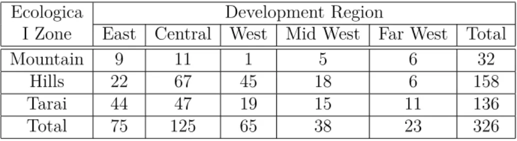
NLSS follows the World Bank’s Living Standards Measurement Survey (LSMS) methodology and uses a two-stage stratified sampling scheme. NLSS II enumerated 3,912 households from 326 Primary Sampling Units (PSU) of the country.

Stratification

The sampling design of the survey NLSS was two-stage stratified sampling. The to-tal sample size (3,912 households) were selected in two stages. The sample of 326 PSUs were selected from six strata using Probability Proportional to Size (PPS) sampling

(32)

with the number of households as a measure of size. Within each PSU, 12 households were selected by systematic sampling from the total number of households listed. The NLSS sample was allocated into six strata as follows: Mountains (384 households in 32 PSUs), Kathmandu valley urban area (408 households in 34 PSUs), Other Urban areas in the Hills (336 households in 28 PSUs), Rural Hills (1,152 households in 96 PSUs), Urban Tarai (408 households in 34 PSUs) and Rural Tarai (1,224 households in 102 PSUs). Table A.1 in Appendix presents the geographic distribution of the sampled PSU by regions and belts.

4.1.2

Health Status

Health status questionnaire is covered in Section 8. This section collected infor-mation on chronic and acute illnesses, uses of medical facilities, expenditures on them and health status. Health status questionnaire is asked for every individual that was covered in the survey.

The health status questionnaire has four options. For our purpose we make it bi-nary variable. We keep excellent health condition as 1 and other zero. So we have health status with excellent health condition 58.2 percentage. The survey data show that there are 60.35 percent male and 56.21 percent female have excellent health con-dition reported. Urban reported more excellent health status than rural area. Urban has 63.87 percent excellent health condition versus 56.01 percentage in rural area. By religion Hindu has 58.89 percentage excellent health status and non-hindu has 55.19 percentage excellent health status.

4.1.3

Covariates

We choose five relevant covariates which can influence health status from same NLSS survey for Integrated Multivariate Normal Approximation (IMNA) Logistic method. They are age, indigenous, sex, area and religion. We created binary variable indigenous as whether indigenous or not (Indigenous = 1, Non-indigenous = 0), religion as whether Hindu or not (Hindu = 1, Non-Hindu = 0), sex as whether male or female (Male = 1, Female = 0) and area as whether urban or not (Urban = 1, Rural = 0). For continuous covariate age we standardized it. We believe that health status could be affected by age of the individual. Older age and child age are more voulnerable than younger age. Indigenous are those who lived within the same territory for thousands of years for many many generations. We believe they could have different health status than other migrated people. Similarly, health status of urban and rural citizens could be different. Frequency tables for the covariates are shown in the Appendix (Tables A.3, A.4, A.5, A.6). Also the distribution of age (the continuous covariate) shown in Figure A.1 of the Appendix.

(33)

4.1.4

Quality of Data

To maintain the quality of data, a complete household listing operation was un-dertaken in each selected PSUs during March-May of 2002, about a year prior to the survey. Systematic sample selection of households was done in the central office. The field staff consists of supervisors, enumerators and data entry operators. Female in-terviewers were hired to interview female respondents for sensitive questions which are related to women such as their marriage and maternity history and family planning practices.

Data collection was carried out from April 2003 to April 2004 in an attempt to cover a complete cycle of agricultural activities, health related questionnaire and to capture seasonal variations in different variables. The process was completed in three phases. Data entry was done in the field. Separate data entry program with consistency check-ing was developed for this survey. There was consistency checkcheck-ing for each question-naire linked between sections. All errors and inconsistencies were solved in the field. Data were collected through out the year.

4.1.5

Questionnaire

The questionnaire that collect information about chronic illness of all household members in the survey is shown in Figure A.2 in Appendix.

4.2

Exact Method Output Analysis

As for the simulated samples we obtained from exact method by Metropolis Hast-ings sampler, diagnostics need to be performed to determine convergence and to obtain

random samples. The Geweke test output of samples for parametersβand δ2 _{is shown}

as follows.

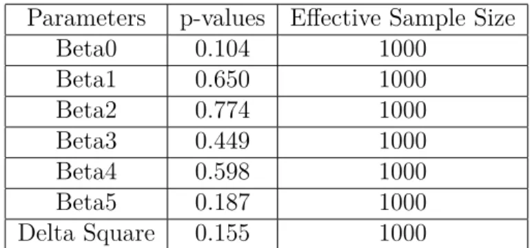
We simulated 11,000 iterations in total for Metropolis Hastings sampling. We have used 1,000 samples as a burn-in and we used every tenth iterate. After burn-in and thinning, we get the final 1,000 samples. The Geweke test for stationarity of the

parameters β and δ2 _{are shown below. The p-values are much higher than 0.05 and}

(34)

Parameters p-values Effective Sample Size Beta0 0.104 1000 Beta1 0.650 1000 Beta2 0.774 1000 Beta3 0.449 1000 Beta4 0.598 1000 Beta5 0.187 1000 Delta Square 0.155 1000

Table 4.1: Geweke results for parameters by exact method

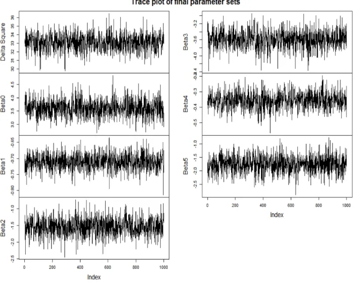
Figure 4.1 are the trace plots for all beta parameters and delta squared. There are 1,000 samples left as final samples. These trace plots show that samples are random and mixing well.

(35)

(36)

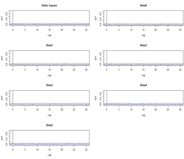
Figure 4.2 are autocorrelation plots for parameters beta and delta squared. These plots do not show any dependency among samples.

(37)

4.3

Result Comparison of IMNA and Exact Method

We compare the processing times of the IMNA method and exact method in order to find a faster computation. The total time for exact method is 17.46.18 minutes (1,066.18 seconds) for 1,000 samples while only 0.20.65 minutes for IMNA method with 1,000 samples, more than 50 times faster than the exact method. So it is obvious that integrated multivariate normal approximation (IMNA) method is much faster and equally reliable as exact method.

These are computation for 3,912 households in the survey. Suppose there are

1,000,000 households in our dataset. Then, assuming propotional allocation the to-tal time for respectively the exact method and IMNA method could be approximately 76 hours and 1.5 hours with 1,000 samples each. This will make a lot of difference in big data analysis.

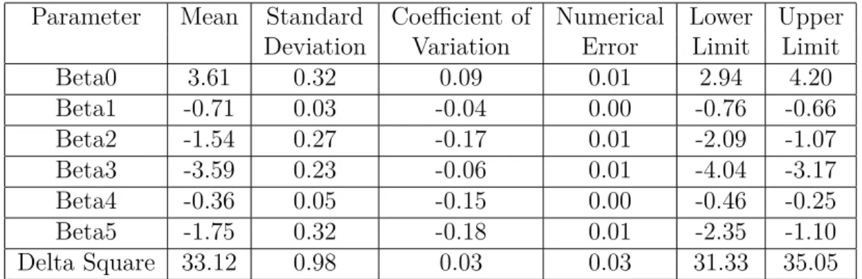
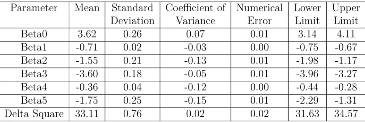
The estimates for parameters beta and delta square by exact and IMNA method are in Table 4.3 and Table 4.4. The mean of parameters and numerical error by the two methods are close. IMNA has slightly smaller standard deviations and coefficients of variation than exact method. Although the intervals are a bit shorter for IMNA than the exact method, our conclusions are basicly the same based on interval estimation. This suggests that inference for IMNA is reasonably close to the exact method.

Parameter Mean Standard Coefficient of Numerical Lower Upper

Deviation Variation Error Limit Limit

Beta0 3.61 0.32 0.09 0.01 2.94 4.20 Beta1 -0.71 0.03 -0.04 0.00 -0.76 -0.66 Beta2 -1.54 0.27 -0.17 0.01 -2.09 -1.07 Beta3 -3.59 0.23 -0.06 0.01 -4.04 -3.17 Beta4 -0.36 0.05 -0.15 0.00 -0.46 -0.25 Beta5 -1.75 0.32 -0.18 0.01 -2.35 -1.10 Delta Square 33.12 0.98 0.03 0.03 31.33 35.05

(38)

Parameter Mean Standard Coefficient of Numerical Lower Upper

Deviation Variance Error Limit Limit

Beta0 3.62 0.26 0.07 0.01 3.14 4.11 Beta1 -0.71 0.02 -0.03 0.00 -0.75 -0.67 Beta2 -1.55 0.21 -0.13 0.01 -1.98 -1.17 Beta3 -3.60 0.18 -0.05 0.01 -3.96 -3.27 Beta4 -0.36 0.04 -0.12 0.00 -0.44 -0.28 Beta5 -1.75 0.25 -0.15 0.01 -2.29 -1.31 Delta Square 33.11 0.76 0.02 0.02 31.63 34.57

(39)

Figure 4.3 is comparison of posterior means for proportions of excellent health status in each household (small area in our case) for IMNA and exact methods. This

plot is almost 45◦ _{straight line through the origin, which shows that posterior means}

for the proportions from IMNA method and exact method are close.

Figure 4.3: Posterior means for proportions of health status by exact and IMNA method

(40)

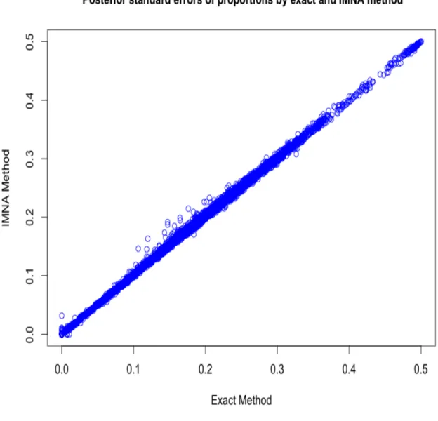
Figure 4.4 is comparison plot of posterior standard errors of proportions for IMNA

and exact method. Almost all points are on the 45◦ straight line through the origin,

while few households show slightly higher standard errors for IMNA method for stan-dard errors between 0.12 and 0.23. This plot shows that there is almost no difference in posterior standard errors of the proportions from IMNA and exact methods.

(41)

Linear Regression of Posterior Means of IMNA on Exact Method

We run linear regression on posterior means for the proportions of IMNA on exact method.

The standard error for residuals is 0.00457 with 3910 degrees of freedom. The p-value for F test is less than 2.2×10−16_{, and} _R2 _{= 0}_._{9997, suggesting a very good fit}

of linear regression. The t-test p-values for intercept and regressor are almost zero,

suggesting strong significance. The intercept value is around zero (0.0015274) with

very small standard error (0.0001140) and regressor estimate almost one (0.9987685)

with small standard error (0.0002836). This shows that the two methods are very much

close in their posterior means for the proportions.

Estimate Std. Error t value P r(>|t|)

(Intercept) 0.0015274 0.0001140 13.39 <2e−16 ***

output avg1 0.9987685 0.0002836 3521.22 <2e−16 ***

Table 4.4: Linear regression output for posterior means

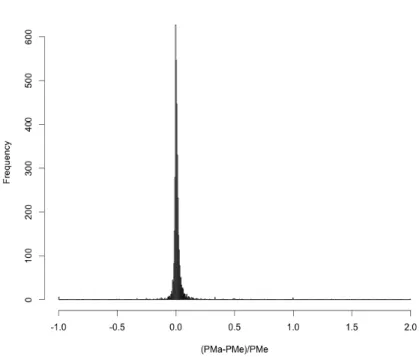
The histogram of difference between posterior mean for proportion estimation by IMNA and exact method scaled by exact method is shown in Figure 4.5. This histogram is centered around zero with small variation. This histogram also confirms that the results of IMNA method and exact method are very much similar.

(42)

PMa is posterior means by IMNA, PMe is posterior means by exact method Figure 4.5: Histogram of (PMa-PMe)/PMe

Linear Regression on Posterior Standard Deviations of IMNA and Exact Method

We also run linear regression on posterior standard errors for the proportions of IMNA on exact method.

The standard error for residuals is 0.00401 on 3910 degrees of freedom. The p-value for F test is p−value < 2.2×10−16_{, and} _R2 _{= 0}_._{9987, suggesting a very good fit}

of linear regression. The t-test p-values for intercept and regressor are almost zero,

suggesting strong significance. The intercept value is around zero (0.0015365) with

very small standard error (0.0001232) and regressor estimate almost one (1.0009586)

with small standard error (0.0005872). This shows that the two methods are very much

close in their posterior standard errors for the proportions.

Estimate Std. Error t value P r(>|t|)

(Intercept) 0.0015365 0.0001232 12.47 <2e−16 ***

output std1 1.0009586 0.0005872 1704.74 <2e−16 ***

Table 4.5: Linear regression output for posterior standard errors

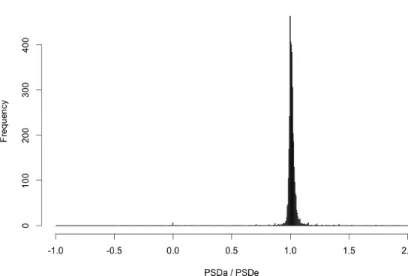
The histogram of ratio of posterior standard error for proportion estimation by IMNA and exact method is shown in Figure 4.6. This histogram is centered around

(43)

one with small variation. This histogram also confirms that the results of IMNA method and exact method are very much similar.

PSDa is posterior