Fernandes, F. D. S., Stasinakis, C. and Bardarova, V. (2018) Two-stage
DEA-Truncated Regression: Application in banking efficiency and
financial development.
Expert Systems with Applications
, 96, pp. 284-301.
(doi:
10.1016/j.eswa.2017.12.010
)
This is the author’s final accepted version.
There may be differences between this version and the published version.
You are advised to consult the publisher’s version if you wish to cite from
it.
http://eprints.gla.ac.uk/156248/
Deposited on: 22 January 2018
Enlighten – Research publications by members of the University of Glasgow http://eprints.gla.ac.uk
1
Two-stage DEA-Truncated Regression: Application in Banking Efficiency and
Financial Development
Filipa Da Silva Fernandesa Charalampos Stasinakisb*
Valeriya Bardarovac
aSchool of Economics, Finance and Accounting, Faculty of Business and Law, Coventry University, Priory Street, Coventry, United Kingdom, CV1 5FB. Email address: [email protected]
b Department of Accounting and Finance, Adam Smith Business School, University of Glasgow, University Avenue, West Quadrangle, Gilbert Scott Building, Glasgow, United Kingdom, G12 8QQ. Email address: [email protected] , Phone number: +44 (0) 141 330 7591- * Corresponding Author
c University of Edinburgh Business School, University of Edinburgh,29 Buccleuch Place, Edinburgh, United Kingdom, EH89JS. Email address: [email protected]
Abstract
This study evaluates the efficiency of peripheral European domestic banks and examines the effects of bank-risk determinants on their performance over 2007-2014. Data Envelopment Analysis is utilized on a Malmquist Productivity Index in order to calculate the bank efficiency scores. Next, a Double Bootstrapped Truncated Regression is applied to obtain bias-corrected scores and examine whether changes in the financial conditions affect differently banks’ efficiency levels. The analysis accounts for the sovereign debt crisis period and for different levels of financial development in the countries under study. Such an application in the respective European banking setting is unique. The proposed method also copes with common misspecification problems observed in regression models based on efficiency scores. The results have important policy implications for the Euro area, as they indicate the existence of a periphery efficiency meta-frontier. Liquidity and credit risk are found to negatively affect banks productivity, whereas capital and profit risk have a positive impact on their performance. The crisis period is found to augment these effects, while bank-risk variables affect more banks' efficiency when lower levels of financial development are observed.
2
1. Introduction
Data Envelopment Analysis (DEA) is a non-parametric linear programming technique, which extends the idea of estimating efficiency by comparing each Decision Making Units (DMUs) with an efficient production frontier (Farrell, 1957). As introduced by Charnes et al. (1978), DEA defines the set of best-practice observations for the DMUs under study and produces a convex production possibilities set by connecting the best-practice observations with a piecewise linear frontier. This principle is the basis of the traditional DEA and its applications are spread across different scientific disciplines (Serrano-Cinca et al., 2005; Lee, 2010; Chiang and Che, 2015; LaPlante and Paradi, 2015).
The banking sector plays a crucial role in the development of any financial system. Consequently, identifying ways to analyse the efficiency of banks has been in the centre of policy makers’, economists’, institutions’ and academics’ research. For that reason, the DEA literature on banking efficiency is voluminous. Nonetheless, it is characterised by different methodological approaches and mixed results. Most studies traditionally focus on US and European markets, as illustrated by the cornerstone survey work of Berger & Humphrey (1997). The scope in later years shifts primarily in the European setting. For example, Altunbas et al. (2001) analyse the efficiency of German banks in relation with their type of ownership types and they claim that there is no significant evidence to suggest that privately owned banks are more efficient than their mutual and public sector counterparts. Maudos and Pastor (2003) control for cost and profit efficiencies for the Spanish and Italian banks respectively and they note that most efficient and profitable institutions are able to better control costs. Chortareas et al. (2009) examine the case of Greece with several metrics of banks’ efficiency and they conclude that controlling for risk preferences is important in determining bank efficiency.
The above studies follow a single-country DEA approach. The rationale behind this choice is that the cross-country banking sector cannot be considered homogeneous due to national variations in legal tradition, regulatory frameworks, culture and religion (Berger, 2007). Lately, vast numbers of studies knuckle down to European comparative studies. This cross-country shift is driven mainly by two factors. Firstly, the introduction of the Single Market in the European Union over the nineties raised the expectations for higher financial integration and bank efficiency convergence within Europe (Bos and Schmiedel, 2007; Weill, 2009). Secondly and most importantly, the Global Financial and Eurozone sovereign debt crises demonstrated the need for a tighter banking sector union, especially in the Eurozone periphery (Casu et al., 2016).
3 One such example is the work of Casu et al. (2004) who evaluate the productivity changes in European banking between 1994 and 2000. Their results imply that productivity growth is brought through improvements in technological change, rather than technical efficiency. Altunbas et al. (2007) conclude that there is a clear relationship between capital, risk and efficiency, as European inefficient banks tend to hold more capital and take on less risk. Brissimis et al. (2008) evaluate the banking efficiency across newly acceded EU countries and they find that the banking sector reform and competition impact positively the bank efficiency, while capital and credit risk negatively effect bank performance. Finally, Casu and Girardone (2010) discuss how integration and efficiency convergence appears in EU banking markets. Their results indicate that there is a level of convergence towards a European efficiency average, but this pattern does not lead to efficiency improvements across all countries. Casu et al. (2016) recently evaluate the effect of the Eurozone crisis and observe a structural break in bank productivity growth in the Eurozone countries at the start of the crisis. This is particularly interesting, given that the Eurozone markets have small capital markets. In 2012, Greece, Ireland, Italy, Portugal and Spain (GIIPS) saw their stock market capitalisation to further reduce.1 During this period, banks faced liquidity shortages and higher
credit risk, which led to cuts of their lending conditions up to 47% for Small and Medium Enterprises (SMEs). Logically focusing on the periphery economies should provide further insight on what effect capital markets’ development has on banking efficiency. The intuition behind that is that banks and capital markets can be complementary to one another, as capital market development lowers the cost of bank equity capital. Consequently, this enables banks to raise the extra capital needed to take on riskier loans that they would otherwise reject (Vazquez and Federico, 2015). Other studies show that the sovereign debt crisis adversely affects the European stock markets and as a result, countries with poor credit market regulations and with larger pre-crisis account deficits (Giannonne
et al., 2011 and Grammatikos and Vermeulen, 2012). With this in mind, the European Commission (EC) initiatives and vision (BASEL III and Capital Market Union (CMU)) to allow capital markets’ development and deepen the banking integration seem especially relevant for fostering growth in the Eurozone periphery (Durusu-Ciftci et al., 2017).
From a methodological point of view, DEA continues to be very popular for practitioners as a technique for evaluating DMUs’ efficiency (Asosheh et al., 2010). Its application is easy and interpretable, while it is able to
4 project an efficient frontier formed by linear combinations connecting the set of ‘best-practice’ observations in the dataset. A DEA practitioner does not need to make assumptions about the distribution of inefficiency, while Fethi and Pasiouras (2010, p.190) suggest that DEA ‘does not require a particular functional form on the data in determining the most efficient banks’. Compared to other parametric techniques, DEA is also able to cope with small sample sizes and the application of categorical variables that are commonly used in country-specific panels of data (Brissimis et al., 2008; Fethi and Pasiouras, 2010). This is particularly important for banking datasets that are usually small in nature. In traditional statistical approaches (e.g. regression analysis), small sample size comes at a cost as the average DMU behaviour is of interest. On the other hand, DEA focuses on the performance of each DMU. Therefore, the number of DMUs in a DEA framework could be considered immaterial (see amongst others and Cook et al. (2014) and Tsolas and Charles (2015)). Finally, most parametric approaches introduce time trends to the data which lead to smoothing out the variation of the productivity changes.
Additionally, there is no consensus around the DEA orientation (Cook et al. 2014). Many researchers advocate the input-oriented approach assuming that bank managers impose control over inputs (e.g. expenses) rather than outputs (e.g. income) (Wu et al., 2006; Khodabakhshi et al., 2010; Tsolas and Charles, 2015). On the other hand, others believe it is more appropriate to answer how can output quantities be proportionally expanded without changing the underlying input quantities used over different time periods (see amongst others Grifell-Tatjé and Lovell (1997), Fethi and Pasiouras (2010) and Bassem (2014)). Although the literature is conflicting, many studies suggest that the choice of orientation has minimum effect upon the actual calculated scores. Therefore, the DEA orientation should not be a point of friction across researchers’ approaches.
Several studies on banking efficiency proceed to a two-stage approach, where efficiency scores are estimated in the first stage and then simply regressed on independent environmental variables (Wang et al., 2003; Beccalli et al., 2006; Sun and Chang, 2011). This approach is problematic for the following reasons. Firstly, the estimated distances from the DEA frontier can be underestimated when optimal DMUs are excluded from the sample (sample bias). Secondly, traditionally DEA estimates (not incorporating Malmquist index approaches) introduce boundary inefficiencies in the OLS method. Finally, efficiency scores suffer from high serial correlation, which impedes their statistical interpretability and valid estimation. All these disadvantages are clearly explained by the influential work of Simar and Wilson (2007). The authors introduce a Double-Bootstrapped Truncated Regression (DBTR) framework, which copes with the above issues and provides bias-corrected efficiency scores. The benefits of this
5 approach are well-documented in the respective banking literature (see amongst others Feng and Serletis (2010), Assaf et al. (2011), Chortareas et al. (2013), Wanke and Barros (2014), Wanke et al. (2016)).
The above background positions this work clearly in the respective literature and clarify its motivation. Firstly, DEA efficiency scores based on a Malmquist Productivity Index (MPI) are calculated on a cross-country level, namely the peripheral economies of GIIPS. This approach, although not the only available for efficiency scores’ calculation, is common in the respective literature (see amongst others Färe et al. (1994), Casu et al. (2004), Tortosa-Ausina et al., (2008) and Kevork et al. (2017)). In our case, efficiency is evaluated based on the five metrics derived from the ‘enhanced decomposition’ proposed by Färe et al. (1994). Secondly, a DBTR framework is adopted in order to reconstruct the initial DEA estimates into bias-corrected ones which are optimized for the second-stage regression.
This study is offering several innovations in terms of the methodological approach undertaken. We further validate the success of the MPI’s ‘enhanced decomposition’ and Simar’s and Wilson’s (2007) approach. In particular, we provide a unique setting to calculate different bank efficiency metrics and evaluate the effects of bank-risk variables and financial development on them through regression specifications. These are based on the second algorithm proposed by Simar and Wilson (2007). The selection of this algorithm is crucial, as in two-stage DEA regressions the covariates in the second-step can be highly correlated with the covariates in the first-step. This would clearly offer a rejection of the initial assumption of independence between them and the errors (Fethi and Pasiouras, 2010). Applying these regressions allow us to assess in a robust econometric way, whether changes in the financial conditions of peripheral European banks in and out-of-the crisis affect differently their efficiency, taking into account the level of financial development in the respective countries. Specifically, we are interested in identifying which (if any) bank-level risk characteristics are important factors in shaping banks’ operations. In order to achieve that, we construct a balanced panel over the period of 2007-2014 with variables that traditionally are considered determinants of banks’ behaviour. We find that higher levels of liquidity risk and credit risk exert a negative effect on banks’ efficiency levels, whereas capital risk and profit risk have a positive one. Additionally, bank risk variables have a more negative impact during the crisis than outside of the crisis period. Finally, when we consider the indirect role of financial development, it is clear that bank-risk variables exert a higher impact on banks’ efficiency for lower levels of financial development during the crisis. These are important and innovative results, when
6 discussing banking efficiency in the GIIPS and integration of their financial institutions in the European single market.
This study also claims that the MPI efficiency metrics can be considered as early warning indicators of financial instability and potentially used as macroeconomic tools to evaluate the financial system and its capital development. This is a novel notion in the respective literature, which is supported the evidence of a domestic bank efficiency meta-frontier within the peripheral economies that this study brings forward. A meta-frontier in a DEA framework is an efficiency frontier that covers the performance of all DMUs operating in different regions under different technologies. Although the methodological scope of this study is not to perform meta-frontier analysis per se, the identification of similar performances of banks across different countries is very important for practitioners and policy makers that are interested to further investigate this issue within the European banking environment(Bos and Schmiedel, 2007).
Overall, the contribution of this study to the relevant banking literature is multi-fold. Firstly, the empirical evidence provides a precise and econometrically robust DEA analysis for the Eurozone periphery, extending the previously mentioned trend to cross-country comparative studies. Casu et al. (2016) present a relevant analysis, but the authors do not apply the principles of the truncated regression and exclude Ireland from their analysis. As such, a full picture on the peripheral economy is not provided and at the same time their DEA results might be biased, especially during the calculation of the meta-frontier. Secondly, to the best of our knowledge there is no other paper connecting the effects of financial development on the Eurozone’s periphery banks. Thirdly, very little research is available on the impact of the sovereign debt crisis on banks’ activities. This is confirmed by Lenarčič et al. (2016), who clearly state that the effects of sovereign risk to bank balance sheets remain unexplored, despite the extensive reforms in bank regulation over the last years. This work goes towards bridging this clear gap in the literature. Finally, the following studies seem relevant to the context under study. Popov and Van Horen (2013) identify a direct link between deterioration in a bank’s sovereign debt portfolio and bank lending in the loan market. Bedendo and Colla, (2015) explore the relation between a country’s sovereign debt quality and the credit risk of domestic non-financial firms. Recently, Ferrando et al. (2015) explore the effect of the sovereign debt crisis on SMEs access to banks finance. However, none of the three clearly focuses on the role of the sovereign debt crisis on banks productivity.
7 The remainder of this paper is structured as follows. Section 2 describes the two-stage methodology adopted in this study, namely the DEA-MPI and the DBTR, while section 3 presents the respective dataset. Section 4 summarizes all the empirical results obtained. Finally, section 5 provides some concluding remarks.
2. Methodology
This section describes the methodological approach undertaken in order to obtain unbiased bank efficiency scores and evaluate the effects of bank-specific variables on them. Initially, we motivate the selected variables and the orientation of our model. Then, the DEA based on Malmquist Productivity Index (DEA-MPI) is presented. Finally, the Double-Bootstrapped Truncated Regression (DBTR) is explained along with the selected regression specifications.
2.1 Variables and orientation selection
Another issue that needs to be clarified before implementing DEA is the balance of the number of inputs and outputs. Although Cook et al. (2014) suggest that the number of evaluated DMUs may be immaterial in cases, a parsimonious solution can be reached only by restricting the input-output set. For that reason, we follow the well-accepted ‘rule of thumb’ proposed by Cooper et al. (2007), based on which the number of DMUs must be higher than three times the sum of inputs and outputs. The authors claim that if this rule does not hold, then large number of DMUs might be found efficient. However, the lack of degrees of freedom is likely to make the efficiency discrimination questionable. For that reason, in our case two inputs and one output are selected to measure productivity change.
The nature of these three variables falls within the debate of DEA vector selection. This debate is not only econometrical (number of inputs and outputs), but it is also theoretical within a banking context. Early studies address banking efficiency through the intermediation and production approaches.Berger and Humphrey (1997) claim, though, that neither of the two methods captures appropriately the role of banks as financial intermediaries and transaction processing services’ suppliers. For that reason, in this study the profit-based DEA is applied, which uses revenues as outputs and costs as inputs. This allow us to form a technology set based on spending and earnings of the observed DMUs. Such an approach is more meaningful for a bank, when its underlying behavioural objective is the profit maximization (Sahoo et al., 2014). Profit-based input/output selection can lead to efficiency scores
8 capturing better the decision-making diversity across financial institutions, when those are responding to their competitive environment (see amongst others Maudos et al. (2002), Drake et al., (2006) and Sahoo et al., (2014)). The traditional economic factors driving productivity are land, labour and capital. Operating expenses can be thought as a proxy for land, labour wages, physical capital expenses and provisions for doubtful loans. Interest expenses can also be a proxy for the capital provided by the banks’ stakeholders or by its depositors. For that reason, they are both selected as inputs for our analysis. The output variable is the total income calculated as the sum of interest and non-interest income2.
Finally, as mentioned earlier, there is no consensus regarding the DEA orientation selection (Cook et al., 2014). Nonetheless, every practitioner needs to make a ‘judgement call’ when it comes to implementing DEA. In our case, we implement an output-oriented DEA. In that scenario, the efficiency scores show the possible proportional increases in the output levels, while the inputs proportions remain unchanged. Following studies related to the ‘social control’ of banks (Ataullah et al., 2004), we postulate that banking is output-oriented in nature, as bank managers are expected to have more flexibility with the bank’s outputs rather than its inputs, especially in countries with tightening financial and economic environment (Casu et al., 2004; Ataullah and Le,2006; LaPlante and Paradi, 2015).
2.2 First stage: DEA-MPI
The first stage of this study utilizes a DEA approach based on the MPI to investigate how productivity of each bank changes through time. This is done by following an output-oriented DEA approach described by Färe et al., (1994). Let 𝑥𝑡 ∈ 𝑅
+𝑁 𝑎𝑛𝑑 𝑦𝑡 ∈ 𝑅+𝑀 the selected input and output variables (for N*1 input and M*1 output vectors) and n
the total number of banks, then the production set3𝑃𝑡 in time 𝑡 can be expressed as:
𝑃𝑡 = {(𝑥𝑡, 𝑦𝑡): 𝑥𝑡 𝑐𝑎𝑛 𝑝𝑟𝑜𝑑𝑢𝑐𝑒 𝑦𝑡} (1)
The production frontier with the output-oriented distance function under the assumption of Constant Returns to Scale (CRS) can be defined as:
2 Interest expense is more accurate than the total amount of deposits as not all deposits carry the same interest expense. DEA is not
efficient in dealing with negative values. Hence, results for the banks whose non-interest income is negative will be questionable Therefore, the total income approach is preferred as the output vector.
3The production set is also commonly referred to as production frontier/technology (see amongst others Färe et al., (1994) and Simar and Wilson (2007)).
9 𝐷0𝑡(𝑥
𝑗𝑡, 𝑦𝑗𝑡) = min {𝜑 | (𝑥𝑗𝑡, 𝑦𝑗𝑡/𝜑) ∈ 𝑃𝑡}, 𝑗 = 1,2 … 𝑛 (2)
In equation (2), the ‘0’ subscript denotes the output orientation of the model. The distance aims to identify the reciprocal of the greatest proportional increase in output, given the input but also keeping the output feasible. In other words, it defines the technology of bank 𝑗 at time 𝑡 relative to the output technical efficiency at time 𝑡 (Färe
et al., 1994). Here, the technical efficiency is estimated relative to the contemporaneous technology as
𝐷0𝑡(𝑋
𝑗𝑡, 𝑌𝑗𝑡) ≤ 1. Only when the unit 𝑗 is on the production frontier (i.e. technically efficient), can the equation be
expressed in the form 𝐷0𝑡(𝑋𝑗𝑡, 𝑌𝑗𝑡) = 1. Alternatively, 𝐷0𝑡(𝑋𝑗𝑡, 𝑌𝑗𝑡) < 1 means that the unit below the frontier is
technically inefficient. To define the MPI, a specification of distance functions with respect to two different time periods is needed. At time 𝑡, the efficiency of unit 𝑗 relative to the technology at time 𝑡 + 1 is expressed by:
𝐷0𝑡 (𝑥
𝑗𝑡+1, 𝑦𝑗𝑡+1) = min {𝜑| (𝑥𝑗𝑡+1, 𝑦𝑗𝑡+1/𝜑) ∈ 𝑃𝑡}, }, 𝑗 = 1,2 … 𝑛 (3)
This distance measures the maximum proportional change in outputs required to make (𝑥𝑗𝑡+1, 𝑦𝑗𝑡+1) feasible in relation to technology at time t. Distance functions are computed by employing a DEA linear programming methodology. The CRS output-oriented DEA problem is defined as below:
𝐷0𝑡(𝑥 𝑗𝑡, 𝑦𝑗𝑡)
−1
= max 𝜑𝑗 𝑠. 𝑡. {−𝜑𝑗𝑦𝑗𝑡+ 𝑌
𝑡 𝜆 ≥ 0, 𝑥𝑗𝑡− 𝑋𝑡𝜆 ≥ 0, 𝜆 ≥ 0} (4)
Where 𝑌𝑡and 𝑋𝑡represent the vector of outputs and inputs respectively and 𝜆 signifies the weight vector (a weight is assigned to each unit within the reference ‘peer’ group, which is compared to any particular observation in order to determine the distance to the efficient frontier). Caves et al. (1982) defined MPI (M) at two consecutive time periods (t, s) as: { 𝑀 𝑡(𝑥 𝑗𝑡+1 , 𝑦𝑗𝑡+1, 𝑥𝑗𝑡, 𝑦𝑗𝑡) = 𝐷0𝑡(𝑥𝑗𝑡+1, 𝑦𝑗𝑡+1)/𝐷0𝑡(𝑥𝑗𝑡, 𝑦𝑗𝑡) 𝑀𝑡+1(𝑥 𝑗𝑡+1 , 𝑦𝑗𝑡+1, 𝑥𝑗𝑡, 𝑦𝑗𝑡) = 𝐷0𝑡+1(𝑥𝑗𝑡+1, 𝑦𝑗𝑡+1)/𝐷0𝑡+1(𝑥𝑗𝑡, 𝑦𝑗𝑡) (5)
To avoid the use of an arbitrary benchmark, the two continuous MPIs are combined into one by estimating its geometric mean, which provides the calculation of the Total Factor Productivity Change (TFPCH):
𝑀0(𝑥𝑗𝑡+1 , 𝑦𝑗𝑡+1, 𝑥𝑗𝑡, 𝑦𝑗𝑡) = 𝑇𝐹𝑃𝐶𝐻 = {𝐷0 𝑡+1(𝑥 𝑗 𝑡+1,𝑦 𝑗𝑡+1) 𝐷0𝑡 (𝑥𝑗𝑡,𝑦𝑗𝑡) } ∗ [ 𝐷0𝑡(𝑥𝑗𝑡+1,𝑦𝑗𝑡+1) 𝐷0𝑡+1 (𝑥𝑗𝑡+1,𝑦𝑗𝑡+1)∗ 𝐷0𝑡(𝑥𝑗𝑡,𝑦𝑗𝑡) 𝐷0𝑡+1 (𝑥𝑗𝑡,𝑦𝑗𝑡)] 1 2 = {𝐸𝐹𝐹𝐶𝐻} ∗ 𝑇𝐸𝐶𝐻𝐶𝐻 (6)
When TFPCH >1 (<1), it is implied that there is an increase (decrease) in productivity, while TFPCH=1 refers to cases where productivity is deemed unchanged. From equation (6), it is also shown that TFPCH is decomposed into the Efficiency Change (EFFCH) and Technology Change (TECHCH) sub-indices as explained by Färe et al.
10 (1994). The EFFCH ratio measures change in technical efficiency of a DMU relative to the best practice frontier. This shows whether unit 𝑗 moves towards or away from the production frontier over the period from 𝑡 to 𝑡 + 1. A firm is deemed to be technically efficient if it is impossible to increase output without altering input usage. Specifically, efficiency is measured as the distance between the point the firm lies in the input–output space and the production frontier (technology) that envelops the data. The Technological Change (TECHCH) component is due to the variation of the production frontier between two periods and hence, exerts improvement or deterioration of the unit’s technology from 𝑡 to 𝑡 + 1. The EFFCH is further decomposed into improvements in management practices or movements toward an optimal size. As suggested by Färe et al. (1994), the first refers to a measure of Pure Technical Efficiency Change (PECH), while the latter to a measure of Scale Efficiency Change (SECH):
𝑃𝐸𝐶𝐻𝑡,𝑡+1=𝐷𝑜,𝑣𝑡+1(𝑥𝑗𝑡+1,𝑦𝑗𝑡+1)
𝐷𝑜,𝑣𝑡 (𝑥𝑗𝑡,𝑦𝑗𝑡) , 𝑆𝐸𝐶𝐻
𝑡,𝑡+1 = 𝐷𝑜,𝑐𝑡+1(𝑥𝑗𝑡+1,𝑦𝑗𝑡+1)∗𝐷𝑜,𝑣𝑡 (𝑥𝑗𝑡,𝑦𝑗𝑡)
𝐷𝑜,𝑐𝑡 (𝑥𝑗𝑡,𝑦𝑗𝑡)∗𝐷𝑜,𝑣𝑡+1(𝑥𝑗𝑡+1,𝑦𝑗𝑡+1)=>𝐸𝐹𝐹𝐶𝐻 = 𝑃𝐸𝐶𝐻 𝑥 𝑆𝐸𝐶𝐻 (7)
Here it should be noted that PECH is calculated relative to Variable Returns to Scale (VRS) technology, while the component of SECH is measured as the deviations between the VRS and CRS technologies. Therefore, the subscripts “o,v” and “o,c” specify VRS and CRS technologies applied respectively for this ‘enhanced decomposition’ (Casu et al., 2004). The adoption of CRS or VRS technology from an economic perspective alters the envelopment surface. CRS technology assumes that the output(s) will change proportionally to the change observed in the inputs, while VRS technology encompasses both increasing and decreasing returns to scale. Intuitively, VRS might seem more realistic, since arguing in favour of CRS means that banks are assumed to operate at an optimal scale (Fethi and Pasiouras, 2010). On the other hand, VRS technology solves the same problem of CRS by adding an extra constraint in the linear programming process (increasing computation needs), namely that the sum of λ’s is equal to unity. Many researchers suggest caution when adopting VRS for several reasons. For example, the model orientation becomes important, unlike the CRS case. In that sense, MPI applications seem more compatible with CRS, while the weight restriction can lead DMUs to operate with over- or under-fitted returns to scale (Soteriou and Zenios, 1999). Additionally, differences in banks’ size under VRS can lead to lead to overestimating large banks’ efficiencies (Berg et al., 1991; Noulas, 1997). Finally, Coelli et al. (2005, p. 80) suggest that the TFPCH measure remains practically the same in output-oriented MPI approaches like ours. Consequently, imposing importance to the orientation of the model through VRS seems unnecessary. For that reason, we opted to
11 calculate the main components (TFPCH, EFFCH and TECHCH) with CRS technology and apply VRS only to the enhanced decomposition (PECH, SECH)4.
The non-parametric Malmquist index does not require the profit maximisation or the cost minimisation assumption. If the practitioner is using panel data, MPI allows the decomposition of productivity changes into two components (technical efficiency change or catching up to the frontier, and technological change or changes in the best practice). Moreover, DEA-MPI is able to derive the efficiency estimates, isolating DMUs’ efforts to catch up to the frontier (i.e., changes in technical efficiency - EFFCH) from shifts in the frontier (i.e., technological change - TECHCH). This is particularly interesting in cases of bank efficiency studies, because the production frontier can shift upward or downward over time due to market structure (such as increased competition), innovation (i.e., technical progress), changes in regulatory policies (such as financial liberalisation), and severe financial disruptions and shocks (e.g., financial crises). This explains the extensive application of TFPCH in this strand of the literature (see amongst others Casu et al. (2004), Portela and Thanasoulis (2010), Duygun et al. (2016), Casu et al. (2016)).
2.3 Second stage: DBTR
For the second-stage of our analysis, we are motivated by the bootstrapping techniques on MPIs proposed by Simar and Wilson (1999). They propose a bootstrap estimation procedure for obtaining confidence intervals for input-oriented indices Malmquist indices of productivity and their decompositions. In our case, we are interested for output-oriented MPIs that are interacted with environmental variables (two-stage approach). For that reason, we follow the influential work of Simar and Wilson (2007) to calculated bias-corrected scores. Specifically, Simar’s and Wilson’s (2007) algorithm two of left truncation is applied for this purpose. The bias-corrected efficiency scores derived from the algorithm are then regressed on the set of environmental variables.
In general, the problem is explained by a probability density function 𝑓(𝑥𝑗𝑡, 𝑦𝑗𝑡, 𝑧𝑗𝑡), where 𝑧𝑗𝑡 the environmental variables each bank j is facing. The main assumption is that the original MPI efficiency score is given by
( , ) 1
t
j zj
j can be translated into the following regression specification
j ztj
j 1 (8)
4Here, it should be noted that all productivity scores are obtained from the software DEAP v2.1 developed by Coelli (1996), while the cross-section technology is applied.
12 Where ψ a smooth continuous function, 𝑧𝑗𝑡 a vector of the environmental variables, a vector of parameters estimated by maximum likelihood and
j 2) a continuous iid random variable independent of 𝑧𝑗𝑡.The steps of algorithm are presented below:
Step 1: Using the original data in 𝑃𝑡, compute the
j
Step 2: Apply maximum likelihood to obtain the estimates
,2 of ,2in the truncated regression of jon ztjfor the observations where j 1.
Step 3: Loop over steps 3.1-3.4 1000 times to extract n sets of bootstrap estimates
* 10001
j jL L
B
:
Step 3.1: Draw
j 2)for each j=1,..,n with truncating left at (1ztj). Step 3.2: Again compute the
*j ztj
jfor each j=1,..,n.Step 3.3: Set x*jt xtj and y*jt ytj
j / *jfor each j=1,..,n.Step 3.4: Calculate the
*j based on the new production setP*tobtained by all *t, *tj j
x y
Step 4: For each j=1,..,n.compute the bias-corrected jusing the Bjand the original j.
Step 5: Apply the maximum likelihood method to estimate the truncated regression of j on ztjyielding ,
.
Step 6: Loop over steps 6.1-6.3 1000 times to obtain a set of bootstrap estimates
1000 * * 1 , j L L B :
Step 6.1: For each j=1,..,n draw j )for each j=1,..,n with truncating left at (1ztj
). Step 6.2: Again compute the
**j ztj
jfor each j=1,..,n.Step 6.3: Apply the maximum likelihood method to estimate the truncated regression of
**j on ztjyielding*,*.
Step 7: Use , and Bjto construct estimated confidence intervals for each element of .
The end of this procedure generates a set of bias-corrected estimates of efficiency estimates j Effj5, which
consequently are applied as the final dependent variable in equation (8). For more mathematical details regarding this process the interested reader should refer to Simar and Wilson (2007). Finally, we should note that the FEAR package in R platform has been applied for the estimation of the DBTR (Wilson, 2008)6.
5The repetition of the process provides a solid approximation of the true sampling distribution. 2000 bootstrap interactions are performed and the
95-percent confidence intervals are constructed. Simar and Wilson (1999) provide the estimation of the smoothing bandwidth parameter as
1/6
(0.8* )
h DMU . The scope of this paper is the application of the DBTR in order to evaluate how the bank-risk variables and financial development affect banks’ efficiency. From the DBTR we obtain bank specific bias-corrected estimates and confidence intervals for all banks of all countries and years. These are not presented for the shake of space and are available upon request.
6 More specifically, the routines of boot.sw98, rnorm.trunc and treg. Alternatively, the same results can be obtained by the simarwilson routine from STATA software.
13 At this stage, several issues need to be pointed out in order to clarify the DBTR process. Firstly, the main argument in favour of Simar’s and Wilson’s (2007) work derives from the way efficiency scores are used. As the original efficiency scores are not directly observed and the two-stage procedure is affected by explanatory variables not used in the first-stage, it must be accepted that the error terms will be serially correlated to the explanatory variables. This ‘correlation arises in finite samples from the fact that perturbations of observations lying on the estimate frontier will in many, and perhaps all, cases cause changes in efficiencies estimated for other observations.’ (see Simar and Wilson (2007, p.33). Secondly, algorithm two is preferred over algorithm one. Simar and Wilson (2007) explain that the latter aims at improving inference, but it does not take under consideration the bias term (
( j) ( j) j
BIAS E ). Essentially, steps one and two of algorithm two are the same in algorithm one, but steps three and four employ an extra parametric bootstrap in order to produce estimates improved in terms of statistical significance and bias. Additionally, the authors conclude that this improvement comes at a low computational cost compared to algorithm one.
Thirdly, we mention in the introduction section that several similar studies calculate the efficiency scores and then without further consideration regress them with environmental variables. This is done usually with Tobit, simple OLS, GMM or GLS censored regressions. This is based on the fact that efficiency scores are bounded between zero and unity, therefore it is expected that the estimates will be biased unless censored. The crucial difference, though, is that from a truncated normal distribution the errors that fall below (1 t )
j
z
are not observed, unlike in censored models like the Tobit one. Afonso and St. Aubyn (2011) and Wanke and Barros (2017) suggest that in two-stage approaches employing small size datasets there is high probability for downward bias pushing many efficiency scores to zero. Based on the above, the left-truncated approach (bounding the unbounded MPI scores above unity) is a ‘safer’ one econometrically speaking. Finally, given that the cost input variables are considered endogenous (Lensink and Meesters, 2014), the utilization of bias-corrected estimates in a stochastic setting provides extra safety against the traditional endogeneity issues observed in regression specifications incorporating firm-level data (Van Biesebroeck, 2008).
14 2.3.1 DBTR specifications
By applying the DBTR this study aims to investigate the extent to which bank-specific characteristics have an impact on domestic banks efficiency at the periphery of the Euro area. Using the unbiased efficiency estimates and following previous literature on bank efficiency (Athanasoglou et al., 2008; Brissimis et al., 2008), we form the following baseline DBTR specification:
𝐸𝑓𝑓𝑗𝑡= 𝑐 + 𝑎′𝑋′𝑗𝑡+ 𝛽′𝑌′𝑗𝑡+ 𝜀′𝑗𝑡 (9)
Where 𝐸𝑓𝑓𝑖𝑡is the bootstrapped bias-corrected efficiency scores of a bank j at time t, c is a constant term, 𝑋′𝑗𝑡
comprises a vector of bank-specific financial variables assumed to capture the impact of financial risk on the level of bank efficiency, 𝑌′𝑗𝑡 is a vector of firm-specific and macroeconomic control variables and 𝜀𝑗𝑡 is the error term which includes the unobserved bank-specific effect and the idiosyncratic error.
To capture the role of risk in the second stage regressions, we differentiate between four different types of risk, namely capital, liquidity, profit and credit risk. The selection of these variables (vector 𝑋′) follow the CAMEL-based framework as in Doumpos et al. (2017)7. Capital risk (CapitalR) is defined as the ratio of equity to total assets, to measure banks’ capital strength. Higher levels of capital (lower capital risk) are associated with a safety net for banks as capital refers to the quantity of funds available to support their business (see Athanasoglou et al., 2008). Hence, it would be expected that more efficient banks are more capitalised, using less leverage, and have lower costs of bankruptcy and as a result have a lower need for external funding. Liquidity risk (LiquidityR) is defined as the ratio of total loans over total assets. If banks are not able to liquidate some of their assets or raise funds from new external sources at reasonable costs, they might be unable to meet their financial obligations (Casu
et al., 2016). Thus, banks with higher liquidity risk are expected to experience lower efficiency levels. The key profitability risk ratio (ProfitR) is defined as the ratio of net income over total assets and it capture banks’ levels of profitability. We hypothesise that higher levels of profits may increase banks’ efficiency, as higher profits lead banks to generate returns on their assets of portfolio (Sufian, 2014). Finally, credit risk is measured as the ratio of loan-loss provisions to loans. Higher levels of credit risk are normally associated with lower levels of profitability
7 According to Poghosyan and Čihák (2009), the CAMEL variables (where CAMEL stands for “Capital, Asset quality, Management,
Earnings, and Liquidity”) should be able to capture distress signals of banks. In our case, we follow these principles but we do not include expenses management ratios (i.e. cost to income), because these variables are used in the profit-oriented DEA of the first stage of our analysis.
15 (Brissimis, et al. 2008). Hence, a negative relationship between credit risk and efficiency levels of banks is expected.
The control variables (vector 𝑌′) are chosen based on the existing empirical literature on bank efficiency. To control for the extent of economies of scale, we add Size measured as the logarithm of banks’ real total assets. There is a consensus that larger size may decrease the costs of gathering and processing information (Pasiouras and Kosmidou, 2008). Hence, we expect a positive relation between size and efficiency. Furthermore, the real GDP growth (GDPg) is introduced to control for the macroeconomic environment and demand factors. It is expected that it will be positively associated with banks’ efficiency levels. Finally, our specifications account for the effects of inflation. The relation between bank efficiency and inflation is not clear. If inflation is anticipated (not anticipated) could mean that banks are able (not able) to adjust their interest rates and as a consequence raise (decrease) revenues at a faster pace than costs (Perry, 1992). Given the above motivation for our baseline model, we go further to investigate the extent to which, banks efficiency levels differ in the sovereign debt crisis years compared to more tranquil periods. To do so, a financial crisis dummy (Crisis) is initially included as below:
𝐸𝑓𝑓𝑗𝑡 = 𝑐 + 𝑎′𝑋′
𝑗𝑡+ 𝐶𝑟𝑖𝑠𝑖𝑠𝑗𝑡+ 𝛽′𝑌′𝑗𝑡+ 𝜀′𝑗𝑡 (10) Crisis takes the value of one for the period between 2010 and 2012, and zero otherwise. Equation (10) aims to capture the marginal effect of the crisis on banks’ efficiency, assuming everything else constant (direct effect). The next step is to evaluate whether the sovereign debt crisis may also have an indirect effect by magnifying the impact of the internal factors on domestic banks efficiency levels. To this end, the equation below includes interaction terms between the three different types of risk and the crisis dummy:
𝐸𝑓𝑓𝑗𝑡= 𝑐 + 𝑎′𝑋′
𝑗𝑡∗ 𝐶𝑟𝑖𝑠𝑖𝑠𝑗𝑡+ 𝜕′𝑋′𝑗𝑡∗ (1 − 𝐶𝑟𝑖𝑠𝑖𝑠𝑗𝑡) + 𝛽′𝑌′𝑗𝑡+ 𝜀′𝑗𝑡 (11)
Comparing the coefficients on the two interaction terms allows us to assess whether changes in bank specific-characteristics have a different impact on banks’ efficiency. This test is motivated by the 2010-2012 events, which led periphery banks of the Euro area to tighten their credit standards as sovereign risk increased and worsened bank’s balance sheets (Acharya et al., 2016).
The final analysis of this study tests whether changes in the different types of risks in- and out- of the crisis period affect differently the domestic banks’ efficiency, taking into account countries’ level of capital market development (FD). We use the degree of stock market capitalisation as a sorting device. Stock market capitalisation to GDP is an efficient measure of stock market size. Larger stock markets are considered to have higher mobility of capital
16 and less volatility of risk (Demirguc-Kunt and Levine, 1996). The countries in our sample are classified into more and less financially developed based on the average stock market capitalisation to GDP. Hence, countries above (below) the mean of stock market capitalisation are more (less) financially developed. 8 We interact the vector of
risk measures with a FD and (1-FD) terms respectively. Thus, the final DBTR regression is specified as follows:
𝐸𝑓𝑓𝑗𝑡= 𝑐 + 𝑎′𝑋′
𝑗𝑡∗ 𝐶𝑟𝑖𝑠𝑖𝑠𝑗𝑡∗ 𝐹𝐷𝑡+ 𝜕′𝑋′𝑗𝑡∗ (1 − 𝐶𝑟𝑖𝑠𝑖𝑠𝑗𝑡) ∗ 𝐹𝐷𝑡+ 𝜔𝑋′𝑗𝑡∗ 𝐶𝑟𝑖𝑠𝑖𝑠𝑗𝑡∗ (1 − 𝐹𝐷𝑡) + 𝜏′𝑋′
𝑗𝑡∗ (1 − 𝐶𝑟𝑖𝑠𝑖𝑠𝑗𝑡) ∗ (1 − 𝐹𝐷𝑡) + 𝛽′𝑌′𝑗𝑡+ 𝜀′𝑗𝑡 (12)
We hypothesise that the Euro area larger bank balance sheets and smaller capital markets are directly related phenomena. Considering that periphery banks interrupted lines of credit due to liquidity problems during the crisis and that their access to capital markets is low, we expect that bank-specific risk variables exert a higher (lower) impact on bank efficiency during the crisis for lower (higher) levels of financial development.
3. Data and descriptive statistics
The data for this study is obtained from different sources including the Bankscope database, World Bank and World Development Indicators (WDI). The data cover 64 banks in five Euro area periphery economies- Greece, Ireland, Italy, Portugal and Spain-during the 2007-2014 period. To construct our balanced bank-level dataset (DEA input/outputs – vectors X and Y) , we use the 2015 version of the Bankscope database.9 The dataset includes only domestic commercial banks. As Pasiouras and Kosmidou (2007) suggest, selection of only commercial banks allow us to avoid issues of comparison between different type of banks such as savings, investment and cooperative banks. Following the standard procedure (Guariglia et al., 2015), we use only consolidated figures to the extent possible to avoid double counting. To control for potential outliers, observations below the 0.5 percentile and above the 99.5 percentile are removed. Annual data on GDP growth and inflation come from the World Bank Database.
8 We have also employed different proxies for FD, for example, the level of concentration and the ratio of stock market capitalisation
to total assets of the deposit money banks. Results remain robust to the ones presented for the FD proxy. Results are available upon request.
9 The number of banks per country are as follows: Greece (5), Ireland (4), Italy (37), Portugal (6) and Spain (12). The collected data
are from 2006-2014, but we can only report efficiency scores from 2007 as one year is lost for the calculation of the original MPI scores. Finally, using Bankscope has two main advantages. First, it accounts for about 90% of total assets in each country. Second, all information is provided in standardised format, which allows us to compare information within a country as well as across countries.
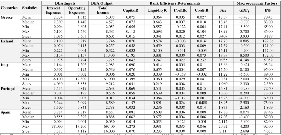
17 Table 1 below presents the summary statistics for all the variables, which are implemented in the first and second stage models. <insert Table 1>
Table 1 provides the summary statistics for the DEA inputs and all bank efficiency determinants used in this analysis. We find that domestic banks in Greece and Spain present the highest average levels of interest expenses and operating expenses when compared with their periphery counterparts. Over the sample period, Italian and Spanish banks present higher capital and liquidity risk ratios. Greek banks display the largest average values of credit risk whereas Ireland banks show a negative average profitability ratio. Overall, these preliminary results shed light on the idea that local periphery banks were largely exposed to their own countries sovereign debt leading to a deterioration of their assets quality, and therefore increasing their risk of default. This is consistent with Acharya and Steffen (2015) according to which domestic periphery banks shift from safer to riskier government bond by placing a bet on their own survival. More specifically, Acharya et al. (2016) claim that during the sovereign debt crisis, domestic periphery banks increased their exposure to government bonds transferring their risk to government defaults. This is also discussed by Crosignani (2015) who shows that domestic banks of the periphery raised their exposure to government bonds by 32% from $19.3 to $25.7 billions. In terms of GDPg and INF, it is obvious that Italy, Greece and Portugal present on average negative growth and relatively high inflation. The highest inflation is observed in the case of Ireland, but it is also followed by the highest GDP growth.
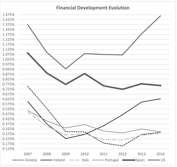
Data on financial development are obtained from the WDI version of April 2017, described in Beck et al. (2003). In line with the literature on financial development, we use an aggregated indicator which proxies for financial development. We use one indicator capturing the development of the stock market which provides the so-called “arm’s-length finance” (Levine, 2006). This indicator is a proxy for the size of the stock market. A larger market size indicates that investors are confident in the ability of the markets to channel funds into the most efficient projects (Tsoukas, 2011). The evolution of financial development indicators over time is provided in Figure 1.
<insert figure 1>
For comparison purposes, we illustrate FD ratios over the whole sample period for Greece, Ireland, Italy, Portugal and Spain, along with the ones for US. It is observed that during this time period, Euro area economies have a lower stock market indicator when compared to the most financially developed markets such as the American ones. We also observe a sharp decline during the global financial crisis in 2007-2009 for all countries. During the sovereign debt crisis period of 2010-2012 periphery countries’ ratios continue to further drop, with the exception
18 of Ireland. The figure illustrates that US stock markets are more liquid than Eurozone periphery ones, which may reflect the greater capital market development of the former. This is consistent with the idea that Eurozone economies, and especially those at the periphery of the Euro, have barely grown their capital markets during the period under study and that their financial structure has become strongly bank-based (loan-based finance). This could suggest that less market-oriented economies are more exposed to risk. Overall, these preliminary results show that banks’ efficiency levels may be related to the level of risk they face, the financial crisis and the level of capital market development. In light of the above, in the next section we summarize all the empirical results obtained from DEA-MPI and DBTR analyses and contextualize the relations between these variables.
4. Empirical results
4.1 First-stage results: DEA-MPI
The DEA-MPI results are presented in this section. As mentioned earlier, following Färe et al. (1994) the TFPCH is decomposed into its components EFFCH, TECHCH, PECH and SECH. This decomposition is valuable for our empirical setting, since it provides insight on the sources of overall productivity change in the domestic periphery banks. Practitioners can extract valuable information from evaluating the original MPI scores, rather than the bootstrapped ones, as bootstrapping is done usually to avoid serial correlation observed when the original scores are interacted with environmental variables. These estimates are summarized in Table 2. <Insert Table 2>
Overall, from the original DEA-MPI estimates several interesting findings are observed. Throughout the whole sample period, peripheral domestic banks exhibit improvement in their efficiency. This result is consistent with most of the components across countries. For example, Portuguese banks exert the highest productivity growth of 2.5% during 2007-2014, while Spain, Greece, Italy and Ireland follow with 2.2%, 2.1%, 1.9% and 1.2% respectively. From the decomposition of the MPI, this growth is driven mostly from the technological component (TECHCH) rather than the technical efficiency one. For example, Italian TFPCH is driven by +1.4% in technological efficiency and +0.2% in technical efficiency. Similar results are observed across all countries, except Spain where banks seem to ‘catch up’ to the frontier and turn towards the best practice in a similar fashion (+1.2% and +1.1% respectively). The decomposition into PECH and SECH shows different trends, but mostly that peripheral banks are improving their technical efficiency through the pure technical efficiency changes rather than
19 scale ones. For example, in Greece the 0.6% increase in EFFCH is driven by the 0.7% increase in PECH (as SECH is decreasing by 0.2%).
Examining the results in the pre-, post- and during the –Eurozone crisis, we see a clear pattern in the efficiency estimates. Namely, from 2007-2009 domestic banks’ efficiency is increasing overall. During the 2010-2012 crisis period the picture is vastly changing as high contractions in all efficiency metrics are observed. This is expected, as the Eurozone sovereign debt crisis vastly affected domestic banks’ operations. This can be explained by the fact that peripheral domestic banks became susceptible to a “moral suasion mechanism”. As described in Ongena et al. (2016), during this time peripheral governments prompted domestic banks to purchase additional amounts of domestic sovereign bonds and as a consequence became more exposed to their sovereign debt. In 2013-2014 a recovery in efficiency is observed. Between December 2011 and June 2014, banks had unlimited access to central bank liquidity, as long-term financing operations (LTRO) were done at a fixed rate. These LTROs targeted banks in GIIPS. According to Claeys (2014), the LTROs supported bank liquidity ensuring the finance of banks, subsidising the banking system and restoring its profitability. The estimated TFPCHs in Greece are indicative of the aforementioned clear pattern. In 2009 a +3.5% in productivity growth is observed, the same figure drops by 4.8% in 2011 and reverses in 2013 by a +3.1%. The worst results in terms of the different metrics of efficiency during the crisis are presented in the case of Italians and Spanish banks. This is expected as it is known that Italian and Spanish domestic banks actively purchased higher amounts of sovereign debt during the crisis than the rest of the periphery banks (Acharya and Steffen, 2015). The patterns observed in the whole sample regarding the different efficiency components remain similar when looking at the different periods and across countries. This is also illustrated by the following figure. <insert figure 2>
The above results provide a relatively uniform shape in the way domestic banks’ efficiency is evolving through time in the Eurozone periphery countries. Many researchers raise the question of whether European banking markets are integrated, homogenous and comparable. Usually, the presented results are mixed (see amongst others Weill (2004), Berger (2007), Bos and Schmiedel (2007) and Casu et al. (2016)). Our results are in a way in line with some of the results of Casu et al. (2004) and Casu et al. (2016). To the best of our knowledge, though, this is the first study that provides clear evidence of the existence of an efficiency meta-frontier specifically for European peripheral domestic banks. Given the above, it is now even more interesting to see how these results are affected by accounting for different bank- and country- specific variables. These are presented in the following section.
20 4.2 Second-stage results: DBTR empirical findings
4.2.1 Baseline models
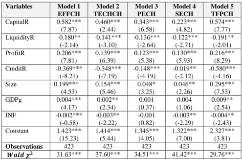
Table 3 reports the DBTR estimates for the baseline specifications (equation 10). The empirical findings are provided for all five estimated elements of DEA-MPI efficiency (EFFCH, TECHCH, PECH, SECH and TFPCH in column 2, 3, 4, 5 and 6 respectively). <insert Table 3>
Starting with capital risk (CapitalR), it positively affects the efficiency of domestic banks. More capitalised banks (financed with less leverage) are more efficient and face lower costs of going bankrupt over the 2006-2014 period. The relationship between capital risk and bank efficiency is not only statistically significant but also economically important. To illustrate the effect, let us consider the coefficient of CapitalR as shown in Column 2 of Table 3. The coefficient of 0.582 implies an elasticity of changes into best practice of the banks, evaluated at sample means of 0.044. A 10 percent increase of capital risk increases the banks technical efficiency by 0.44 percent. This is in line with previous studies (Sufian, 2014).
The results regarding liquidity risk are uniform across all estimated equations, demonstrating a negative and statistically significant relationship. It seems that there is a positive relationship between banks’ efficiency and the level of liquid assets held by the banks. Since higher figures of the ratio indicate lower liquidity, the empirical findings imply that domestic banks which are less liquid are also less productive. The economic significance of this variable is clear. The coefficient in Column 3 of -0.141 implies an elasticity of technology changes, evaluated at sample means of -0.063. A 10 percent increase of liquidity risk reduces TECHCH by 0.63 percent. The above discussion is in line with the argument that banks with higher loans in their assets portfolios increase the cost for their screening and monitoring, since loans are the assets leading to high operational costs (Naceur and Ghazouani, 2007).
The coefficients of ProfitR, the proxy for the degree of banks’ profitability, are positive and significant for all measures of bank efficiency. This suggests that higher levels of profits increase the ability of banks to be more efficient. This finding is also economically important. Looking, for example, at the coefficient of ProfitR in column 4, it indicates that a 10 percent increase of profitability raises the technology that shapes banks towards the best practice by 0.030 percent. This is in line with our expectations, since evidence presented by other studies such as Chortareas et al. (2013) and Sufian (2014) also reveal a positive effect of ROA on banks’ efficiency.
21 Credit risk (CreditR) exerts a negative effect and it has a highly statistically significant impact on banks’ level of efficiency for all models. Greater credit risk reduces the degree of bank efficiency. This illustrates the common knowledge that banks attempt to maximise their efficiency by adopting a risk-averse behaviour, which improves their screening process and tightens their risky loans’ monitoring. The magnitude of this effect is also economically relevant. Considering column 6, the coefficient on credit risk denotes an elasticity evaluated at sample means of -0.008. Hence, a 10 percent increase of credit risk contributes to a decline of the overall efficient of the banks of 0.08 percent. This is in line with other studies which find a negative effect for Brazilian banks (Staub, 2010) and Greek banks (Athanasoglou, 2008 and Delis and Papanikolau, 2009).
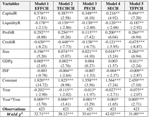
With respect to our bank-specific controls, Size (i.e. the log of total assets) exhibits a positive and a statistically significant relation with bank efficiency for all the models in Table 3. This finding is in line with previous theoretical and empirical evidence, which shows that banks with larger size reduce the cost of gathering and processing information (Staub et al., 2010). Finally, looking at the other control variables, it is clear that macroeconomic factors such as GDPg (INF) exert a positive (negative) and statistically significant effect on banks’ efficiency. The point estimates on inflation provide evidence that domestic banks are not able to target inflation correctly, which may lead to imperfect interest rate adjustment and potential losses (Pasiouras and Kosmidou, 2007). The positive effect of GDP growth is consistent with the well-known argument that economic growth is associated with positive performance of the financial sector (Pasiouras and Kosmidou, 2007). Finally, trend components are taken under consideration as a robustness check. The results obtained are consistent with the results of Table 3 and are presented in the Appendix.
4.2.2 Direct and indirect effects of the crisis on banking efficiency
To account for the role of the sovereign debt crisis on banks’ efficiency, we focus on its direct effect (equation 11). The aim is to evaluate the marginal impact of the crisis on the level of efficiency of domestic banks. Results are presented in the following Table 4. <insert Table 4>
The coefficients of the control variables retain their signs and significance after controlling for the direct effect of the crisis. The main risk variables also have the same significant effect. More importantly, the financial crisis attracts a negative and statistically significant effect for all different measures. Considering that the sovereign debt crisis led to a deterioration in the sovereigns’ creditworthiness and consequently decreased the value of the banks’
22 large domestic government bond holdings (Acharya et al., 2016), we consider this as an expected outcome. This outcome is also in line with the work of Acharya and Steffen (2015) and Ongena et al. (2016) on European domestic banks mentioned in section 4.1. Additionally, as with our baseline model, we account for trend components as a robustness check. Once again these results are in line with the results of Table 4 and are presented in the Appendix. Both robustness checks (baseline models/direct crisis effects) outlined in the Appendix prove that banks’ productivity follows a parabolic trend with a trough in 2010-2012. The next step involves including interactions between the four types of risk and the crisis term as in equation 11. This illustrates the indirect effect of the crisis to the operations of peripheral domestic banks. These results are presented in Table 5. <insert Table 5>
Comparing the role of capital risk during and outside of the crisis, we observe that bank efficiency is more sensitive to changes in the level of equity in the crisis. In other words, during the crisis banks are less capitalised (finance with more0.220 leverage) and as a result are less efficient. The smaller positive effect of capital risk on banks’ efficiency during the crisis means that banks face higher costs of going bankrupt, and therefore have a higher need for external funding which results in lower efficiency levels.
The vulnerability of banks to this position was highlighted with the onset of the Global financial crisis. In 2008, all banks in the Euro area were forced to enter into a deleveraging process and build more capital-intensive assets to reduce risk-weighted assets. However, banks at the periphery reshuffled their portfolio to sovereign bonds to relieve pressure on capital ratios and did not actually deleverage. This implication is consistent with the influential speech of Praet (2012), but also with the discussion paper of Lenarčič et al. (2016).
Banks’ efficiency levels are more sensitive to changes in the level of liquidity in the crisis period. The liquidity ratio exerts a higher (lower) impact during (outside) of the crisis. This is a novel result which suggests that there was an increase of risk during the sovereign debt crisis affecting banks’ liquidity risk and as a consequence their efficiency levels. The magnitude and the significance of the coefficients on the interactions with the crisis dummy are larger than the corresponding coefficients relative to the non-crisis period. These results confirm our hypothesis that the adverse effects of the sovereign debt crisis exert a stronger negative effect on the level of liquidity of banks. Banks’ large share of sovereign bond holdings increases their liquidity risk and therefore diminishes their efficiency levels. This implication is consistent with Acharya et al. (2016) who finds that banks in the GIIPS counties saw their levels of risk increasing as they held higher amounts of domestic government debt.
23 Turning to the remaining interaction terms, ROA still exerts a positive and statistically significant effect on two measures of banks efficiency. However, the effect is lower during the financial crisis than out of it. This is an expected result, as banks tend to be more productive, when they are able to attract higher levels of deposits and find creditworthy borrowers. During the sovereign debt crisis, periphery banks faced lower levels of profits and were induced to buy sovereign debt securities to improve their level of profitability (Ongena et al., 2016). Credit risk continues to have a negative effect on bank efficiency which appears stronger during the crisis than outside. This means that non-performing loans have a higher negative effect on bank efficiency during the crisis. In other words, periphery banks with higher credit risk tend to be less efficient during the crisis than outside the crisis period. This is expected as periphery banks are exposed to more high-risk loans during the crisis, which consequently can increase their vulnerability. This finding is in line with previous empirical evidence which shows that the changes in sovereign debt in countries such as Portugal and Greece positively affects banks credit risk (Acharya et al., 2016).
4.2.3 Financial development effects on banking efficiency
Having identified a direct and indirect effect of the financial crisis between risk ratios and banks’ efficiency levels, we also take into account whether this link varies according to the financial development level of the countries in which the banks are located. Table 6 shows the estimates for the interaction terms between the financial risk ratios and FD and (1-FD) dummies. The results reveal the heterogeneity between countries which is masked in the estimates for the full sample. We start with the discussion of the results presented for capital risk ratio. Our results seem to suggest that bank efficiency is more sensitive to changes in the capital risk ratio for lower levels of financially development and during the crisis. Banks in less (more) financial developed economies are less (more) efficient as they are more (less) likely to have higher (lower) leverage increasing their insolvency risk.
Next, we compare the coefficients of LiquidityR. Results indicate that the magnitude and significance of the interactions with the 1-FD term are larger than the corresponding coefficients related to the FD term. It shows that liquidity risk exerts a higher impact on banks’ efficiency for lower levels of financial development, especially during the crisis. This is an important result since it suggests that banks highly exposed to their countries sovereign debt have higher liquidity risk ratios and as a result, they have more difficulties in raising funds from new external sources which reflects their lower levels of efficiency. When profit risk (ProfitR) is considered, it is clear that banks