Selective randomized load balancing and mesh networks with changing demands

(1)

Selective randomized load balancing and mesh

networks with changing demands

F. B. Shepherd and P. J. Winzer

Abstract— We consider the problem of building cost-effective networks which are robust to dynamic changes in demand pat-terns. We compare several architectures based on using demand-oblivious routing strategies. Traditional approaches include single-hop architectures based on a (static or dynamic) circuit-switched core infrastructure, and multi-hop (packet-circuit-switched) architectures based on point-to-point circuits in the core. To address demand uncertainty, we seek minimum cost networks that can carry the class of hose demand matrices. Apart from shortest-path routing, Valiant’s randomized load balancing (RLB), and VPN tree routing, we propose a third, highly attractive approach: selective randomized load balancing (SRLB). This is a blend of dual-hop hub routing and randomized load balancing which combines the advantages of both architectures in terms of network cost, delay, and delay jitter. In particular, we give empirical analyses for the cost (in terms of transport and switching equipment) for the discussed architectures, based on three representative carrier networks. On these three networks, SRLBmaintains the resilience properties ofRLB while achieving significant cost reduction over all other architectures, including RLB and multi-hop IP/MPLS networks using VPN tree routing.

I. INTRODUCTION

Emerging data communication services create an increasing degree of uncertainty and dynamism in the traffic distribution across carrier networks. Examples are virtual private networks (VPNs) as well as remote storage and computing applications [3], [1]. For network design purposes, such services are best captured by the hose model [7], [10], which treats the node ingress/egress capacities as known constants, but does not specify point-to-point demands. For example, the service level agreement (SLA) for a VPN customer who wants to interconnect several business sites using a carrier’s network could just specify the peak rates at each ingress node, but leave open the distribution of traffic to be sent between each node-node pair. It is then up to the carrier to efficiently route the traffic over the network.

Contemporary carrier networks are often built on circuit-switched core technologies (‘IP-over-SONET’), which offer high reliability and fast protection schemes. However, when traffic demands change over time, traditional circuit-switched network architectures lack bandwidth efficiency, which can lead to a severe underutilization of network resources. Moder-ate degrees of traffic dynamics, such as diurnal demand varia-tions, can potentially be handled by advanced control plane concepts (e.g., the automatically switched optical network ASON based on generalized multi-protocol label switching, GMPLS [29]), but rapidly changing demand patterns cannot. In contrast, packet-switched backbone architectures

(‘IP-over-WDM’) provide the benefit of statistical multiplexing, and thus allow for a better utilization of network resources without the need for a dynamic control plane. However, there are significant drawbacks arising from purely packet-switched architectures. First, packet-switched networks examine and route the traffic at each node along a source-destination path. As we will see below, this comes at a considerable cost, since packet router ports are substantially more expensive than the equivalent ports on a circuit-switched crossconnect [24]. This fact continues to hold for MPLS networks based on IP/MPLS routers, since MPLS label lookup is inherently more involved than SONET crossconnecting. In addition, for larger networks, the need for routers to establish connectivity in the core can become a node scalability problem due to the difficulties in scaling packet routers [15]. Second, packet-based networks, by their very nature, use buffering at each node, which introduces packet loss and delay jitter, and makes quality-of-service (QoS) guarantees difficult to achieve. Third, packet-switched core networks do not meet the reliability and restoration constraints granted by circuit-switched networking infrastructure.

In an effort to combine the advantages of circuit-switched and packet-switched network architectures for rapidly chang-ing demand patterns, references [16], [20], [27], [21], [28] apply Valiant’s scheme of randomized load balancing (RLB) [25] over a circuit-switched network. This previous work has focused on a variety of network performance measures including throughput, link congestion and switch fanout. The basic idea of RLB (see Section IV-B) is to route demands from network edge nodes in two phases. In the first (load balancing) phase, all nodes randomly distribute their traffic among all other nodes. In the second (routing) phase, each node processes the packets it received in phase 1, and sends them to their final destination. Since each packet is only processed once on its path from source to destination, the need for multi-hop packet routing using core routers is greatly reduced. In each of the two phases, traffic is carried on cost-effective circuit-switched (layer 1) core technology, without having to experience layer 2 or 3 processing at each node. The resulting RLB network offers SONET-grade reliability, and in many cases promises lower deployment cost than conventional architectures designed for dynamic traffic variations. Further-more, delay jitter and QoS guarantees are likely to be met more easily than in packet-switched architectures, since all packets experience only a single stage of routing (and therefore only a single stage of buffering).

(2)

Hub

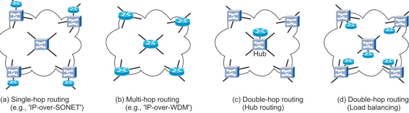
(a) Single-hop routing (e.g., 'IP-over-SONET') (b) Multi-hop routing (e.g., 'IP-over-WDM') (c) Double-hop routing (Hub routing) (d) Double-hop routing (Load balancing)

Fig. 1. Network architectures considered in this work. (Square network elements: Circuit-switched crossconnects. Round network elements: Packet routers.)

Our Results

In this paper, we first address some inherent drawbacks associated with RLB. Most notably, we explore the ineffi-ciency in distributing all traffic across the entire network. Based on these observations, we propose selective randomized load balancing (SRLB) [27], where RLB is performed across a limited number of carefully chosen hubs in the network. We point out the advantages of SRLB over the other architectures discussed in this paper. After computing an optimal set of hubs, we are able to give empirical evidence that SRLB is an attractive architecture combining the distinct advantages of RLB (resilience) and VPN tree routing (network cost).

This paper is organized as follows. In Section II we give an overview of the considered network architectures, including some important definitions. In Section III we give some back-ground on models for uncertain demands, robust optimization, and oblivious routing. In Section IV we discuss two important examples of oblivious flow templates: shortest-path routing and VPN-tree routing. We show how previous work on VPNs can be applied to avoid excessive processing costs at the nodes. We observe that RLB can use significantly more link bandwidth than an optimal VPN tree network, which moti-vates the introduction of SRLB in Section IV-C, forming the conceptual core of this paper. Section V is the main empirical section and provides detailed results based on the cost of the network elements needed to build the different architectures studied. We show by means of empirical examples how SRLB lowers network cost and improves delay jitter. In Section VI we then discuss resource utilization for different network architectures and flow templates, and show to what extent (depending on the flow templates) resource under-utilization can become an advantage for IP/MPLS networks through statistical multiplexing in the presence of best-effort traffic. In this context, we also introduce the notion of the robustness premium to quantify the amount of over-provisioning that is needed to accommodate dynamic traffic demands. Finally, we conclude in Section VII.

II. NETWORKARCHITECTURES

Circuits

A circuit is defined by two endnodes and some provisioned, dedicated capacity in a physical network. This capacity can be viewed as a point-to-point pipe that carries traffic unaffected between the specified endnodes of the circuit, with no packet processing, header lookup, or label lookup required along the way. In practice, a circuit may be implemented within the SONET hierarchy, or it may be a full wavelength channel in an optical network using optical add/drop multiplexers (OADMs). Note that an MPLS-‘circuit’ is not a circuit within this definition, since MPLS requires packet processing in the form of label lookup at each node from source to destination. The role of MPLS will be discussed in detail in Subsection VI-D.

Packet (hop) routing and circuit provisioning

All network traffic reaches its destination by following a sequence of circuits or hops; the particular choice of a sequence of hops is referred to as the hop routing. If traffic follows several hops, the intervening nodes, called routing nodes, must support the functionality to route traffic onto the next hop towards its destination. This may for instance be achieved by examining each Ethernet frame, IP packet header, or MPLS label in between two hops using Ethernet switches or IP/MPLS routers (interconnected by SONET or wavelength-division multiplexed (WDM) circuits).

Circuit provisioning constraints specify how individual hops are implemented in the physical network. Most standard is that a circuit is identified with a single, capacitated path between its endpoints, but one may also consider circuits implemented as fractional flows; this is also called multi-path routing, and is implemented, e.g., using virtual concatenation and the link capacity adjustment scheme (VCAT/LCAS). In addition, the circuits used by hop paths may be provisioned statically or dynamically; in the latter case, the physical layer needs a control plane that dynamically adapts to changing traffic patterns (e.g., ASON/GMPLS).

Network architectures

A network architecture refers to a collection of constraints on how data is routed at the packet layer. The architectures

(3)

we consider are: single-hop routing, hub routing (dual-hop routing via one node), Valiant’s randomized load balancing and selective randomized load balancing (dual-hop routing via all [RLB] or a selection of [SRLB] terminal nodes), and multi-hop routing (no bound on the multi-hop length).

Given an architecture, there exist several physical imple-mentations of the network depending, for instance, on the choice of switching (node) equipment.

Examples

We now discuss several concrete examples of the abstract architectures considered. Figure 1(a) depicts a single-hop network architecture, where packets are routed at the ingress, where they are placed onto pre-defined circuits, and traverse a circuit-switched core network to their destinations. If static circuit provisioning is employed, each node-node pair (i, j) has to be connected by a circuit of capacity equal to the maximum possible demand between i, j. Since every circuit can handle the entire demand originating at a node without re-configuration, no control plane is needed, but the architecture results in a vast over-provisioning of network resources if traffic patterns are allowed to vary significantly. This can be mitigated by using dynamic provisioning of circuits by means of a dynamic control plane, setting up and tearing down circuits as needed, and thus allowing traffic to share core network resources. This approach is severely limited however by the speed and complexity of available control plane technologies.

Figure 1(b) depicts a multi-hop architecture. Here, each core node examines the traffic entering it on a circuit, and places it on a different circuit following a locally implemented routing strategy. The best-known example for this architecture is an IP/MPLS network, where nodes are IP/MPLS routers and circuits are point-to-point line systems (e.g., WDM links) between them. From a capacity analysis viewpoint, the multi-hop architecture is equivalent to a single-multi-hop architecture with a sufficiently fast control plane to support traffic dynamism. The role of the globally acting control plane is taken over by statistical multiplexing through local packet routing.

Figures 1(c) and (d) depict the two extreme cases of double-hop architectures. Here, traffic is first sent to one (c) or more (d) intermediate routing nodes using preset circuits, irrespec-tive of the traffic’s final destination. The intermediate nodes perform local routing decisions, and again use the circuit-switched core to deliver traffic to its final destination. The case of a single intermediate routing node [Figure 1(c)] is called a hub routing architecture. Although using a single hub often leads to lowest overall network cost, it is not the most desirable architecture in practice, since the hub (i) represents a single point of failure, and (ii) has to route the entire network traffic, which can quickly become a network scalability problem. The case where incoming traffic is distributed across all nodes [Figure 1(d)] is inspired by Valiant’s randomized load balancing, introduced in the context of parallel computing [25] and discussed further in Section IV-B.

III. TERMINOLOGY ANDBACKGROUND

We consider network design where we are given a physical network represented by a graph G = (V, E). The set V represents node locations, and E is the edge set, represent-ing which nodes pairs are joined by a physical link. Our assumption is that each edge has an abundance of channels (for instance, fibers) and that network cost is mainly associated with (i) activating these channels (for instance, installing line terminal equipment or optical amplifiers along the line) and (ii) populating the nodes with the appropriate switching equipment (packet routers, SONET crossconnetcs, etc.). Thus for our purposes, we view each edge e ∈ E as having an unbounded supply of bidirectional (undirected) links, each with an associated cost for activating. The full cost model will be discussed at length in Section V.

We also have a specified set of edge nodes (sometimes called terminals), where traffic is injected into the network. Normally, we take the set of edge nodes to be the whole setV (but the algorithms work for any proper subset). Even though our edges are undirected, we maintain the convention that demands may be oriented; that is, there may be distinct unidirectional demands from nodeito nodej, and from node j to nodei. In our numerical implementations, we normally think of these demands as being paired, and then routed on bidirectional path(s). Traffic is then specified by a demand matrixdij. We refer to the valuePjdij (resp.Pjdji) as the

ingress (resp. egress) traffic at i. We assume throughout that there is a bound denoted byDi (also called the marginal) on

both the ingress and egress traffic at i. Uncertain Demands and Robustness

Network designers have traditionally adopted the view that an accurate estimate for point-to-point traffic is given prior to laying out circuits. The increasing importance of flexible data services has led to situations where traffic patterns are either not well known a priori or are changing rapidly. In these settings the network should be dimensioned to support not just one traffic matrix, but a large class of matrices determined by the application.

This scenario leads to a robust optimization problem: given a universe U of so-called valid demand matrices (normally specified as a convex region), the goal is to design the network so that every demand matrix in U can be supported at the lowest possible cost. The simplest form of this problem, recently shown to be NP-hard [6], is to allocate fractional link capacities that are sufficient to support a multicommodity fractional routing for each demand matrix in the universe U, where the fractional routing used may change dynamically if the demand matrix does.

Motivated by the application of supporting uncertain or changing demands, the focus of our study is on the universe of hose matrices. In the hose model, there is a subset of nodes that inject traffic into the network. For each of these nodesi, we have a bound Di which is an upper bound on the total

demand that this node may offer (ingress capacity) or receive (egress capacity). Note that in general, these bounds could

(4)

be independent of each other The class of hose matrices for the marginal values Di is then U = {dij ≥ 0 : Pjdij ≤

Di,Pjdji≤Di, ∀i}. Recall, that we do not in general have

to assume symmetric demands, nor do we have to assume anything about demand from i to j using the same path as that from j toi (though in fact we could if we wish without changing the results).

It is obvious that in general one must pay more to be able to support a whole class of demand patterns rather than just a single traffic matrix. We refer to this factor increase in cost as the robustness premium, and will report on its value from our experiments in Section VI-E.

Oblivious routing and flow templates

The capacity required to support a class of traffic ma-trices obviously depends on the degree to which network elements can use current information about the network topol-ogy and utilization of network resources, for determining a cost-effective routing of the existing demands. Real-time re-provisioning of circuits in physical core networks to adapt to changing demands is not generally available. In contrast, packet switches (IP routers or Ethernet switches) have some ability to adapt traffic routes in real-time, but this leads to a network management overhead since complex traffic engineering may be needed. For these reasons, in our study, we restrict ourselves to oblivious (sometimes called static [4]) routing strategies, which depend only on the network topology, but are agnostic of network utilization parameters or current traffic distributions.

Formally, an oblivious routing is determined by a flow template. A flow template for a specific node pair (i, j) specifies how to send one unit of flow from i to j. Hence it can be modeled as an assignment f(P)to each i−j path so that P

P∈Pijf(P) = 1. (We use Pij to denote the set of paths (usually simple) between i and j.) If our network is currently handling a traffic matrix d, then the interpretation is that it treats the i to j traffic as follows: for each i−j -path P, it sendsf(P)dij flow along path P. Naturally, flow

templates can be fractional (multi-path routing) or single-path (unsplittable flow), or may obey some other restrictions, for instance bounds on path length. A flow template, usually denoted by f, then consists of a template for each pair of nodes i, j that are injecting traffic into the network. We have defined our templates in terms of a path variable; compact arc/edge formulations could have also been used as is done in [2], [9] for related problems. To avoid confusion, we note at this point that an oblivious routing strategy does not actually define a hop routing since it does not specify at which nodes packet routing is actually performed. Rather, flow templates specify the flow of traffic at the physical layer.

Optimization of demand-oblivious routings (for any network performance measure including cost) can be challenging since flow templates seek to perform resource sharing between different demand matrices. Work on finding efficient demand-oblivious routings for robust networks has focused on choosing the universeU to be the matrices arising from the hose model

[7], [8], [9], [10], [11], [12], [14], [22]. We will be especially interested in work of [11] on the uncapacitated, undirected version of the hose model with equal bounds on ingress and egress capacities. A different setting is considered in [23] where an efficient oblivious routing (with respect to link congestion as opposed to network cost) is described for the universe of demand matrices that are routable in the existing network (cf. also [6]).

We mention that the worst-case concept of robustness is only one way to approach uncertainty in optimization data. Others include chance-constrained optimization and stochastic programming. We refer the reader to [18] for an application of the latter approach to network design and subsequent augmentation.

IV. EXAMPLES OFFLOWTEMPLATES ANDSELECTIVE RANDOMIZEDLOADBALANCING

We consider several flow templates for oblivious routing: shortest path routing, tree routing, hub routing and randomized load balancing. We see that in uncapacitated networks, RLB can be viewed as a ‘convex combination’ of hub routing templates. This leads us to propose an intermediary selective randomized load balancing scheme.

A. VPN Trees and Hub routing

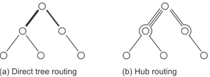
In this subsection, we will discuss tree networks as highly attractive topologies to support hose traffic. As will become obvious in Section IV-C, these discussions are crucial to transition from RLB to the newly proposed SRLB architecture. Given any fixed tree T that contains all edge nodes, the capacities required to support all traffic under the (undi-rected/bidirectional) hose model are readily computed as fol-lows. For each edgee∈T, consider the two sub-trees obtained after deleting e. Let B be the smaller of the total marginal capacities (i.e., the sum of the node ingress/egress capacities) in each of the two sub-trees. One easily sees that there is a valid hose matrix that simultaneously sends B demand from the smaller sub-tree to the larger sub-tree and vice versa. Thus, if all hose matrices ought to be routed on T, emust support a bidirectional capacity of at least B. We refer to the link-capacitated tree resulting from repeating this calculation for each edgee as the VPN Tree associated with T, and denote it by VPN(T); the name is inspired from the application to virtual private networks considered in [11]. The link capacities on any VPN Tree are sufficient to route every hose traffic demand if we use the following oblivious flow template: demand between any node pair i, j routes along the unique shortest path between i and j in T. We call this oblivious flow template the tree template associated withT. An elegant method for computing the optimal VPN Tree is derived in [11].

We also consider a second flow template on trees, called the hub routing template. For any treeT and nodev consider the flow template where every incoming demand first sends traffic to the hub nodev, and thenv forwards the demand to its final destination. Using this template, the link capacities

(5)

(a) Direct tree routing (b) Hub routing

Fig. 2. Tree routing (a) and hub routing (b) make use of different circuits (represented by lines), yet sometimes require identical edge capacities.

required to support every hose matrix are easily computed. Namely, consider the load on each edge when the edge nodes isimultaneously sendDibidirectional traffic to the hub node

v. We denote the resulting link-capacitated tree asHUB(T, v). It is easy to check that any edge in HUB(T, v)is assigned at least as much capacity as it is in VPN(T).

In their study of the VPN problem, [11] show a connection between the two types of capacitated treesVPN(T),HUB(T, v). Namely, they show that there is an optimal capacitated tree (in terms of link capacity), denoted here by Topt, with the

following simple structure. There is a nodersuch that this tree is a shortest path tree1_T

rrooted atr. One consequence is that

one may arrive at an optimal VPN tree by simply solving for a shortest path treeTvfrom each nodevand taking the cheapest

of all resulting trees. A more important consequence is that in the optimal tree, their proof shows that VPN(Tr) is precisely

the same as HUB(Tr, r). Thus there is enough capacity on the

tree to use either the tree flow template as is done in [11] or the hub routing flow template. This is significant for us since we can implement a hub routing template via highly cost-efficient statically provisioned circuits between each node and the hub. In contrast to [11] where the focus is on link costs, this becomes significant for us since it eliminates the need to perform packet routing operations at nodes between source and destination, as would be required for tree routing. The difference between the two strategies is visualized in Figure 2. In the remainder of the paper we use VPN-tree and VPN-hub to denote using the tree and hub flow templates respectively, on an optimally designed tree VPN(Topt), defined above.

We close by mentioning that in [11] it is shown that the cost of VPN(Topt)is within a factor 2of the optimal possible

by any fractionally capacitated network. It remains an open problem to determine whether it is in fact optimal! (cf. [13]). B. Randomized load balancing (RLB)

Randomized load balancing is a two-step (double-hop) rout-ing scheme based on a statically provisioned circuit-switched core. In a first (load balancing) phase, traffic originating at any node of an N-node network is uniformly distributed among all N nodes. For example, in the case of equal node ingress/egress capacities, each node distributes 1/N-th of its 1_{If only some of the nodes are terminals, the tree is obtained by routing}

each edge node toralong a shortest path to obtain a ‘cheapest flow tree’ that contains all edge nodes.

traffic to each other node (and keeps 1/N-th to itself). The traffic distribution in Phase 1 is random in the sense that it is totally agnostic of the demand matrix and does not require any routing decisions at the ingress. In Phase 2, each node performs local routing decisions on the traffic received in Phase 1, and statistically multiplexes the traffic onto circuits leading to its final destination. Due to the random and uniform distribution of traffic in Phase 1, the traffic distribution in Phase 2 will also be uniform on average, with fluctuations being accommodated by buffering within the routing nodes.

We now discuss some of the concrete advantages, issues, and solutions associated with implementing RLB in practice. Hardware Benefits: The link capacities required to perform the two phases of RLB are readily obtained as follows [10], [11], [16]. For traffic marginalsDiat the nodes, the amount of

traffic distributed in each phase is the product multicommodity flow [17] induced by theDi’s, i.e., the traffic between nodesi

andj isDiDj/PlDl. Note that the uniform nature of traffic

in Phases 1 and 2, regardless of the actual demand matrix to be routed, permits pre-allocation of static network circuits, which dramatically simplifies network design.

Since each node j receives a total of P

iDiDj/PlDl =

Dj from all N nodes (including itself), the node routing

capacity required for Phase 2 equals the total node ingress capacity. This corresponds to the routing capacity required for source-routed (single-hop) network architectures. However, full support of dynamically changing demand patterns is maintained through local routing, and no global control plane is needed.

Resequencing, Delay and Jitter: Since RLB performs strict double-hop routing, all traffic is buffered only once (at the beginning of Phase 2). This reduces random buffering delays when compared to a multi-hop network architecture, which buffers traffic at each node. One obvious disadvantage of RLB (as with any other architecture employing multi-path flow templates) is the routing of traffic over paths with significant time-of-flight differences. The resulting delay spread poten-tially asks for packet re-ordering. Note, however, that these time-of-flight differences do not contribute to random delay jitter, but are fully predictable based on knowledge of the hop routing and flow template, and can thus be counteracted by deterministic delays at the ingress, intermediate, or egress nodes. Alternatively, traffic splitting at the ingress node can be performed on a per-flow basis, as explained below. The maximum propagation delay in RLB is about twice the time-of-flight of the longest path in the flow template, which restricts the geographic dimensions of such networks. Resilience and Security: Due to the distribution of traffic among all routing nodes in Phase 1 of RLB, the architecture is inherently vulnerable to routing node failures. However, RLB uses a multitude of routing nodes, as opposed to the hub architecture, in which the routing hub represents a single point of failure. Therefore, RLB can be made robust to routing node failure either by means of error-correcting coding or by means of back-pressure protocols that throttle the ingress traffic by

(6)

Randomized load balancing =

+

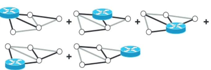
Fig. 3. RLB is a convex combination of hub routing templates. For each root nodev, edges that are part ofTvare shown in black.

1/N should a routing node fail. Another interesting aspect of distributing the traffic across the network is the resulting resilience to eavesdropping attacks. In order to successfully intercept information, an adversary has to tap into almost all routing nodes. In conventional network architectures, tapping into a single routing node or into a single link can be sufficient to fully intercept information.

In closing, we want to mention that RLB can either be performed on layer 2 (Ethernet) or layer 3 (IP). Within each implementation of RLB, there are several traffic splitting strategies. For example, by properly controlling the traffic splitting at the ingress node, one can either make sure that flows are kept together and are thus always routed along the same paths, or that flows are always split up on a per-destination basis. While the first option entirely eliminates the resequencing problem, it may reduce the traffic uniformity established in the load balancing phase in the presence of exceedingly large flows. The second option insures uniformity but it requires a smart ingress capability which adds an expense to edge router equipment.

C. Selective Randomized Load Balancing (SRLB)

From a network capacity point of view, the optimum VPN tree networkVPN(Topt)(using either the tree flow template or

the hub routing template) is always as good as (and usually better than) using RLB. To see this, notice that Phase 1 traffic (as well as Phase 2 traffic) in RLB can be written as a 1/N convex combination of N capacitated trees arising from routing Di flow from each i to the root of a shortest path

tree Tv, for each nodev∈V (or each edge node in general).

Thus, the total capacity required by RLB is a 1/N convex combination of the capacitated trees HUB(Tv, v). The cost of

RLB is then at least the cost of VPN(Topt)by the following

argument. We have seen in Section IV-A, that the total capacity cost ofHUB(T, v)(for anyT, vand hence also forTv, v) is at

least as large as that of VPN(T). Moreover, the total capacity cost of VPN(T) for any treeT (and in particular for anyTv)

is at least as large as the capacity cost of an optimal VPN tree Topt. Thus the RLB capacity is a convex combination of

trees, each of whose capacity cost is at least as large as that of Topt. Figure 3 visualizes this important observation.

As a consequence, we introduce SRLB as a blend of the two dual-hop architectures by performing RLB over those M < N hubs that are associated with theM best shortest path trees (computed over all nodes as hubs). The cost criterion for

computing theseM best trees may be based on, e.g., network cost or on minimizing differential delay. For example, if the objective lies in minimizing network cost, one first calculates the cost of all N shortest path trees (one for each node), and simply picks theM lowest-cost trees. One then performs SRLB using the hubs from the selected trees.

With respect to reducing propagation delay and delay spread, we note that the hubs associated with theM lowest-cost trees are typically clustered together near the center of the network; the “center” is characterized by the notion that the aggregate traffic on all edges connected to the center is best possibly balanced, reflecting directly the construction of the VPN tree [11]. Since lowest-cost nodes tend to be clustered together, the difference between the transport distances for any demand using these nodes as a routing hub is minimized. This mitigates one severe drawback of randomized load balancing: the different delays of packets distributed to different interme-diate nodes (delay spread) and the potential resulting need for packet re-sequencing.

Another drawback revealed in our empirical studies in Section V is that when switching equipment costs are included, network cost based on RLB may actually exceed that of multi-hop IP designs. In contrast, SRLB across a limited number of hubs yields designs cheaper than either RLB or multi-hop architectures. A quantitative comparison of SRLB to RLB and to conventional network architectures in terms of cost, delay, and delay jitter will be given in Section V.

V. COST COMPARISON AND RESOURCE REQUIREMENTS

In this section, we compare the capacity requirements for the architectures and flow templates introduced in Sections II and III, using the three example networks studied in this work, and depicted in Figure 4: the UK research network JANET, the US research backbone ABILENE, and the European research network GEANT.

We assume symmetric demands (dij =dji) and equal nodal

ingress/egress traffic (P

idij = D/N for each j). Demand

patterns are allowed to vary under the hose constraint, and all architectures are capacitated to accommodate all valid demand matrices.

As described in Appendix B, we use linear program-ming (LP) formulations to calculate the capacity requirements needed to support all hose demand matrices. Given a fixed flow template, one computes for each link/node the worst case capacity requirement needed to support every hose matrix. Each of these subproblems (one for each link/node) amounts to a so-called fractionalb-matching problems [9], [2].

The results are displayed in Tables I – III. The first columns specify the network architectures, and the second columns in-dicate the flow template used. The tables list the total required circuit-switching capacity (e.g., by SONET crossconnects), the total packet-switching capacity (e.g., by IP/MPLS routers), and the transport capacities (e.g., by WDM line systems) for different network architectures and shortest-path (SP) as well as VPN-tree templates. The right-most columns give the overall network cost, normalized to the hub architecture using

(7)

Glasgow Edinburgh Leeds Warrington Reading Bristol Portsmouth London

(a) JANET topology (b) ABILENE topology (c) GEANT topology

Fig. 4. Three example networks considered in this paper [http://www.ja.net; http://www.abilene.iu.edu; http://www.geant.net].

an optimum VPN Tree. In order to arrive at the overall network cost, we assume the following cost model for commercially available networking hardware [24], [21],

cIP-port:cSONET-port:cWDM/km= 370 : 130 : 1, (1)

wherecIP-portis the cost of an IP/MPLS router port,cSONET-port

is the cost of a SONET crossconnect port, andcWDM/kmis the

cost of WDM transport per km of link distance, all for the same data rate2. Since we are giving all capacity numbers as well as cost numbers, it is possible for the interested reader to plug any other suitable cost ratio into our results.

For the RLB architecture, we assume that those line cards on the SONET crossconnects handling the nodal ingress/egress traffic are equipped with means of packet (or flow) split-ting and, if required, re-sequencing. We allocate an addi-tional cost of half the cost of a standard circuit-switched line card to this functionality; thus, the per-port cost of an ingress/egress line card in the load-balanced architecture amounts to1.5cSONET-port.

For the circuit-switched network with dynamic control plane, we do not allocate any additional cost, since highly dynamic control planes do not yet exist, and a meaningful quantification of their cost cannot be given.

As is evident from the overview tables, the static single-hop architecture with its need for high over-provisioning leads to overly expensive network cost. Neglecting the dynamic control plane architecture for its lack of availability, the most important contenders for dynamic networking are the multi-hop architecture (3.), the RLB architecture (4.), and the hub architecture (5.). Of these three architectures, the hub architecture (using the optimum network node as a routing hub) proves cheapest on all networks, in agreement with the VPN-tree strategy [11], [22]. However, all traffic is processed in a single routing node that has to be able to handle the entire network traffic D. Therefore, this architecture incorporates a single point of failure, and is thus often considered unreliable. 2_{Note that our cost model breaks down cost directly to ports on routers or}

crossconnects. In practice, this is a justifiable simplification, since the cost of line cards typically dominates the cost of main frames.

Depending on the network size, we identify RLB across all network nodes to be lowest-cost on networks of smaller geographic size (JANET), while multi-hop VPN-tree routing performs better on larger networks (ABILENE and GEANT). This is expected from our previous discussions, since RLB in general uses up more transport capacity than VPN tree-based architectures, and can therefore only prove in if the cost of routing dominates the cost of transport. In fact, if we scale the ABILENE topology from its average link distance of 1,317 km down to 831 km, and the GEANT topology from an average link distance of 797 km down to 319 km, randomized load balancing exhibits equal cost to multi-hop routing on a VPN tree. For comparison, JANET has an average link distance of184 km, and randomized load balancing out-performs multi-hop IP routing up to an average link distance of 1,030 km on this topology. Note that conventional multi-hop routing on shortest paths is always more expensive than RLB on the studied networks.

Selective randomized load balancing

We now examine selective randomized load balancing (SRLB) across an optimally chosen subset of M hubs. The process for choosing the hubs is as follows (see also

Sec-Intermediate routing nodes (M)

Cost ratio (referenced to hub) 5 10 15 20 25 1 1 1.1 1.2 1.3 1.4 JANET ABILENE GEANT JANET GEANT ABILENE

Fig. 5. Cost of selctive randomized load balancing compared to cost of optimum hub routing as a function of number of intermediate nodes.

(8)

TABLE I JANET – OVERVIEW

Architecture Flow Circuit-switching Packet-switching Transport Cost ratio

Template capacity capacity capacity×km (to hub)

1. Single-hop SP 120 16 11,104 3.12 2. Single-hop SP 42 16 3,437 1.42 (dynamic) VPN-tree 32 16 2,302 1.18 3. Multi-hop SP – 42 3,437 1.81 VPN-tree – 32 2,302 1.35 4. Load-balanced SP 44 8 2,776 1.14

5. Hub routing VPN-hub 40 8 2,302 1.00

TABLE II ABILENE – OVERVIEW

1. Single-hop SP 287 22 165,478 6.07 2. Single-hop SP 71 22 37,019 1.57 (dynamic) VPN-tree 51 22 22,621 1.08 3. Multi-hop SP – 71 37,019 1.82 VPN-tree – 51 22,621 1.19 4. Load-balanced SP 72 11 30,087 1.27

TABLE III GEANT – OVERVIEW

1. Single-hop SP 2,157 54 760,210 15.87 2. Single-hop SP 223 54 69,142 1.77 (dynamic) VPN-tree 127 54 36,823 1.10 3. Multi-hop SP – 223 69,142 2.27 VPN-tree – 127 36,823 1.25 4. Load-balanced SP 212 27 56,312 1.43

tion IV-B): We evaluate the cost of each of the N possible single-hub architectures using shortest-path trees; the cheapest of these N hub architectures, routing on an optimal VPN tree [11], [22], is listed under (5.) in Tables I – III. The most expensive hub architecture exceeds the cost of the cheapest hub by 22%, 57%, and 90% for JANET, ABILENE, and GEANT, respectively. We then sort our N possible hub architectures in ascending cost, and pick the M lowest-cost hubs to perform SRLB.

Figure 5 quantifies the benefit of SRLB by showing the cost of a SRLB network, normalized to hub routing, as a function of the M lowest-cost intermediate nodes, taking into account the cost of the traffic-splitting and re-sequencing hardware. Comparing the curves with the cost numbers for multi-hop VPN-tree routing from Tables I – III, indicated by horizonal arrows to the right of Fig. 5, we see that SRLB on the ABILENE network performs better than multi-hop VPN-tree routing if M ≤ 8 intermediate nodes are chosen. On the GEANT network, M ≤ 13 intermediate nodes need to be chosen in order to compete against multi-hop VPN-tree routing. On the JANET network, RLB performs better than VPN-tree routing to start with, and SRLB is able to further reduce network cost.

As explained in Subsection IV-C, SRLB mitigates the delay

spread associated with the RLB architecture, since the lowest-cost hubs are located around the center of the network. To quantify this statement, we calculated the delay spread for RLB and SRLB on our three example networks. To this end, we evaluated, for every source-destination node pair i, j, the time-of-flight differences incurred by routing via all possible intermediate routing hubs. Our analyses show that the worst-case delay spread on the JANET network is cut in half by SRLB with 5 intermediate nodes instead of load balancing across the entire network. On the ABILENE network, the same reduction is obtained when using 6 routing nodes, and on the GEANT network when using 16 nodes.

VI. RESOURCE UTILIZATION,CLASSES OF SERVICE AND ROBUST DESIGN

In order to arrive at more detailed results for network capacity requirements, classes of service, and to study network resource utilization we followed two independent avenues. First, we performed extensive Monte Carlo simulations using ensembles of randomly chosen demand matrices satisfying the hose constraint. Second, we solved the inherent LP formula-tions for the problems. This allows for fast prediction of upper capacity bounds for each link and node. We combined the two approaches to measure resource utilization and the advantages

(9)

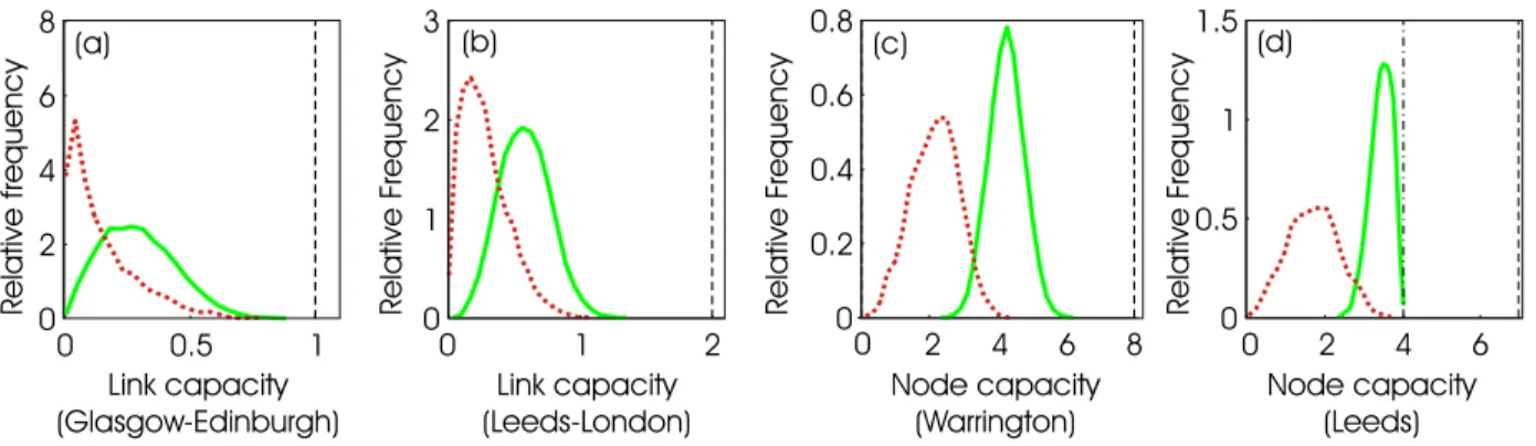
0 0.5 1 0 2 4 6 8 0 1 2 0 1 2 3 0 2 4 6 8 0 0.2 0.4 0.6 0.8 0 2 4 6 0 0.5 1 1.5 Node capacity (Leeds) R e la tiv e F re q u e n c y R e la tiv e F re q u e n c y R e la tiv e f re q u e n c y R e la tiv e F re q u e n c y Node capacity (Warrington) Link capacity (Glasgow-Edinburgh) Link capacity (Leeds-London) (a) (b) (c) (d)

Fig. 6. . Statistical analysis of the JANET network (100,000 realizations of a hose-constrained, random demand matrix). (a) and (b): Histograms of the traffic on the links Glasgow-Edinburgh and Leeds-London. (c) and (d): Histograms of the total traffic (add/drop and thru) handled by nodes Warrington and Leeds. Solid curves: Tight hose model (P

idij=D). Dotted curves: Weak hose model (0≤

P

idij≤D) with uniformly distributed node traffic. Dashed lines: Worst-case link capacities in (a) and (b); worst-case node I/O capacities in (c) and (d). Dash-dotted line in (d): Worst-case node switching capacity.

of IP/MPLS due to statistical multiplexing. A. Statistics through Monte Carlo simulations

We performed Monte Carlo simulations using ensembles of 100,000 randomly chosen symmetric demand matrices satisfying the hose constraint, i.e., dij = dji, dii = 0, and

P

idij = Pjdij =D ∀ i, j. All dij were allowed to vary

between 0 and D as long as the above constraints were met. The method of generating the random matrices is described in Appendix A. We routed each matrix individually across the network, using a fixed flow template (shortest-path3 For each matrix, we recorded the capacity needed on each link as well as at each node, leading to ensembles of 100,000 random link and node capacities, on which we performed statistical analyses. Figure 6 shows some selected results for the JANET network [Figure 4(a)] using shortest-path routing; (a) and (b) show histograms of the traffic flowing over two selected links (Glasgow-Edinburgh and Leeds-London), while (c) and (d) show histograms of the total traffic (add/drop plus thru) to be handled by two selected nodes (Warrington and Leeds). The solid curves correspond to the tight hose model (P

idij = D), while the dotted curves apply to the

weak hose model (0 ≤ P

idij ≤ D), where the total node

demands were allowed to vary randomly between 0 and D with uniform probability. The latter case models burstiness not only in the traffic distribution but also in the total node traffic demand. Note that the histograms may differ significantly from Gaussians, which are sometimes assumed in the context of evaluating packet loss or blocking probabilities.

B. Upper bounds through LP formulations

The dashed lines in Figures 6(a) and (b) show the maximum (worst-case) capacities that have to be expected over the two links, obtained by solving the corresponding LP formulations described in Appendix B. These lines represent cut-offs in the displayed histograms. A close analysis of the histograms 3_{We studied both minimum-hop and minimum-distance routing, with little}

quantitative difference for our three example networks. The results presented under “shortest path” in this paper refer to minimum-distance routing.

showed that the upper bounds found by the LP formulations are indeed approached in our ensemble of 100,000 realizations, indicating good coverage of the demand distribution space by our random matrix algorithm.

The I/O port capacity at a node is equal to the sum of the maximum capacities on links incident to that node. These maximum node I/O capacities are represented by the dashed lines in Figures 6(c) and (d). Note that the histograms in Figure 6(d) are not tightly bounded by the maximum I/O capacity. This is due to the fact that the maximum traffic being switched at a node can generally be smaller than the maximum I/O capacity. In other words, there is no specific reason why there should be some valid demand matrix which simultaneously maximizes the load on each link into some node. This is exhibited by the dash-dotted line in Figure 6(d) which shows the required node switching capacity, computed by means of a node-centered LP problem discussed in Ap-pendix B. Although one may hope to seek a cost advantage when the node switching capacity requirement is less than the node I/O capacity requirement, routers and crossconnects are typically designed so that their switching capacity equals their I/O capacity; thus, it is the worst-case I/O capacity rather than the worst-case node switching capacity that drives node design. In the rest of this paper, we therefore always use I/O capacities when speaking about node capacity requirements. C. Resource utilization

Figure 7 shows histograms obtained for the capacities on two links (Warrington-Leeds and Warrington-Reading) of the JANET network, assuming the tight hose constraint (P

idij =

D). The solid curves apply to shortest-path routing, and the dashed curves represent tree routing on the optimum VPN Tree Topt (VPN-tree), which in this case is rooted at Warrington.

As in Figures 6(a) and (b), the dashed vertical lines represent the upper capacity bounds obtained by the associated LP formulations; for the two links displayed, the upper bounds happen to be the same for both flow templates. However, the shift of the histograms towards higher capacity values for VPN-tree routing indicates better resource utilization through

(10)

0 1 2 Relative Frequency (a) (b) 1 0.5 1.5 0 0 2 4 Link capacity (Warrington-Reading) 0 1 2 Link capacity (Warrington-Leeds) Relative Frequency

Fig. 7. Histograms for two links on the JANET network using shortest-path routing (solid) and VPN-tree routing (dashed). Dashed vertical lines indicate upper capacity bounds found by LP formulations.

dynamic traffic aggregation [11], [22].

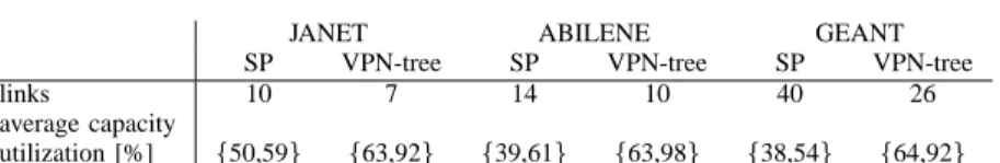
Table IV summarizes the average network resource uti-lization for the three example networks of Figure 4 using shortest-path as well as VPN-tree routing. The first row lists the number of links used by the two flow templates. The numbers {ul, un} represent the network-averaged utilization

of link capacities (ul) and node capacities (un), defined as the

percentage fraction of the mean capacities flowing over a link or through a node to the capacities that have to be provisioned to satisfy full traffic dynamism under the hose constraint. The numbers clearly reflect the better network utilization achieved by VPN-tree routing as compared to shortest-path routing. In addition, the number of links used by the VPN-tree template is smaller then used by the SP template.

D. MPLS and classes of service

So far, we only considered a single class of traffic, and demanded that the studied network architectures together with their associated flow templates should be able to accommodate the hose constraint for all ingress traffic. We now extend our analyses to the case of two traffic classes. We investigate the benefits of statistical multiplexing in IP/MPLS networks and study how this benefit relates to RLB and SRLB architectures. One of the main advantages of MPLS, and packet routing in general, is its ability to take advantage of statistical multiplex-ing to accommodate best-effort traffic. Thus, label-switched paths in MPLS represent ‘soft circuits’ in the sense that capacity that is currently unused for high priority (‘class A’) traffic may be used for lower priority (‘class B’) traffic. This way, the drawback of resource under-utilization, discussed in Section VI-C, is turned into an advantageous feature. To quantify the benefits of classes of service in IP/MPLS networks, we design an IP/MPLS network that guarantees a certain amount of class A traffic under the hose constraint. We then calculate the average amount of class B traffic that can be carried on top of this class A traffic by filling idle resources. These results are contrasted with the RLB network design, which by its very nature always utilizes all network resources to their full extent, and always provides guaranteed (class A) connectivity for the entire traffic.

Assuming the tight hose constraint (P

idij = D) for all

three networks of Figure 4, we partition the hose traffic D into class A hose traffic DA =αD and class B hose traffic

DB = (1−α)D. For each value of α, we dimension the

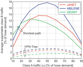
network to guarantee all possible class A demand matrices using the LP formulations described in Appendix XX. We then randomly generate ensembles of 1,000 class A matrices and route them on our networks. We record the link and node capacities used to route all class A demands. For each of the 1,000 class A matrices, we then generate 100 random class B matrices and greedily route as many class B demands as possible in random order, given the available capacities that are not used for the particular realization of class A traffic. We thus generate an ensemble of 100,000 random realizations of class B traffic that is permitted by the network, and take the average as our figure of merit. Figure 8 shows the average class B traffic supported by the network as a function of the amount of class A traffic α, both expressed as a percentage of the total hose trafficD. Solid curves apply to shortest-path routing, while dashed curves represent VPN-tree routing. As expected from our discussions on resource utilization, shortest-path routing allows for more class B traffic than VPN-tree routing, since it utilizes network resources to a smaller extent. Using VPN-tree routing, at most a few percent of the hose traffic can be routed as class B traffic, which demonstrates that the benefit of ‘soft’ circuits in combination with statistical multiplexing largely disappears for VPN-tree routing. For shortest-path routing, the studied IP/MPLS networks support up to 18% of the hose traffic as class B traffic, but also reject a significant amount of class B traffic. For example, designing the JANET network using shortest-path routing to support 50% of the node ingress traffic as class A traffic, the network allows for an additional 14% of the ingress traffic being sent as class B traffic, while 36% of the best-effort ingress traffic has to be dropped.

To design an RLB network that supports the same average traffic as the IP/MPLS network, we take the amount of class A

Class A traffic ( ) [% of hose demand]a

Average supportable class B traf fic [% of hose demand] 10 20 30 40 50 60 70 80 90 0 2 4 6 8 10 12 14 16 18 VPN-Tree Shortest-path JANET ABILENE GEANT

Fig. 8. Average class B traffic supported by the network as a function of class A trafficα, both expressed as a percentage of the total hose trafficD. Solid curves apply to shortest-path routing, dashed curves represent VPN-tree routing. The underlying networks are shown in Fig. 4.

(11)

TABLE IV

AVERAGE CAPACITY UTILIZATION.

JANET ABILENE GEANT

SP VPN-tree SP VPN-tree SP VPN-tree

links 10 7 14 10 40 26

average capacity

utilization [%] {50,59} {63,92} {39,61} {63,98} {38,54} {64,92}

traffic plus the average amount of class B traffic carried by the IP/MPLS network as the total ingress traffic to the RLB network. In the above numeric example for JANET, the result-ing RLB network therefore needs to support 50%+14%=64% of the hose traffic. This implies that in order to be cost-competitive, 64% of the cost of an RLB network needs to be lower than 50% of the cost of a multi-hop IP/MPLS network using shortest-path routing. Recalling the results from our cost analysis in Tables I – III, this indeed holds true for JANET: 64% of the cost of RLB on JANET is still 20% less expensive than multi-hop IP/MPLS using shortest-path routing.

E. The robustness premium

In this subsection we examine the following question: How much more capacity is needed to support all hose-constrained matrices (or any fixed universe of demand matrices) compared to just supporting a single benchmark demand matrix amongst them? We refer to the ratio of these link capacity costs as the robustness premium. The robustness premium obviously depends on the universe of demand matrices as well as on the choice of the benchmark matrix. Given that we are working with the class of hose matrices, it is natural to use as our benchmark matrix the product multicommodity flow matrix u where uij = DiDj/D ∀ i, j, and D = P_lDl.

(If all marginals are equal, this simplifies to the uniform multicommodity flow.)

The robustness premium naturally depends on the choice of a flow template since it determines how hops are transported in the physical layer. General robust network design problems actually treat the flow template as a variable in the optimization problem. Our study, however, focuses on a limited number of network architectures, which we can evaluate individually. In this subsection we present results on the robustness premium in terms of link costs only. Thus we effectively consider only three templates. The first is where every node pair routes their demand along a single shortest path. The second is where we are given the optimal VPN tree, and node pairs send flow on a simple path in the tree. We actually have two possible flow templates for trees (as discussed in Subsection IV-A – see Figure 2) but they are equivalent in terms of link cost. The last template considered is RLB.

Table V gives our empirical results for the robustness pre-mium on the three specific networks. We used the link capacity information developed in Section V and listed in Tables I – III. We have thus assumed that all ingress capacities are equal, and so we use the uniform demand matrix as our benchmark. Since we are dealing with uncapacitated networks, the cost of using randomized load balancing (RLB) is simply twice

TABLE V ROBUSTNESSPREMIUM

Flow Template JANET ABILENE GEANT

1. SP 2.48 2.46 2.46

2.VPN-Tree 1.66 1.50 1.31

3. RLB 2 2 2

that of satisfying this uniform demand. Note that the premium for using shortest-path routing is substantially more on all networks. Routing on an optimal VPN treeTopt significantly

reduces the required resources, consistent with [11], [22]. Moreover, the premium for using VPN trees decreases as network size increases.

Note that the robustness premium in Table V is based on link costs only. Accounting for node costs (according to Tables I – III) reveals that RLB, and in particular SRLB, is more advantageous than multi-hop routing using VPN-tree.

VII. CONCLUSIONS

We have seen that optimal VPN trees for hose matrices in uncapacitated networks can be used to support hub routing instead of direct routing. Since randomized load balancing (RLB) can be viewed as a convex combination of hub routing from different hubs, we propose selective randomized load balancing (SRLB) to achieve costs similar to optimal VPN trees, yet maintaining the benefits of RLB. We benchmarked SRLB as well as RLB against other single-hop, dual-hop and multi-hop circuit-switched and packet-switched network archi-tectures using shortest-path and VPN-tree routing. Using three representative carrier networks as examples, we investigated the cost structure of these architectures to support dynamically changing demand patterns for emerging flexible data services. Our analyses take into account the cost relationship between switching, routing, and transport equipment. Further work should incorporate more restrictions on the universe of valid matrices, such as in [2], [1], [20]. Work on the benefits of hierarchical (geographical) hubbing is also needed, as is a more thorough treatment of issues related to network resilience and restoration. Finally, it will be interesting to understand better the algorithmic issues in capacitated networks; this has already been addressed in [16].

APPENDIXA

In this appendix, we describe how we generated a set of randomly chosen demand matrices satisfying the hose constraint.

We sample the set D of all possible symmetric N ×N demand matrices[dij]associated with given capacities of the

(12)

network nodes Di ≥0, i= 1, . . . , N, N ≥4, more or less

uniformly using a standard M(arkov)C(hain)M(onte)C(arlo) algorithm. Recall thatd∈ Dis characterized by the conditions

dT =d≥0, dii= 0, n X j=1 dij =Di, i= 1, . . . , N. (2) Our MCMC algorithm starts with an arbitrary seed from D, and applies the following transition rule over and over: If d∈ D(c)is the current demand matrix, then we first choose randomly an index quadruple 1 ≤i < j < k < l≤N, and determine the maximal interval t∈[t0, t1]such that

d(t) :=d+t(Eij−Ejk+Ekl−Eli)∈ D. (3)

Here the matrices Eij (i 6= j) have exactly two non-zero

elements (more precisely, they are one at position ij andji), and their union forms a basis in the set of all symmetric matrices with zero diagonal. SinceEij−Ejk+Ekl−Elihas

always zero row sums, all updates given by (3) automatically satisfy the capacity constraints, andt0, t1 can easily be found

from the remaining constraintd(t)≥0:

t0=−min(dij, dkl), t1= min(djk, dli).

Then, choosingt randomly from the interval[t0, t1], we take

d(t) as the next demand matrix. Note that the transition rule requires a constant amount of computations, including calls to a standard random number generator.

It can be shown that, for any initial seed d0 ∈ D the

ensembles{d0, d1, . . . , dn}obtained by successively applying

the transition rule converge to a uniform distribution on D, as n→ ∞. Since experimentally good mixing was achieved for the ensemble sizes used in the simulations, we did not investigate the mixing time (generally, asN grows largernis required to achieve close to uniform sampling). Initial seeds can easily be determined for any set of feasible capacities by induction inN (the feasibility condition says that2 maxDi≤

P_D

i). For N = 2,3 and feasible capacities, or for N ≥ 4

and2 maxDi=PDi, the set Dconsists of one element.

APPENDIXB

We briefly outline the linear programs used to compute the link and nodal capacities required to support all demands under the hose model if we have some fixed single-path flow template f. For link capacities this is just the undirected version of LPs given in [9], [2], and so we focus on the LP for computing the maximum node switching capacity required. The following must be solved for each nodev in the network. Let Pv denote those paths P containing v as an internal

node, and with f(P) = 1. Note that even if f is a shortest path routing there may still be shortest paths containing v, but which are not contained in Pv. We create an auxiliary

directed graph G0 = (V, E0) as follows. The node set of G0 is the set of edge nodes (we have nominally been taking this to be all nodes) in the original physical network. For each P ∈ Pv between two edge nodes i and j, we add an

edge (i, j) to E0. (There may be several parallel edges if

the template has multiple paths between i, j but this has no impact on our computation.) The capacity of the switching fabric at v, required to support all hose demand matrices is equivalent to finding a maximum d-matching in G0 where d = (D1, D2, . . . , Dn). In other words, we seek a solution

to the following LP. MaximizeP

(i,j)∈E0xij subject tox≥0

and for each nodei6=v,P

jxij ≤DiandPjxji≤Di. Note

that edge(i, j)is distinct from(j, i)only because we chose to adopt the practice of treating traffic fromitojseparately from traffic fromjtoi. Though in implementation we have always computed equal and oppositely directed demands between any pair (that in addition use the same paths in opposite directions). Similarly, for link capacities we form the same LP, but instead it is based on using Pe, the set of paths P containing e and

withf(P) = 1.

ACKNOWLEDGEMENTS

We are grateful to Peter Oswald who implemented the pro-cedure for randomly generating demand matrices (Appendix A). We also thank Martin Zirngibl for valuable discussions.

REFERENCES

[1] A. Altin, E. Amaldi, B. Pelotti, M. Pinar, “Provisioning virtual private networks under traffic uncertainty”, Proc. of the International Network Optimization Conference INOC 2005; to appear Networks.

[2] D. Applegate and E. Cohen, “Making Intra-Domain Routing Robust to Changing and Uncertain Traffic Demands: Understanding Fundamental Tradeoffs,” Proc. ACM SIGCOMM 2003, 313-324 (2003).

[3] W. Ben-Ameur and H. Kerivin, “New economical virtual private net-works,” Commun. of the ACM 44(6), 69-73 (2003).

[4] W. Ben-Ameur and H. Kerivin, “Routing of Uncertain Demands,” to appear in Optimization and Engineering (2005).

[5] C.-S. Chang, D.-S. Lee, and Y.-S. Jou, “Load balanced Birkhoff-von Neumann switches, part I: one-stage buffering,” 2001 IEEE Workshop on High Performance Switching and Routing (HPSR) (2001). [6] C. Chekuri, G. Oriolo, M.G. Scutella, F.B. Shepherd, “Hardness of

Ro-bust Network Design”, Proc. of the International Network Optimization Conference INOC (2005); to appear Networks.

[7] N. G. Duffield, P. Goyal, A. Greenberg, P. Mishra, K. K. Ramakrishnan, and J. E. van der Merwe, “Resource management with hoses: Point-to-cloud services for virtual private networks,” IEEE/ACM Trans. on Networking 10(5), 679-692 (2002).

[8] F. Eisenbrand and F. Grandoni, “An improved approximation algorithm for virtual private network design,” Proc. 16th _{annual ACM-SIAM} Symposium On Discrete Algorithms (SODA) (2005).

[9] T. Erlebach and M. Ruegg, “Optimal bandwidth reservation in hose-model VPNs with multi-path routing,” IEEE INFOCOM 2004 (2004). [10] J. Andrew Fingerhut, Subhash Suri and Jonathan Turner, “Designing

Least-Cost Nonblocking Broadband Networks,” Journal of Algorithms, 287-309 (1997).

[11] A. Gupta, J. Kleinberg, A. Kumar, R. Rastogi, and B. Yener, “Pro-visioning a virtual private network: a network design problem for multicommodity flow,” ACM Symposium on Theory of Computing (STOC’01) (2001).

[12] A. Gupta, A. Kumar and T. Roughgarden, “Simpler and Better Approx-imation Algorithms for Network Design,” ACM Symposium on Theory of Computing (STOC’03) (2003).

[13] Cor A. J. Hurkens, J. C. M. Keijsper, Leen Stougie, “Virtual Private Network Design: A Proof of the Tree Routing Conjecture on Ring Networks”. IPCO 2005, 407-421, 2005.

[14] G. Italiano, S. Leonardi, and G. Oriolo,“Design of Networks in the Hose Model,” Proc. of ARACNE 2002, 65-76 (2002).

[15] I. Keslassy, S.-T. Chuang, K. Yu, D. Miller, M. Horowitz, O. Solgaard, and N. McKeown, “Scaling Internet Routers Using Optics,” ACM SIGCOMM 2003 (2003).

[16] M. Kodialam, T.V. Lakshman, and S Sengupta, “Efficient and Robust Routing of Highly Variable Traffic,” HotNets III (2004).

(13)

[17] T. Leighton and S. Rao, “An approximate max-flow min-cut theorem for uniform multicommodity flow problems with applications to approxima-tion algorithms”, in Proc. 29th IEEE Symp. on Foundaapproxima-tions of Computer Science (FOCS’88), 1988, pp. 422–431.

[18] D. Leung, W.D. Grover,Capacity Planning of Survivable Mesh-based Transport Networks under Demand Uncertainty, Photonic Network Comm. Springer, 10:2, pp123-140, 2005.

[19] D. Mitra, R.A Cieslak, “Randomized parallel communications on an extension of the omega network”, J. ACM, Vol.32, No.4 1987, 802-824. [20] H.Nagesh, V.Poosala, V.Kumar, P.J.Winzer, and M.Zirngibl, “Load-balanced architecture for dynamic traffic”, Optical Fiber Communication Conf. (OFC’05), Anaheim (CA/USA) OME67 (2005).

[21] H. Nagesh, V. Poosala, S. Sengupta, M. Alicherry, and V. Kumar, “NetSwitch: Load-balanced Data-over-Optical Architecture for Mesh Networks,” Lucent Technical Memorandum ITD-04-45867F (2004). [22] A. Kumar, R.Rastogi, A. Silberschatz, and B. Yener, “Algorithms for

provisioning virtual private networks in the hose model,” IEEE/ACM Trans. on Networking 10(4), 565-578 (2002).

[23] H. R¨acke, Minimizing Congestion in General Networks, Proceedings of the 43rd Symposium on Foundations of Computer Science 2002, 43–52. [24] S. Sengupta, V. Kumar, and D. Saha, “Switched optical backbone for cost-effective scalable core IP networks,” IEEE Comm. Magazine, June 2003, 60-70 (2003).

[25] L. G. Valiant, “A scheme for fast parallel communication”, SIAM J. Comput. 11(2), 350-361 (1982).

[26] I. Widjaja, A.I. Elwalid, “Exploiting parallelism to boost data-path rate in high-speed IP/MPLS networking, Workshop on High-Speed Networking 2002.

[27] P. J. Winzer, F. B. Shepherd, P. Oswald, and M. Zirngibl, “Robust Network Design and Selective Randomized Load Balancing,” accepted by the European Conference on Optical Communications (ECOC’05). [28] R. Zhang-Shen and N. McKeown, “Designing a Predictable Internet

Backbone Network”, HotNets III, San Diego, CA, (2004).

[29] ITU-T G.8081, “Definitions and terminology for automatically switched optical networks (ASON),” (2004).