lication in the following source:
Lee, Dong-Seop, Periaux, Jacques, Onate, Eugenio,
Gonzalez, Luis F.
,
& Qin, N. (2011) Active transonic aerofoil design optimization using robust
multiobjective evolutionary algorithms.
Journal of Aircraft
,
48
(3), pp.
1084-1094.
This file was downloaded from:
http://eprints.qut.edu.au/43952/
c
Copyright 2011 by the American Institute of Aeronautics and
As-tronautics, Inc.
Notice:
Changes introduced as a result of publishing processes such as
copy-editing and formatting may not be reflected in this document. For a
definitive version of this work, please refer to the published source:
Q1 Active Transonic Aerofoil Design Optimization Using
Multiobjective Evolutionary Algorithm Coupled
to Uncertainty Design Method
D. S. Lee
∗and J. Periaux
†International Center for Numerical Methods in Engineering, 08034 Barcelona, Spain
L. F. Gonzalez
‡Australian Research Centre Aerospace Automation, School of Engineering System, Queensland
University of Technology, Queensland 4009, Australia
and
E. Onate
§International Center for Numerical Methods in Engineering, 08034 Barcelona, Spain
DOI: 10.2514/1.C031237Q2 The use of adaptive wing/aerofoil designs is being considered, as they are promising techniques in aeronautic/ aerospace since they can reduce aircraft emissions and improve aerodynamic performance of manned or unmanned aircraft. This paper investigates the robust design and optimization for one type of adaptive techniques: activeflow control bump at transonicflow conditions on a natural laminarflow aerofoil. The concept of using shock control bump is to control supersonicflow on the suction/pressure side of natural laminarflow aerofoil that leads to delaying shock occurrence (weakening its strength) or boundary-layer separation. Such an activeflow control technique reduces total drag at transonic speeds due to reduction of wave drag. The location of boundary-layer transition can influence the position and structure of the supersonic shock on the suction/pressure side of aerofoil. The boundary-layer transition position is considered as an uncertainty design parameter in aerodynamic design due to the many factors, such as surface contamination or surface erosion. This paper studies the shock-control-bump shape design optimization using robust evolutionary algorithms with uncertainty in boundary-layer transition locations. The optimization method is based on a canonical evolution strategy and incorporates the concepts of hierarchical topology, parallel computing, and asynchronous evaluation. Two test cases are conducted: thefirst test assumes the boundary-layer transition position is at 45% of chord from the leading edge, and the second test considers robust design optimization for the shock control bump at the variability of boundary-layer transition positions. The numerical result shows that the optimization method coupled to uncertainty design techniques produces Pareto optimal shock-control-bump shapes, which have low sensitivity and high aerodynamic performance while having significant total drag reduction.
Q3
Nomenclature
c = chord
Cl = lift coefficient
Cp = pressure coefficient
CdTotal = total coefficient,CdViscousCdWave CdViscous = viscous drag coefficient
CdWave = wave drag coefficient
f = fitness functions
K = number of uncertainty step size
Re = Reynolds number
SCBH = height of shock control bump (%c)
SCBL = length of shock control bump (%c)
SCBP = peak position of shock control bump (%SCBL)
= angle of attack
I.
Introduction
I
NENGINEERING designs, it is inevitable to face uncertainty Q4design parameters that must be considered in an optimization task to produce a set of reliable optimal solutions (high performance and low sensitivity). Some of the design variables and system input parameters cannot be achieved exactly due to uncertainties in physical quantities such as manufacturing tolerances, material properties, and environmental conditions, including temperature, pressure, velocity, etc. In conventional design, these parameters are treated as a constant value with assumption. The design model obtained by conventional design methods has good performance at the standard design point; however, usingfixed/constant values for uncertain parameters makes a design modelfluctuate at offdesign conditions (high sensitivity: unstable) [1,2]. An alternative design Q5
strategy is the use of robust design when considering uncertainty design parameters to control the sensitivity and performance of the model [3,4]. In this paper, an activeflow control (AFC) device design is considered as a robust optimization application.
One of the important challenges in aeronautical engineering is to controlflow over the aerofoil/wing to reduce drag while increasing lift. One of the main reasons is that the drag reduction can save mission operating costs, condense critical aircraft emissions, and increase the performance envelope of the aircraft. Such drag reduction can be achieved by implementing a type of AFC called shock control bump (SCB) [5–8] without the need to design a new aerofoil or wing planform shape.
In this paper, a natural laminarflow (NLF) aerofoil, the Royal Aircraft Establishment (RAE)5243 (used as a baseline design), is Q6
investigated with SCB on the suction side to reduce total drag and to
Presented as Paper at the 49th AIAA Aerospace Sciences Meeting, Orlando, FL, 4–7 January 2011; received 14 September 2010; revision received 11 November 2010; accepted for publication 18 January 2011. Copyright © 2011 by the American Institute of Aeronautics and Astronautics, Inc. All rights reserved. Copies of this paper may be made for personal or internal use, on condition that the copier pay the $10.00 per-copy fee to the Copyright Clearance Center, Inc., 222 Rosewood Drive, Danvers, MA 01923; include the code and $10.00 in correspondence with the CCC.
∗Research Associate, UPC, Edificio C1, Gran Capitan. Member AIAA. †Professor, UPC, Edificio C1, Gran Capitan. Associate Fellow AIAA. ‡Lecturer, ARCAA, Queensland University of Technology. Member AIAA.
§Professor, UPC, Edificio C1, Gran Capitan.
extend its critical Mach and lift coefficients at high lift coefficient and transonicflow speeds. Two optimization test cases are conducted using advanced evolutionary algorithms (EAs) [9], and thefirst test considers a boundary-layer transition (BLT) (note that, in aero-dynamics, BLT is often used asxtr) position at 45% of chord. The second test is conducted with uncertainty design parameters, the variability of BLT positions, and lift coefficient values using a robust/ uncertainty design technique. In conventional design, aerofoil opti-mization is conducted at afixed/constant BLT position. However, BLT cannot be assumed as a constant value in a real design problem, especially for the AFC device design since the shape of AFC device will change the position of BLT. Therefore, the BLT location is considered as one of the uncertainty design parameters.
The paper will show how to control the design quality while considering uncertain design parameters, and it will demonstrate how to control the transonicflow on the current aerofoil using a SCB. The rest of the paper is organized as follows. Section II describes an optimization method and uncertainty design techniques. Aero-dynamic analysis tools are described in Sec. III. Section IV demonstrates the use of SCB. Section V considers SCB shape design optimization using single-objective and robust design approaches considering uncertain BLT positions. The overall results obtained in Sec. Vare discussed in Sec. VI. The paper concludes with a summary and some future research avenues in Sec. VII.
II.
Robust/Uncertainty Design Methods
The method couples hierarchical asynchronous parallel multi-objective EAs (HAPMOEAs) with an algorithm for SCB geometry, a module for robust design, and several aerodynamic analysis tools [9]. The algorithm is based on evolution strategies [10] and incorporates with the concepts of covariance matrix adaptation, distance-dependent mutation, hierarchical topology, asynchronous evaluation [11–15], and Pareto tournament selection that is applicable to single-objective or multisingle-objective problems [1,2]. The hierarchical topology can provide different models, including precise, inter-mediate, and approximate models. Each node belonging to the different hierarchical layer can be handled by a different EA code. HAPMOEA has also been coupled to uncertainty design techniques, as shown in [1,2,4]. Details and validation of HAPMOEA can be found in [9].
A. Robust/Uncertainty Design
A robust design method, also called the Taguchi method (uncertainty), pioneered by
Q7 Taguchi [3] in 1978, improves the quality of engineering productivity. An optimization problem can be defined as follows:
maximization or minimization
ffx1;. . .; xn; xn1;. . .; xm (1) where x1;. . .; xn represent design parameters and xn1;. . .; xm represent uncertainty parameters. The range of uncertainty design parameters can be defined by using two statistical functions: meanx
and variance [x x2] as part of the PDF.
The Taguchi optimization method minimizes the variability of the performance under uncertain operating conditions. Therefore, in order to perform an optimization with uncertainties, the fitness function(s) should be associated with two statistical formulas: the mean valuefand its variancefor standard deviationfpf:
f1 K XK i1 fi (2) f 1 K1 XK i1 fif2 (3)
where K denotes the number of subintervals of variation flow conditions.
The values obtained by the meanfand the variancefor standard deviationfrepresent the reliability of the model in terms of the magnitude of performance and stability/sensitivity at a set of uncertain design conditions.
B. Robust Design Method Implementation for Single-Objective Design Optimization Problems
The problem definition can be written with thefitness functions associated with a mean [Eq. (2)] and variance/standard deviation [Eq. (3)] as an uncertainty-based multiobjective design problem if a single-objective aerofoil design optimization problem considers a minimization of drag [fminCD] at a singleflight conditionMS. The robust designfitness functions are shown in Eqs. (4) and (5), while a singleflight condition becomes a set of uncertaintyflight conditions;M1K2 MS"; MS; MS"orM1andM1: CD 1 K XK i1 CDi (4) CD CD p 1 K1 XK i1 CDiCD 2 v u u t (5)
whereKrepresents the number of uncertainty conditions.
Consequently, the major role of the uncertainty technique is to improveCDquality with low drag coefficient and drag sensitivity at uncertainflight conditions by computing the mean and variance of criteria.
III.
Aerodynamic Analysis Tools
In this paper, the Eulerboundary-layer solver MSES, written by Drela [16], is used. The MSESsoftware is a coupled viscous/inviscid Q8
Euler method for the analysis and design of multielement/single-element airfoils. It is based on a streamline-based Euler discretization and a two-equation integral boundary-layer formulation, which are coupled through the displacement thickness and solved simulta-neously by a full Newton method. To obtain a prescribed lift coefficientCl, the angle of attackof the aerofoil is adapted. Details of MSES can be found in [16], and the validation of MSES compared with the wind-tunnel data can be found in [17].
IV.
Wave Drag Reduction via Active Flow
Control Bump
At transonic speed, theflow over the high camber wing causes shock waves where there is a large change of gas properties and the
flow becomes irreversible. Through the shock, total pressure decreases and entropy increases, which means an increase in the wave drag. Ashill et al. [5] proposed the concept of a transonic bump which so-called SCB by usinggeometry adaptation on an aerofoil. Q9
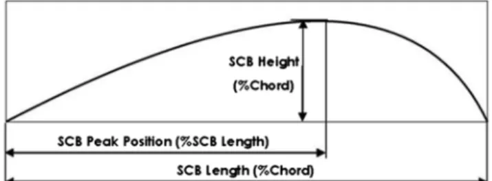
As illustrated in Fig. 1, the most common design variables for the SCB are lengthSCBL, heightSCBH, and peak positionSCBP, and the center of the SCB (i.e., 50% ofSCBL) is located where the shock occurs on the transonic aerofoil design.
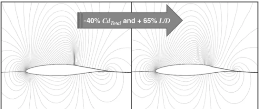
Figure 2 illustrates the concept and benefit of using SCB. The transonic flow over normal aerofoil without SCB accelerates to supersonic, and the pressure forms a strong shock that leads a high
CdWave; however, the pressure difference over the SCB causes the supersonicflow to decelerate to subsonic Mach numbers by a weaker shock wave, which leads to lower wave drag.
V.
Active Flow Control Bump (Shock Control Bump)
Design Optimization
The NLF aerofoil, RAE 5243 [6], is selected as a baseline design. The aerofoil has a maximum thickness of 0.14 at41%cfrom the leading edge and a maximum camber of 0.0186 at54:0%c. The baseline design is tested atflow conditionsM10:68,Cl0:82, andRe19:0106, with a BLT position at 45% of chord from the
leading edge. Figure 3 shows theCpcontours obtained by MSES. It can be seen that there is a strong normal shock on the suction side of the baseline design at45%cBLT position.
The shock occurs at 59.5% of chord, where a BLT position is at
45%c. This baseline design will be compared with the optimal SCB designed to minimize the total dragCdTotalin Secs. V.A and V.B.
A. Shock-Control-Bump Shape Design Optimization with Boundary-Layer Transition Position at 45%c
1. Problem Definition
This test case considers a single-objective SCB design opti-mization on the upper surface of the RAE 5243 aerofoil to minimize
the total drag atflow conditionsM10:68,Cl0:82, andRe
19:0106with BLT position at45%cfrom the leading edge. The fitness function is shown in Eq. (6):
fitness f minCdTotal minCdViscousCdWave (6)
2. Design Variables
The design variable bounds for the SCB geometry are illustrated in Table 1. The center of the SCB (50% of SCB length) will be located at the shock where theflow speed transits from supersonic to subsonic (60% of chord in this case). The SCB spans from approximately 45% of chord to 75% of chord if the SCB length is 30% of chord.
The maximum length of SCB is limited to30%cto prevent the SCB overflap and aileron control surfaces, which are usually located from75%cto trailing edge (100%c).
3. Implementation
The optimization was computed using HAPMOEA coupled to MSES using a single 42:8 GHz processor with the following details on multiresolution/population hierarchical populations [7]: Q10
1) Thefirst layer has a population size of 10 with a computational grid of36213points (node0).
2) The second layer has a population size of 20 with a computational grid of24131points (node1 and node2).
3) The third layer has a population size of 30 with a computational grid of36111points (node3 node6).
Note that the difference in accuracy between thefirst and the third layers is less than 5%.
4. Numerical Results
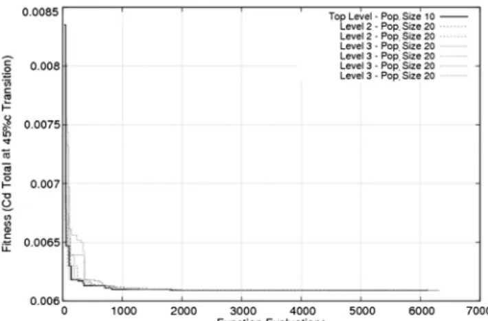
The algorithm was allowed to run for 24 h (as time stopping criterion) and for 6135 function evaluations. Convergence occurred after 1826 function evaluations (7.6 h), as shown in Fig. 4.
Fig. 2
Q30 Comparison of aerofoil without (left) and with SCB (right).
Fig. 3 Cpcontour obtained by RAE 5243.
Table 1 SCB design variables and bounds
Design variables Lower bound Upper bound
SCBL 0 30
SCBH 0 5
SCBP 0 100
aPeak position is in percentage of SCB lengthSCB
Table 2 compares the aerodynamic characteristics obtained by the baseline design (RAE 5243) and the baseline design with upper SCB. It can be seen that applying SCB on the upper surface of an RAE 5243 aerofoil reduces the wave drag by 95%, which leads to 40% of the total drag reduction. This optimal SCB improvesL=Dby 65%.
The design variables for the optimal SCB are shown in Table 3. Figure 5 compares the geometry of the baseline design and the baseline with optimal SCB. The baseline (RAE 5243) design with optimal SCB has a maximum thickness of 0.14 (t=cmax0:14) at
41%cfrom the leading edge, and the maximum camber is 0.0215 at
63:1%c. Adding the optimal SCB increases the maximum camber by 0.003, and the camber position moves toward to the trailing edge by
9%cwhile keeping the same maximum thickness as the baseline design.
Figure 6a shows theCpcontour obtained by the baseline design with optimal SCB. It can be seen that the strong shock on the baseline design shown in Fig. 3 is now 95% weaker by adding SCB. The pressure difference over the SCB causes the supersonic flow to decelerate to subsonic Mach numbers by a weaker shock wave, which is moved by7:0%ctoward the trailing edge, as shown in Fig. 6b.
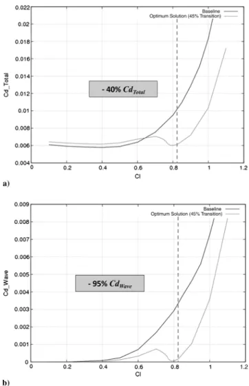
Figures 7a and 7b compare total drag CdTotal and wave drag
CdWavedistributions obtained by the baseline design and
Q11 one with the
optimal SCB along the Mach range; that is,M12 0:5:0:75with
ClFixed0:82, andRe19:0106with a BLT position at45%c.
The baseline design with SCB starts to produce lower total drag when the Mach number is higher than 0.67. By adding the optimal SCB, the baseline design reduces its total drag by 40% and its wave drag by 95% at the standardflight condition marked with the dashed line. The critical Mach number for baseline design (MC0:65) is extended to 0.68 due to the optimal SCB.
Figures 8a and 8b compare total drag distributions obtained by the baseline design and
Q12 one with the optimal SCB for aClrange; that is,
Cl2 0:1:1:1 with M10:68 and Re19:0106 with BLT
position at45%c. The baseline design with SCB starts to produce lower total drag when theClnumber is higher than 0.65. The critical
Clnumber for the baseline design (Clc0:5) is extended to 0.8 by applying optimal SCB on the suction side of baseline design.
Even though good results were obtained by using the single-objective design approach at the standard flow conditions, the optimal SCB produces an irregular/undesirableCdTotalfluctuation at
a range ofClfrom 0.6 to 0.82, as shown in Figs. 8a and 8b. This optimal solution is an overoptimized solution that does not perform well before reaching the standard flow/flight conditions. Such a
fluctuation should be treated as uncertainty in the design parameters, and the design engineer should take into account during the opti-mization. Therefore, it is necessary to use an uncertainty design technique to produce a set of solutions that have both low mean and sensitivity (nofluctuation: stable)CdTotalby considering variableCl Q13
values and BLT positions.
B. Robust Shock-Control-Bump Shape Design Optimization with Uncertainty in Boundary-Layer Transition Locations
1. Problem Definition
This test case considers a robust multiobjective SCB design optimization on the upper surface of the RAE 5243 aerofoil to minimize mean and standard deviation of total drag (CdTotal and CdTotal) at theflight conditionsM10:68andRe19:0106.
For uncertainty design parameters, twoCland three BLT positions are considered: that is, Cl 0:7; 0:82 and BLT 25%c; 37:5%c; 50%c. These can be statistically written as
BLT37:5%cand BLT12:5%c. The candidate SCB model will be evaluated at sixflight conditions (three BLT positions2Cl values), as shown in Table 4. Thefitness functions are shown in Eqs. (7) and (8), respectively:
Table 2 Aerodynamic characteristics obtained by single-objective design approach
Aerofoil CdTotal CdWave L=D
Baseline (RAE 5243) 0.01003 0.0032 81.72 with optimal SCB 0.00609 (40%) 0.00014 (95%) 134.56 (65%)
aC
lisfixed to 0.82.
Table 3
Q33 Optimal SCB design components
Variables SCB SCBL,%c 29.22 SCBH,%c 1.04 SCBP(%SCBL) 67.7 aPeak position SCBPis in percentage of SCB length;
and the optimal SCB is located betweenx0:4516,
y0:0858andx0:7440,y0:0475.
Fig. 5 Baseline design with optimal SCB at 45%cBLT (SO denotes single objective).
Fig. 6 Cpcontour: a)Cpdistribution and b) obtained by RAE 5243 with
f1minCdTotal 1 nm Xn i1 Xm j1 CdTotalij (7) f2minCdTotal 1 nm1 Xn i1 Xm j1 CdTotalijCdTotal2 v u u t (8)
where n and m represent the number of BLT positions and Cl conditions.
2. Design Variables
The design variable bounds for the SCB geometry were illustrated in Table 1. The center of the SCB (50% ofSCBL) will be located at the sonic point where theflow speed transits from supersonic to subsonic (58% of chord) at37:5%cBLT. The SCB will be located between43%cto73%cif SCB length is30%c.
3. Implementation
The optimization was computed using HAPMOEA coupled to MSES with the following details on multiresolution/population hierarchical populations [7]:
Q14
1) Thefirst layer has a population size of 15 with a computational grid of36213points (node0).
2) The second layer has a population size of 20 with a computational grid of24131points (node1 and node2).
3) The third layer has a population size of 40 with a computational grid of36111points (node3 node6).
Note that the difference in accuracy between thefirst and third layers is less than 5%.
4. Numerical Results
The algorithm was allowed to run for 50 h and 2450 function evaluations using a single42:8 GHzprocessor. Pareto optimal solutions are shown in Fig. 9, and their sensitivity and performance are compared with the baseline design and the optimal design from the single-objective approach (Sec. V.A). It can be seen that all Pareto members dominate the baseline for the second fitness function (standard deviation ofCdTotal:CdTotal), while Pareto members 1 to 9 Q15
dominate the baseline design in terms of mean and standard deviation ofCdTotal. Pareto members 1 to 3 dominate the optimal design from
Sec. V.A. Pareto members 1 and 3 are selected to compare aerodynamic performance with the baseline design and the optimal solution from Sec. V.A.
Table 5 compares the aerodynamic characteristics obtained by the baseline design (RAE 5243) and the baseline design with SCB obtained by Pareto members 1 and 3. It can be seen that applying the
Fig. 7 CdTotal: a) andCdWaveand b) Mach at 45%cBLT.
Fig. 8 CdTotal: a)CdWaveand b)Clat 45%cBLT.
Table 4 Variability offlight conditions (three BLT positions2Cl)
Variability Flight condition 1 Flight condition 2 Flight condition 3 Flight condition 4 Flight condition 5 Flight condition 6
BLT position,%c 25.0 25.0 37.5 37.5 50.0 50.0
optimal SCB obtained by Pareto member 1 on the suction side of the RAE 5243 aerofoil reduces the mean total drag by 24%. This optimal SCB improvesL=Dby 32.0%.
The mean and standard deviations obtained by the baseline design, single-objective, and robust Pareto members can be compared using cumulative the distribution function (CDF) and the probability density function (PDF). Figure 10a shows the CDF obtained by the baseline design, the optimal from the single-objective design (marked as SO optimal infigure), and the robust compromise Pareto solutions (marked as robust CS). It can be seen that all solutions obtained by single-objective and robust design methods have lower mean total drag when compared with the baseline design. Pareto member 1 reduces the mean total drag by 24% when compared with the baseline, while the optimal obtained by the single-objective approach reduces total drag by 17%. The standard deviation (sensitivity) can be represented by evaluating the gradient of the lines to the CDF value of 0.5 or 1 (steep gradientlow sensitivity). The PDF is plotted in Fig. 10b to have a clear sensitivity comparison between the baseline design and the single-objective robust design method. It can be seen that all solutions obtained by the single-objective and robust design methods have lower sensitivity (narrower and taller bell curve). Pareto member 3, obtained by the robust design method, has 41% total drag sensitivity reduction when compared with the baseline design, while the optimal obtained by the single-objective approach reduces total drag by only 11%. In other words, the robust design method has capabilities to produce a set of solutions that have better performance and sensitivity when compared with the single-objective optimization method.
For the detailed sensitivity analysis, the baseline design, the optimal solution obtained in Sec. V.A, and Pareto members 1 to 3 are selected and their CdTotal [Eq. (7)] and CdTotal [Eq. (8)] are recomputed at the variability of BLT37:49%c, BLT 0:0729%c25:0%c:50:0%c, and the variability of Cl0:761,
Cl0:0385, and0:7:0:82. In total, 500 nonuniformly distributed
flight conditions (50 BLT positions10Cl values) obtained by Latin hypercube sampling [18] are considered. Table 6 compares the aerodynamic characteristics obtained by the baseline design, the optimal solution obtained in Sec. V.A, and Pareto members 1–3. It can be seen that both optimal solutions produce lower total mean
drag and drag sensitivity with respect to 500 uncertain design conditions (BLT location and lift coefficient). Applying the optimal SCB obtained by Pareto member 1 produces 26% lower total drag while lowering the drag sensitivity by 22% when compared with the baseline design. The sensitivity obtained by the baseline design and all solutions is more than 2.5 times lower due to the increment of the number of uncertainty design conditions from 6 to 500. In addition, Fig. 11 compares mean and standard deviation using CDF and PDF.
One thing can be noticed is thatCdTotalandCdTotalbehaviors obtained by the CDF and PDF (shown in Fig. 10) considering six uncertainflight conditions are similar to theCdTotal andCdTotal
obtained by the CDF and PDF (shown in Fig. 11) considering 500
flight conditions between the baseline design and Pareto members 1 to 3. In other words, the simplified robust method with six uncertain
flight conditions still produces both lower total mean drag and drag sensitivity with respect to the variability of BLT positions and lift coefficient.
The design parameters of the SCB obtained by Pareto members 1– 3 are shown in Table 7. It can be seen that the length and height of SCB are reduced by approximately5%cand0:4%c, respectively, when compared with the optimal solution from Sec. V.A (Table 3). Figure 12 compares the geometry of the baseline design and the baseline with optimal SCBs. The baseline (RAE 5243) design with
Fig. 9 Pareto optimal front for robust SCB design at 45%cBLT. SO, CS, and PM represent the single-objective approach, compromised solutions, and Pareto members, respectively.
Table 5 Comparison offitness values obtained by robust design approach
Aerofoil CdTotal CdTotal L=D
Baseline 0.00935 0.00245 87.70
Optimal solution (Sec. V.A) 0.00780 (17%) 0.00219 (11%) 105.13 (20%) with Pareto member 1/SCB 0.00709 (24%) 0.00185 (24%) 115.66 (32%) with Pareto member 2/SCB 0.00728 (22%) 0.00158 (35%) 112.64 (28%) with Pareto member 3/SCB 0.00764 (18%) 0.00145 (41%) 107.33 (22%)
Fig. 10 Total drag comparison: a) mean using CDF and b) standard Q31 deviation (sensitivity) using PDF. SO and PM represent the single-objective approach and Pareto members, respectively.
SCB obtained by Pareto member 1 has a maximum thickness of 0.14 (t=cmax0:14) at 41%cfrom the leading edge and a maximum camber 0.0205 at62:5%c. Adding the SCB obtained by Pareto member 1 increases the maximum camber by 0.002, and its position is moved toward to the trailing edge by8:5%cwhile keeping the same maximum thickness as the baseline design.
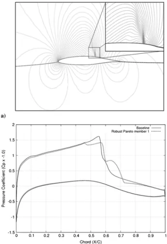
Figures 13a and 13b show the pressure contour and distribution obtained by the baseline design and Pareto member 1 at45%cBLT position. It can be seen that the strong shock on the baseline design shown in Fig. 3 is 77% weaker by adding SCB on the suction side. The SCB for Pareto member 1 reduces the total drag by 35% and improves the lift-to-drag ratio by 53%. In addition, the shock (Fig. 3) is now moved toward the trailing edge by2:0%c.
Figure 14a compares the total dragCdTotaldistributions obtained by the baseline design, the optimal solution obtained in Sec. V.A, and Pareto members 1–4. Theflight conditions areM12 0:6:0:72with
ClFixed0:82,Re19:0106, and the BLT position at45%c. It
can be seen that all solution obtained by the single-objective and robust design methods have lower total drag when the Mach number is higher than 0.67. The optimal solution from Sec. V.A produces lower total drag (40%) at Mach number 0.68, and Pareto members 1 and 4 reduce the total drag by 35 to 27%, respectively. Pareto member 1 has lower drag compared with other solutions when Mach is lower than 0.6775, while Pareto member 4 produces lower drag when Mach is higher than 0.685. The drag divergence Mach
Table 6 Comparison of mean and standard deviation of drag obtained by baseline design, single-objective optimal solution, and Pareto members 1 to 3, considering 500 uncertaintyflight conditions
Aerofoil CdTotal CdTotal L=D
Baseline 0. 00919 0.000893 83.31
Optimal solution (Sec. V.A) 0.00705 (23%) 0.000756 (15%) 109.59 (31%) Pareto member 1/SCB 0.00678 (26%) 0.000696 (22%) 113.17 (36%) Pareto member 2/SCB 0.00720 (22%) 0.000591 (34%) 106.38 (28%) Pareto member 3/SCB 0.00757 (18%) 0.000498 (44%) 100.93 (21%)
Fig. 11 Total drag comparison with 500 uncertaintyflight conditions: a) mean using CDF and b) standard deviation (sensitivity) using PDF.
Table 7 Pareto optimal SCB design components
Variables SCBL,%c SCBH.%c SCBP(%SCBL) Pareto member 1/SCB 25.93 0.76 69.3 Pareto member 2/SCB 27.12 0.85 76.2 Pareto member 3/SCB 26.45 0.75 81.3
aPeak position is in percentage of SCB length, and the Pareto member 1/SCB
starts from (x0:4490,y0:0859) to (x0:7083,y0:0540).
Fig. 12 Baseline design with optimal SCB at 45%cBLT.
Fig. 13 Cpcontour: a)Cpdistribution and b) obtained by RAE 5243
number for the baseline design (Mc0:66) is extended to 0.69 by applying the optimal SCB obtained by the single-objective and robust design methods.
Figure 14b compares total dragCdTotaldistributions at theflow conditionsCl2 0:1:1:1withMFixed0:68,Re19:0106, and
the BLT position at45%c. Even though the optimal solution obtained by the single-objective method produces lower total drag, Pareto members 1–4 have a stable total drag distribution at Cl range 0:6:0:82withoutfluctuation due to the stable wave drag. The drag divergenceClnumber for the baseline design (Clc0:5) is extended to 0.8–0.9 by applying the optimal SCB obtained by the single-objective and robust design methods.
Figure 14c compares wave dragCdWavedistributions obtained by the baseline design and single-objective and robust design methods. It can be seen that Pareto members 1–4 produce a stable wave drag when compared with the baseline design and the optimal solution obtained by the single-objective approach.
Figure 15a compares the total drag distributions at a range of Mach numbers; that is,M12 0:5:0:75withClFixed0:82,Re19:0
106, and the BLT position at25%c. The optimal solution obtained in
Sec. V.A and Pareto members 1–4 produce lower total drag compared with the baseline design when the Mach number is higher than 0.665. The optimal solution (Sec. V.A), Pareto members 1 and 4 reduce the total drag by 25, 24, and 23%, respectively, when compared with the
Fig. 14
Q32 Comparisons at 45%c BLT position. PM denotes Pareto member.
Fig. 15 Comparisons at 25%c BLT position. PM denotes Pareto member.
baseline design. Pareto member 1 has lower drag when Mach is lower than 0.6775, while Pareto member 4 has lower drag when Mach is lower than 0.685. The drag divergence Mach number for the baseline design (Mc0:66) is extended to 0.685 by applying the optimal SCB obtained by the single-objective and robust design methods.
Figure 15b compares total drag distributions at a range ofCl; that is,Cl2 0:1:1:1withMFixed0:68,Re19:0106, and the BLT
at25%c. The optimal solution from Sec. V.Afluctuates at the range ofCl 0:6:0:82, while Pareto members 1 and 4 have a stableCl distribution. The drag divergenceClnumber for the baseline design (Clc0:6) is extended to 0.8 by applying the optimal SCB obtained by the single-objective and robust design methods.
Figure 15c compares wave dragCdWavedistributions obtained by the baseline design and the single-objective and robust design methods. It can be clearly seen that Pareto members 1–4 produce stable wave drag when compared with the baseline design and single-objective approach. It should be noticed that the critical lift coefficient numbersClcfor the baseline design, the optimal solution obtained by the single-objective approach, and the Pareto members obtained by the robust design method are 0.3, 0.4, and 0.5, respectively.
The baseline design with the optimal SCB obtained by the single-objective and robust design methods are also tested at six normal
flight conditions, shown in Table 8.
The histogram shown in Fig. 16 compares the total drag obtained by the baseline design and the single-objective (Sec. V.A) and robust design approaches. It can be seen that the baseline design with the optimalSCB-robust 7 1 produces lower total drag when compared Q16
with the baseline design and the optimal SCB obtained by the single-objective method. The optimal SCB/Pareto member 1 reduces the total mean drag by 36% while lowering the total drag sensitivity by 77%. The optimal SCB obtained in Sec. V.A reduces the total mean drag and sensitivity by 9.5 and 48%, respectively, even though it produces higher drag atflight conditions 1, 3, and 5. Figure 17 compares the lift-to-drag ratio obtained by the baseline design, the optimal SCB from Sec. V.A, and Pareto member 1. It can be seen that Pareto member 1 has the biggest lift-to-drag improvement atflight condition 4. The pressure coefficient distributions at six flight conditions are shown in Figs. A1–A6, Sec. VII, and the Appendix.
One example (Cond4 from Fig. 17) is shown in Fig. 18, where the pressure contours obtained by the baseline design and Pareto member 1 are illustrated. Even though the SCB obtained by Pareto member 1 is optimized at the criticalflight condition, the optimal SCB/Pareto member 1 reduces the wave drag (CdWave0:0025) obtained by the baseline design by 99.5% (CdWave0:00001) and reduces the total drag by 40%, which leads to 65% improvement of
L=Dwhen compared with the baseline design.
To summarize the design test cases (Secs. V.A and V.B), the design engineer can choose one of the solutions (Pareto members 1 to 4) obtained by the robust multiobjective design optimization due to two main reasons. Thefirst is that, even though the optimal solution from Sec. V.A produces lower total drag at the standard/mean flight conditions (BLT position at45%c), Pareto members 1 to 4 have lower sensitivity (stable: nofluctuation) at the variability ofCland Q17
BLT positions25%c:50%c. In addition, it is clearly shown that
Table 8 Sixflight conditions
Conditions M1 Re Cl xTrans-Upper xTrans-Lower
Flight condition 1 0.69 11:7106 0.54 0.51 0.54 Flight condition 2 0.69 11:7106 0.69 0.51 0.54 Flight condition 3 0.70 11:7106 0.38 0.51 0.54 Flight condition 4 0.70 11:7106 0.50 0.51 0.54 Flight condition 5 0.73 11:7106 0.22 0.51 0.54 Flight condition 6 0.73 11:7106 0.34 0.51 0.54
Fig. 16 Drag reduction obtained by the baseline design, the single-objective solution, and robust Pareto member 1 (note that robust PM1 represents Pareto member 1 obtained by the robust design optimization, and Mean and STDEV represent the mean and standard deviation of
CdTotalat sixflight conditions).
Fig. 17 Drag reduction obtained by the baseline design, the single-objective solution, and robust Pareto member 1.
applying SCB obtained by the robust design method stabilizes the total drag of the baseline design at both normal and criticalflight conditions. The second is that Pareto members 1 to 4 have a smaller SCB than the optimal solution obtained by the single-objective method. In other words, the manufacturer can save material and weight costs, and fewer modifications are needed to the manu-facturing system.
VI.
Discussion
This paper explored the practical applications of MOEA with uncertainty for SCB shape optimization. The results from two test cases raise two discussion points and possible research avenues:
Q18
1) In this paper, a simplified robust design technique considering only six uncertainty flight conditions is used, and the obtained optimal solutions produce very similar statistical (CDF and PDF) behavior when compared with the CDF and PDF curves obtained by considering the 500 uncertaintyflight conditions. In other words, even though it is desirable to use a detailed robust design technique with more than 100 samplings for uncertainties conditions, this simplified robust method can be applied to a preliminary robust design optimization with low computational cost tofind a set of designs that have higher mean performance and lower sensitivity.
Q19 As
one of current research focuses on applying the concept of hierarchical asynchronous approach for not only using low/middle
flow solvers but also using detailed/intermediate/preliminary robust design methods to save a computational cost.
2) Thefirst discussion point on SCB design variation is that the algorithm considers only three control points,
Q20 which may require to
increase to perform a detailed design optimization. The second point is that the two test cases considered aerodynamic performance only, without any structural aspects. Even though SCB produces significant drag reduction, this can cause an unstable structure. The current work focuses on a multidisciplinary (aerostructure) design optimization implementation.
VII.
Conclusions
In this paper, the robust evolutionary optimization technique has been demonstrated, and a methodology for the design of adaptive wing/aerofoils that use AFC bump designs was developed. Analytical research shows the benefits of the coupling optimization method with robust design techniques to produce stable and high performance solutions. The use of SCB on an existing aerofoil can reduce significant transonic drag, which will save operating and manufacturing costs as well as emission reduction. Future work will focus on robust design optimization of SCB on a three-dimensional wing.
Appendix
Fig. A1 Cp distribution comparison atflight condition 1 (shown in
Table 8).
Fig. A2 Cp distribution comparison atflight condition 2 (shown in
Table 8).
Fig. A3 Cp distribution comparison atflight condition 3 (shown in
Table 8).
Fig. A4 Cp distribution comparison atflight condition 4 (shown in
Acknowledgments
The authors gratefully acknowledge E. J. Whitney and M. Sefrioui of Dassault Aviation for fruitful discussions on hierarchical evolutionary algorithms and their contribution to the optimization procedure. The
Q21 authors also acknowledge M. Drela at the Massachusetts Institute of Technology for providing MSES software. The authors are thankful to the organizers of the
Q22 database
workshop event“Integrated Multiphysics Simulation and Design Optimization: An Open Database Workshop for Multiphysics Software Validation”,¶ which took place at the University of
Jyvaskyla, Finland, 10–13 March 2010, igniting fruitful discussions on active flow control techniques (Chairman: N. Qin) in computationalfluid dynamics design with contributors to the bump test case problem.
References
[1] Lee, D. S., Gonzalez, L. F., Srinivas, K., and Periaux, J.,“Robust Evolutionary Algorithms for UAV/UCAV Aerodynamic and RCS Design Optimisation,”Computers and Fluids, Vol. 37, No. 5, 2008, pp. 547–564.
doi:10.1016/j.compfluid.2007.07.008
[2] Lee, D. S., Gonzalez, L. F., Srinivas, K., and Periaux, J.,“Robust
Design Optimisation Using Multi-Objective Evolutionary Algorithms,” Computers and Fluids, Vol. 37, No. 5, 2008, pp. 565–583.
doi:10.1016/j.compfluid.2007.07.011
[3] Taguchi, G., and Chowdhury, S.,Robust Engineering, McGraw–Hill, Q24
New York, 2000.
[4] Lee, D. S., Gonzalez, L. F., Periaux, J., and Srinivas, K.,“Evolutionary Optimisation Methods with Uncertainty for Modern Multidisciplinary Design in Aeronautical Engineering,” 100 Volumes of Notes on Numerical Fluid Mechanics: 40 Years Numerical Fluid Mechanics, Springer, Berlin, 2009, pp. 271–284.
[5] Ashill, P. R., Fulker, L. J., and Shires, A.,“A Novel Technique for Controlling Shock Strength of Laminar-Flow Aerofoil Sections,” Proceedings 1st European Forum on Laminar Flow Technology, Hamburg, Defence Research Agency, Farnborough, England, U.K., March 1992, pp. 175–183.
[6] Qin, N., Zhu, Y., and Shaw, S. T.,“Numerical Study of Active Shock Control for Transonic aerodynamics,” International Journal of Numerical Methods for Heat and Fluid Flow, Vol. 14, No. 4, 2004, pp. 444–466.
doi:10.1108/09615530410532240
[7] Wong, W. S., Qin, N., Sellars, N., Holden, H., and Babinsky, H.,“A Q25
Combined Experimental and Numerical Study of Flow Structures over Three-Dimensional Shock Control Bumps,”Aerospace Science and Technology, Vol. 12, No. 6, 2008, pp. 436–447.
doi:10.1016/j.ast.2007.10.011
[8] Qin, N., Wong, W. S., and LeMoigne, A.,“Three-Dimensional Contour Q26
Bumps for Transonic Wing Drag Reduction,” Proceedings of the Institution of Mechanical Engineers. Part G, Journal of Aerospace Engineering, Vol. 222, No. 5, 2008, pp. 619–629.
doi:10.1243/09544100JAERO333
[9] Lee, D. S., Gonzalez, L. F., and Whitney, E. J., Multi-Objective, Multidisciplinary Multi-Fidelity Design Tool: HAPMOEA: User Guide, Univ. of Sydney, Sydney, NSW, Australia, 2007.
[10] Hansen, N., and Ostermeier, A., “Completely Derandomized Self-Adaptation in Evolution Strategies,”Evolutionary Computation, Vol. 9, No. 2, 2001, pp. 159–195.
doi:10.1162/106365601750190398
[11] Koza, J., Genetic Programming II, Massachusetts Institute of Technology, Cambridge, MA, 1994.
[12] Michalewicz, Z.,Genetic AlgorithmsData StructuresEvolution Programs, Springer–Verlag, New York, 1992.
[13] Wakunda, J., and Zell, A.,“Median-Selection for Parallel Steady-State Evolution Strategies,”Parallel Problem Solving from Nature: PPSN VI, edited by M. Schoenauer, K. Deb, G. Rudolph, X. Yao, E. Lutton, J. Merelo, and H.-P. Schwefel, Springer, Berlin, 2000, pp. 405–414. [14] Van Veldhuizen, D. A., Zydallis, J. B., and Lamont, G. B.,
“Considerations in Engineering Parallel Multiobjective Evolutionary Algorithms,”IEEE Transactions on Evolutionary Computation, Vol. 7, No. 2, 2003, pp. 144–173.
doi:10.1109/TEVC.2003.810751
[15] Sefrioui, M., and Périaux, J.,“A Hierarchical Genetic Algorithm Using Multiple Models for Optimization,”Parallel Problem Solving from Nature, PPSN VI, edited by M. Schoenauer, K. Deb, G. Rudolph, X. Yao, E. Lutton, J. J. Merelo, and H.-P. Schwefel, Springer, New York, 2000, pp. 879–888.
[16] Drela, M., A User’s Guide to MSES 2.95, MIT Computational Q27
Aerospace Sciences Lab., Cambridge, MA, Sept. 1996.
[17] Lee, D. S., Periaux, J., Pons-Prats, J., Bugeda, G., and Onate, E., Q28
“Double Shock Control Bump Design Optimisation Using Hybridised Evolutionary Algorithms,” Special Session (S035–IEEE CEC): Evolutionary Computation in Aerospace Sciences, 2010 IEEE World Congress On Computational Intelligence (WCCI 2010), Barcelona, July 2010.
[18] Iman, R. L., Davenport, J. M., and Zigler, D. K.,Latin Hypercube Sampling (Program User’s Guide), Office of Scientific and Technical Information Rept. 5571631, Washington, D.C., 1980.
[19] Deb, K.,“Multi-Objective Genetic Algorithms: Problem Difficulties Q29
and Construction of Test Problems,”Evolutionary Computation, Vol. 7, No. 3, 1999, pp. 205–230.
doi:10.1162/evco.1999.7.3.205
Fig. A5 Cp distribution comparison atflight condition 5 (shown in
Table 8).
Fig. A6 Cp distribution comparison atflight condition 6 (shown in
Table 8).
¶Data available at http://jucri.jyu.fi[retrieved ].
Queries
IMPORTANT: PLEASE READ CAREFULLY.
When production of AIAA journal papers begins, the official approved PDF is considered the authoritative manuscript. Authors are asked to submit sourcefiles that match the PDF exactly, to ensure that thefinal published article is the version that was reviewed and accepted by the associate editor. Once a paper has been accepted, any substantial corrections or changes must be approved by the associate editor before they can be incorporated.
If you and the EIC settled on somefinal changes to your manuscript after it was accepted, it is possible that your page proofs do not reflect thesefinal changes. If that is the case, please submit these changes as itemized corrections to the proofs.
Iffinal changes were made to thefigures, please check thefigures appearing in the proofs carefully. While it is usual procedure to use thefigures that exist in the sourcefile, if discrepancies are found betweenfigures (manuscript sourcefile vs the approved PDF), thefigures from the PDF are inserted in the page proofs, again deferring to the PDF as the authoritative manuscript. If youfind that agreed-uponfinal changes to yourfigures are not appearing in your page proofs, please let us know immediately.
Q1. The 14-word title currently exceeds the 12-word limit by AIAA. Please reduce its length. Please note that acronyms are not allowed in the title.
Q2. Please check that the above copyright (©) type is correct.
Q3. Definitions of acronyms have been moved from the nomenclature into the text of the article, per AIAA style. Q4. Major syntax adjustments were made throughout; please read closely to confirm that your meaning was retained. Q5. Please clarify“high sensitivity: unstable”, as complete sentences/phrases are required by AIAA.
Q6. We have defined RAE as Royal Aircraft Establishment. Is this correct?
Q7. The text reads“Taguchi [3] in 1978...”, but the reference was written by Taguchi and Chowdhury in 2000. To comply with AIAA guidelines, please provide a reference to match the text or change the text to read“In 1978, the Taguchi method...”
Q8. Please supply a definition for MSES.
Q9. “which so-called SCB by using”is unclear. Please review and edit as necessary.
Q10. The numbered items were edited to be complete sentences, per journal guidelines. Please check that your meaning was retained. Q11. Please clarify what“one”refers to.
Q12. Please clarify what“one”refers to.
Q13. Please clarify“nofluctuation: stable”, as AIAA requires complete sentences/phrases.
Q14. The numbered items were edited to be complete sentences, per journal guidelines. Please check that your meaning was retained. Q15. Does the colon betweenCdTotalandCdTotalrepresent a ratio? If not, please clarify.
Q16. Please clarify/define“SCB-robust 7 1”.
Q17. Please clarify“stable: nofluctuation”, as AIAA requires complete sentences/phrases.
Q18. The numbered items have been edited to be complete sentence, per journal guidelines. Please check that your meaning was retained.
Q19. The sentence begninng,“As one of current research focuses...”is unclear/incomplete. Please review and edit as necessary. Q20. “which may require to increase to perform”is unclear. Please review and edit as necessary.
Q21. MIT has been defined as Massachusetts Institute of Technology and CFD as computationalfluid dynamics. Is this correct? Q22. Please note that the Acknowledgments section must be contained in one paragraph.
Q23. Please provide the date of retrieval for http://jucri.jyu.fi. Also, it is unclear what how the url is related to the text. Please provide a more specific url or clarify in the text.
Q24. Please provide the page numbers used for Refs. [3, 11, 12, 16]. Q25. The issue has been added for Ref. [7]. Please confirm this is correct.
Q26. A check of online databases revealed a possible error in Ref. [8]. The pages have been changed from’605–617’to’619–629’. Please confirm this is correct.
Q27. The references have been reordered so that they are cited in the text in numerical order.
Q28. If Ref. [17] is a published proceedings, please provide the name and location of the publisher (not of the conference host) and the page numbers used. If it is a conference paper, please provide the paper number and the organizer’s name. If it is a CD-ROM, please provide the name and location of the CD-ROM producer.
Q29. Reference 19 was not cited in text. Please cite the reference in text in numerical order or remove the reference.
Q30. AIAA has not indicated color use for your paper. Please confirm that your paper should be grayscale and that allfigures are satisfactory. If any replacementfigures are needed, please send them in .eps or .tiff format to [email protected] and use code C031237 in the subject line. Formats of .jpg, .doc, or .pdf can be used with some loss of quality.
Q31. The captions for Figs. 10 and 11 have been edited to have overall captions, per journal guidelines. Please check that your meaning is retained.
Q32. The caption of Fig. 14 was edited to be an overall caption, as it is against journal style to repeat the information in the subcaptions in the main caption.