Vortex Generators in a Two-Dimensional, External-Compression Supersonic Inlet
Ezgihan Baydar1 and Frank K. Lu2
University of Texas at Arlington, Arlington, Texas 76019
and John W. Slater3
NASA Glenn Research Center, Cleveland, OH 44135
Vortex generators within a two-dimensional, external-compression supersonic inlet for Mach 1.6 were investigated to determine their ability to increase total pressure recovery, reduce total pressure distortion, and improve the boundary layer. The vortex generators studied included vanes and ramps. The geometric factors of the vortex generators studied included height, length, spacing, and positions upstream and downstream of the inlet terminal shock. The flow through the inlet was simulated through the computational solution of the steady-state Reynolds-averaged Navier-Stokes equations on multi-block, structured grids. The vortex generators were simulated by either gridding the geometry of the vortex generators or modeling the vortices generated by the vortex generators. The inlet performance was characterized by the inlet total pressure recovery, total pressure distortion, and incompressible shape factor of the boundary-layer at the engine face. The results suggested that downstream vanes reduced the distortion and improved the boundary layer. The height of the vortex generators had the greatest effect of the geometric factors.
Nomenclature
AIP = aerodynamic interface plane ARvg = aspect ratio of the vortex generator
αvg = slope of the ramp-type vortex generator
bvg = length of the base of the ramp
DPC/P2 = circumferential total pressure distortion descriptors
DPR/P2 = radial total pressure distortion descriptors
DS = downstream of inlet terminal shock
hvg = vortex generator height
𝐻𝑖 = incompressible shape factor, 𝛿𝑖∗⁄𝜃𝑖
Lvg = length
M = Mach number
Nvg = number of devices
p = pressure
svg = spanwise VG spacing
vg = characteristic angle for the vortex generator u = streamwise velocity (x-direction)
𝑢𝑑𝑖𝑓𝑓 = streamwise velocity difference, 𝑢 − 𝑢𝑏𝑎𝑠𝑒𝑙𝑖𝑛𝑒
u0 = incoming freestream velocity US = upstream of the inlet terminal shock VGs = vortex generators
W = flow rate
x, y, z = Cartesian coordinates
𝛿 = boundary-layer thickness, 99% of local 𝑢𝑚𝑎𝑥
1 NASA Harriett G. Jenkins Fellow, Aerodynamics Research Center, Mechanical and Aerospace Engineering Department, Box 19018, AIAA Student Member.
2 Professor and Director, Aerodynamics Research Center, Mechanical and Aerospace Engineering Department, Box 19018, AIAA Associate Fellow.
3 Aerospace Engineer, Inlets and Nozzles Branch, MS 5–12, 21000 Brookpark Road, AIAA Senior Member.
𝛿𝑖∗ = incompressible displacement thickness, ∫ (1 − 𝑢/𝑢0𝛿 ∞)𝑑𝑦 𝜃𝑖 = incompressible momentum thickness, ∫ 𝑢/𝑢0𝛿 ∞(1 − 𝑢/𝑢∞)𝑑𝑦 Subscripts
0 = freestream flow conditions 2 = AIP flow conditions cap = reference capture condition
I. Introduction
An external-compression, supersonic inlet has an external supersonic diffuser that generates an external shock system that decelerates and compresses the flow being captured by the inlet [1]. The external shock system ends with a terminal shock that decelerates the captured inlet flow from supersonic to subsonic conditions and is external to the interior ducting of the inlet. The terminal shock can be either a normal shock or a strong oblique shock. Downstream of the terminal shock, the captured inlet flow enters the internal ducting of the inlet consisting of a throat section and subsonic diffuser. The subsonic diffuser has the engine-face at its downstream end. The aircraft of interest here have turbo-fan engines with a circular engine face and a spinner about the engine axis.
Recent studies have proposed streamline-traced, external-compression (STEX) inlets for aircraft speeds of about Mach 1.6 [2-4]. A STEX inlet has an external supersonic diffuser obtained from tracing streamlines through an axisymmetric, inward-turning parent flowfield containing a strong, oblique shock that forms the terminal shock. The STEX inlets have the positive characteristics of lower wave drag and lower external disturbances that contribute to sonic boom than that of traditional axisymmetric and two-dimensional inlets. A negative characteristic of STEX inlets is the interaction of the terminal shock with the turbulent boundary layer generated by the external supersonic diffuser. This interaction generates a region of low-momentum flow in the subsonic diffuser that may result in separated and unsteady flow. The resulting total pressure losses and total pressure distortion at the engine face reduce inlet efficiency and create possible conditions for instability within the turbo-fan engine. The STEX inlet showed about 3-percent lower total pressure recovery and higher engine-face distortion than a similar axisymmetric spike inlet [4].
One approach for reducing total pressure losses and distortion due to the terminal shock/boundary layer interaction is to incorporate flow control within the inlet. The approach of this paper was to use flow control devices that generated vortices that energized the flow within the boundary layer. The devices are known as vortex generators (VGs) and the types of devices studied here included rectangular vanes and ramps shaped as a right-angle pyramids. The study explored the effect of the height, length, and spacing of the devices. Also studied was the placement of the VGs upstream or downstream of the terminal shock/boundary-layer interaction.
To simplify the study of the effects of VGs for reducing the adverse effects of normal-shock/turbulent boundary-layer interactions, a two-dimensional, external-compression inlet was designed to represent the flowfield of the STEX inlet. The external supersonic diffuser of the two-dimensional inlet consisted of a series of ramps rather than a three-dimensional, streamline-traced surface. The terminal shock was a normal shock rather than a strong oblique shock of the STEX inlet. Downstream of the terminal shock/boundary-layer interaction and within the throat section, the inlet surface was a flat surface rather than a three-dimensional surface of the STEX inlet. This greatly simplified the geometry modeling and grid generation of the flow control devices as they were resized and re-positioned on the inlet surfaces. The key interaction of the boundary layer and the terminal shock was represented as well as the development of a low-momentum or separated region downstream of the terminal shock.
The paper is organized as follows. Section II discusses the geometry and flow features of the external-compression supersonic inlet studied in this work. Section III discusses the computational fluid dynamics (CFD) methods used to solve the steady-state, Reynolds-averaged Navier-Stokes (RANS) equations for the simulation of the aerodynamics of the inlet flowfields. Section IV discusses the vane and ramp-type vortex generators. Section V discusses the baseline inlet flowfield without vortex generators. Section VI presents the results for the inlet performance as obtained from the computational simulations.
II. External-Compression Inlet
The two-dimensional, external-compression inlet was designed using the same conditions as the streamline-traced, external-compression (STEX) inlet [2]. The freestream was a Mach number of 1.6 with conditions of the standard atmosphere at an altitude of 40,000 feet. The engine face had a diameter of 3.0 feet with an elliptical spinner with a hub-to-tip ratio of 0.3 and aspect ratio of 2.0. The engine corrected flow rate corresponded to a mass-averaged Mach
number of 0.52 at the engine face. The design of the inlet and the generation of the geometry was performed using the SUPIN (Supersonic Inlet Design and Analysis) tool [5-6]. SUPIN uses the freestream and engine-face conditions along with a small set of design factors to size the inlet, compute the inlet performance, and create the inlet geometry.
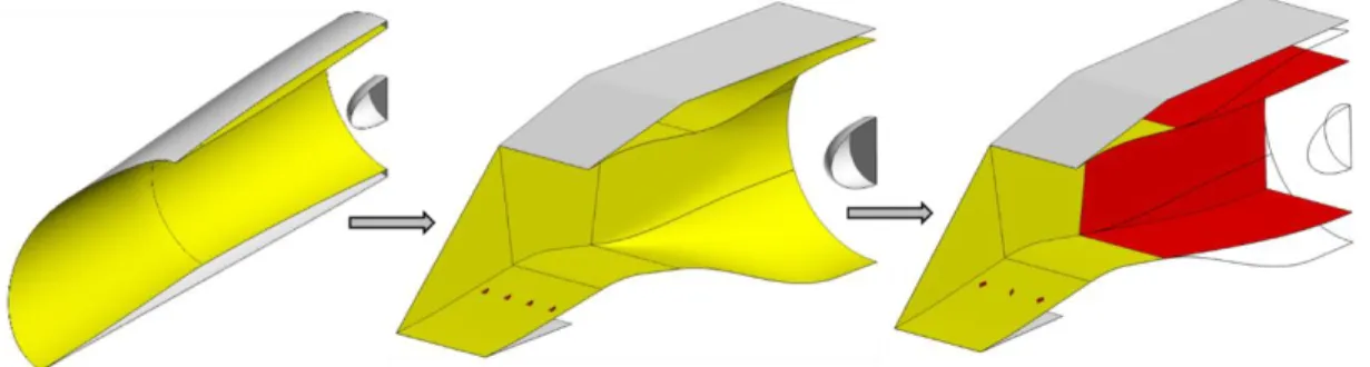
The parent flowfield for the STEX inlet was established with a Mach 1.6 inflow and a Mach 0.9 outflow. The angle of the leading edge was −5.0 degrees. The parent flowfield contained a weak oblique shock as the leading wave followed by an isentropic supersonic compression which ended with a strong oblique shock that decelerated the flow to Mach 0.9 and turned the flow into the axial direction. The surface of the external supersonic diffuser was created by streamline-tracing upstream through the parent flowfield starting from a circular tracing curve at the throat. The circular tracing curve was offset from the axis-of-symmetry of the parent flowfield to result in a scarfed leading edge for the external supersonic diffuser. The subsonic diffuser was created to be axisymmetric about the inlet axis and with length that imposed an equivalent conical angle of 3.0 degrees. The STEX inlet had a capture area of Acap = 5.979 ft2, inlet length of Linlet = 8.507 feet, and an inlet total pressure recovery of pt2/pt0 = 0.969. The left image of Fig. 1 shows the STEX inlet.
The two-dimensional, external-compression inlet was designed using SUPIN with a three-stage, external supersonic diffuser. The first stage was a ramp with an angle of 5.0 degrees. The second stage was an isentropic contour that decelerated the flow to Mach 1.3 with a turning of 3.653 degrees. The third stage was a ramp of the same angle as the end of the second stage. The normal terminal shock was positioned at station 1. The throat section involved a turning of 11.653 degrees to form an aft ramp with an angle of -3.0 degrees. Downstream of the terminal shock, the cross-sectional area of the throat section gradually increased. The subsonic diffuser had a length of 3.742 feet and involved a transition from a rectangular section at the start of the subsonic diffuser to a circular cross-section at the engine face. The capture area was Acap = 5.982 square-feet and the inlet length was Linlet = 7.757 feet. The inlet total pressure recovery estimated by SUPIN was pt2/pt0 = 0.9695. The middle image of Fig. 1 shows the two-dimensional inlet.
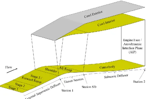
The two-dimensional inlet was simplified to focus just on the terminal-shock/boundary-layer interaction and the formation of the low-momentum region downstream of the terminal shock. The original subsonic diffuser was replaced by a duct with a rectangular cross-section throughout the length of the subsonic diffuser. The width of the duct was constant through the subsonic diffuser and set equal to the diameter of the engine face. Figure 1 shows this simplification with the red-colored rectangular duct. Figure 2 shows the simplified two-dimensional inlet with the parts and stations identified. The external supersonic diffuser is shown with the three stages. Ramp 3 is also referred to as the forward ramp and was modeled as a flat, rectangular plane. The throat section consists of the shoulder over which the flow turns and the aft ramp, which was modeled as a flat, rectangular plane. Station SD is the end of the aft ramp and the start of the subsonic diffuser. Station 2 is the end of the subsonic diffuser at the engine face, which was modeled as a flat rectangle with no spinner. Station 2 is also the location of the aerodynamic interface plane (AIP) where the inlet total pressure recovery and distortion are evaluated.
To further simplify the flowfield, the planar sidewalls of the inlet were assumed to be inviscid so as not to create boundary layers along those surfaces. An inviscid wall was placed at the inlet symmetry boundary, which made the width of the modified inlet equal to half of the engine-face diameter. The use of inviscid walls avoided the possible creation of vortices and boundary-layer separation at the right-angle corners of the inlet. The neglect of corner effects is based on the fact that the STEX inlet does not contain such corner flows. Thus, the modified two-dimensional inlet flowfield is not a realistic flowfield; however, the flowfield captures the important interaction of the normal, terminal shock with the turbulent boundary layer and the creation of the low-momentum region.
Figure 2. Parts and stations of the two-dimensional, rectangular inlet. III. CFD Analysis Methods
The methods of computational fluid dynamics (CFD) provided analysis of the aerodynamics of the turbulent flow through the two-dimensional inlet. The Wind-US CFD code was used to solve the steady-state, Reynolds-Averaged Navier-Stokes (RANS) equations for flow properties on a multi-block, structured grid within the flow domain about the inlet [7]. The CFD solutions also allowed visualization of the flowfield to better understand the shock structures, boundary layers, and other flow features within and about the inlet. From the flowfield, the inlet performance properties were obtained.
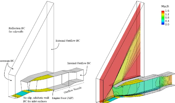
Figure 3 shows the flow domain and boundary conditions used for the CFD simulations. The internal and external surfaces of the inlet formed a portion of the boundary of the flow domain where adiabatic viscous wall boundary conditions were imposed. The right image of Fig. 3 shows Mach number contours on a vertical plane for an example flowfield. The geometry and boundary conditions of the inlet are planar, and so, the plane shown in Fig. 3 represents the flow throughout the width of the flowfield. The flow domain had inflow boundaries upstream and about the inlet where freestream boundary conditions were imposed. The incoming freestream flow had a Mach number of M0 = 1.6. The freestream thermodynamic state (p0,T0) corresponded to conditions of the standard atmosphere with an altitude of h0 = 40,000 feet. An oblique shock was formed at the leading edge of the first stage of the external supersonic diffuser and intersected the cowl lip. A short isentropic section of the second stage further compresses and decelerates the flow to Mach 1.3 over the third stage. The normal terminal shock is positioned at the cowl lip plane and is approximately normal to the third stage (forward ramp). On the cowl exterior, an oblique shock is formed at the cowl lip followed by an expansion as the cowl exterior becomes horizontal. At the end of the cowl exterior, the domain had an outflow boundary where supersonic extrapolation boundary conditions were imposed. Within the throat section, the flow was turned past the shoulder and was further diffused in the subsonic diffuser. Downstream of the engine face, a converging-diverging nozzle section was added to the flow domain to set the flow rate within the inlet. The nozzle throat was set to be choked so that the internal outflow of the nozzle was supersonic. This allowed a non-reflective extrapolation boundary condition to be imposed. This approach minimizes adverse effects of the internal outflow boundary condition on the flow at the engine face.
The multi-block, structured grids were generated for the flow domain using SUPIN. The inlet with no vortex generators had a grid consisting of twenty-four blocks. SUPIN used inputs for the grid spacing normal to the wall, streamwise grid spacing within the throat section, and grid spacing in the cross-stream direction to automatically establish the number of grid points along the edges and surfaces of the inlet and within the flow domain. In addition, SUPIN created the boundary condition file for the Wind-US CFD code.
Wind-US used a cell-vertex, finite-volume representation for which the flow solution was located at the grid points. In Wind-US, the RANS equations were solved using an implicit time-marching algorithm with a first-order, implicit Euler method using local time-stepping. The flowfield was initialized at all grid points with the freestream flow conditions. Local time-stepping was used within the marching time steps to converge the flow solution to the
steady-state flowfield. The temperatures allowed the use of the ideally-perfect air model. The inviscid fluxes of the RANS equations were modeled using a second-order, upwind Roe flux-difference splitting method. The flow was assumed to be fully turbulent with the turbulent eddy viscosity calculated using the two-equation Menter shear-stress transport (SST) model [8].
Figure 3. Flow domain, boundary conditions, and example flow solution. IV. Baseline Inlet Flowfield
The baseline inlet flowfield is the flow through the inlet without any vortex generators. This section discusses the inlet performance metrics that characterize the inlet flow and presents the performance for the baseline inlet flowfield. Included is a discussion of the variation of the inlet performance metrics with refinement of the computational grid.
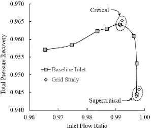
The first metric of inlet performance is the inlet flow ratio, which is defined as the rate of flow passing through the engine face divided by the reference capture flow rate (W2/Wcap). The inlet flow rate (W2) is computed as an average of the flow computed through grid planes through the outflow nozzle section. The reference capture flow rate (Wcap) is computed as the flow at the freestream conditions passing through the reference capture area (Acap). The inlet flow rate is controlled by the area of the throat of the outflow nozzle. At the critical inlet flow rate, the inlet flow rate is equal to the reference capture flow rate (W2 = Wcap) and the terminal shock is located at the cowl lip plane. The top image of Fig. 4 shows the Mach number contours on a vertical plane for the inlet flowfield near the critical operating condition. The interaction of the terminal shock with the boundary layer of the external supersonic diffuser creates a low-momentum region along the centerbody through the throat section and subsonic diffuser. For the critical operating condition, there is very little boundary-layer separation on the lower surfaces of the throat and centerbody.
At supersonic freestream conditions, the inlet flow rate cannot exceed the reference capture flow. Thus, increasing the nozzle throat area beyond that for the critical flow condition will only draw the terminal shock into the inlet to create a supercritical condition. The bottom image of Fig. 4 shows the inlet at a supercritical operating condition. For the supercritical operating condition, a pocket of higher Mach number flow developed on the shoulder. This resulted in a larger region of boundary-layer separation on the lower surfaces.
Reducing the nozzle throat area below that for the critical flow condition will reduce the inlet flow rate and increase the back-pressure in the subsonic diffuser to create a subcritical condition. This pushes the terminal shock forward of the cowl lip so that the excess flow can be spilled past the cowl lip.
The second metric of inlet performance is the inlet total pressure recovery, which is defined as the mass-averaged total pressure at the AIP divided by the freestream total pressure (pt2/pt0). The inlet total pressure at the AIP (pt2) is computed from the flowfield on the computational grid at the AIP.
The variation of the inlet total pressure recovery with the inlet flow ratio is inlet characteristic curve, which is also known as the “cane” curve. Figure 5 shows the characteristic curve for the baseline inlet. The segment of the curve for the supercritical conditions should be a vertical line, which indicates a constant inlet flow ratio. The points labeled “Supercritical” in Fig. 5 are represented by the bottom image of Fig. 4. The points labeled “Critical” in Fig. 5 are represented by the top image of Fig. 4 and are slightly subcritical with about 1% spillage of the flow past the cowl lip. The segment of the curve for the subcritical conditions indicate gradually lower inlet flow ratios as more flow is spilled past the cowl lip.
Figure 5. Characteristic curve for the baseline inlet.
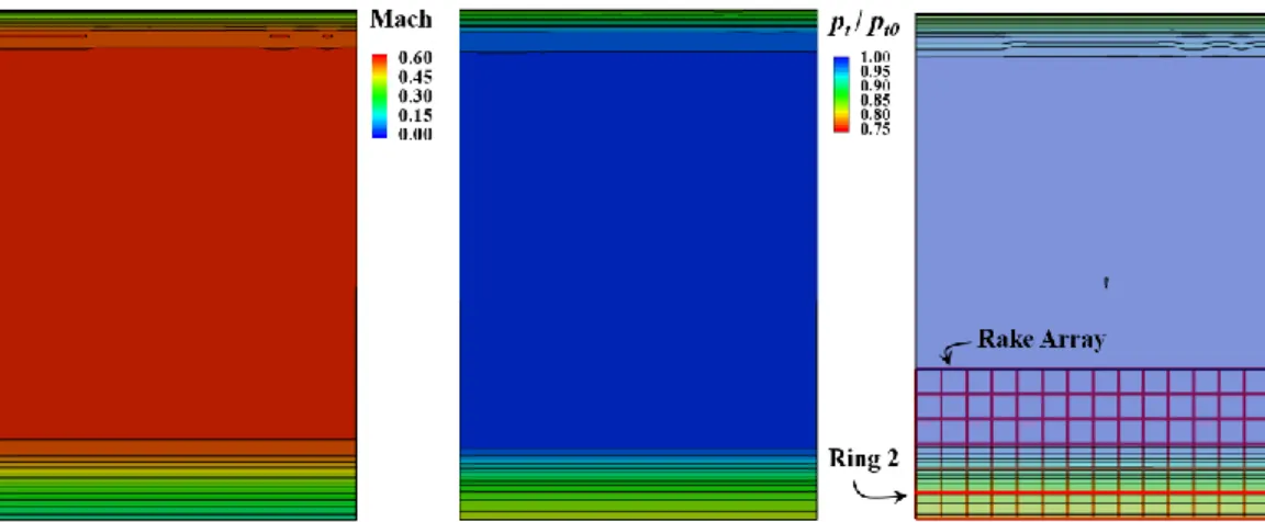
The third metric of the inlet performance is the shape of the boundary layer along the centerbody at the AIP as represented by the incompressible shape factor (Hi). The left image of Fig. 6 shows the Mach number contours at the AIP with the boundary layers at the bottom and top of the AIP. Since the baseline inlet flow is two-dimensional, the boundary layer is uniform across the crosswise span of the inlet at the AIP. The boundary layer at the bottom is larger due to the low-momentum region created along the centerbody. The incompressible shape factor for the AIP was computed as the area-average of the values for the boundary-layer profiles at each of the vertical grid lines that traverse the boundary layer across the span of the inlet.
Figure 4. Mach number contours on a streamwise plane for the critical (top) and a supercritical (bottom) CFD simulations of the baseline inlet.
The fourth and fifth metrics of inlet performance are descriptors of the “circumferential” and “radial” total pressure distortion at the AIP. The terms “circumferential” and “radial” are in quotes because this terminology and the methods for computing these distortion descriptors were based on those of the SAE Aerospace Recommended Practices (ARP) 1420 document [9]. The center image of Fig. 6 shows the total pressure contours at the AIP normalized by the freestream total pressure. Here, the AIP was rectangular, so the circumferential direction corresponds to the cross-stream direction and the radial direction corresponds to the vertical direction. A rectangular rake array with seven “rings” or horizontal members and fifteen “rakes” or vertical members was used. The right image of Fig 6 shows the rectangular rake array. The CFD solution was interpolated onto the “probes” of the rake array, which were at the intersection of the ring and rake lines. The SAE ARP 1420 methods were used to compute the circumferential (DPC/P) and radial (DPR/P) total pressure distortion descriptors for each “ring”. The total pressure distortion was characterized by the circumferential and radial descriptors for ring 2, (DPC/P)2 and (DPR/P)2, respectively. The subscript 2 in this case refers to ring 2. Ring 2 was the ring just off of the centerbody at a height of 0.1059 feet from the bottom of the AIP. Ring 2 was chosen for the calculation of the inlet distortion since the highest radial total pressure gradients where expected within the boundary layer of the centerbody.
The variation of the inlet performance metrics with grid refinement was examined using three levels of grid refinement. Tables 1 and 2 list the values of the inlet performance metrics for the baseline inlet at the critical and supercritical flow conditions, respectively, for three levels of grid refinement. The parameter sref indicates the relative streamwise grid spacing used for the grids for which sref = 1.0 was the finest grid and used a streamwise grid spacing of s = 0.02 feet. The last row of Table 1 list the percentage difference between the values from grid 1 and grid 3 normalized by the value on grid 3, which is the finest grid. The variations of the inlet flow ratio and the total pressure recovery are well below 1%. Thus grid 1 was sufficient for determining these values. The characteristic curve of Fig. 5 was generated using grid 1. The values of inlet flow ratio and total pressure recovery for the three levels of grid refinement are plotted in the inlet characteristic curve of Fig. 5. The variations for the incompressible shape factor, and the radial distortion descriptor are relatively large and suggest that the finest grid is needed to resolve these values.
Table 1. Critical baseline inlet performance on three levels of refined grids. Grid sref W2/Wcap pt2/pt0 Hi (DPC/P)2 (DPR/P)2
1 2.67 0.9915 0.9639 1.733 0.0 0.0773
2 1.39 0.9914 0.9643 1.708 0.0 0.0751
3 1.00 0.9922 0.9653 1.686 0.0 0.0728
Difference (%) 0.064% 0.143% -2.812% 0.0% -6.181% Table 2. Supercritical baseline inlet performance on three levels of refined grids.
Grid sref W2/Wcap pt2/pt0 Hi (DPC/P)2 (DPR/P)2
1 2.67 0.9971 0.9440 2.361 0.0 0.0987
2 1.39 0.9974 0.9446 2.346 0.0 0.0989
3 1.00 0.9980 0.9459 2.293 0.0 0.0981
Difference (%) 0.089% 0.200% -2.947% 0.0% -0.612% Figure 6. Mach number contours (left), total pressure contours (center), and total pressure contours with rake array (right) at the AIP for the critical flow simulation.
V. Vortex Generators
The primary objective of this work was to explore the use of flow control devices to reduce the adverse effects of the terminal shock/boundary-layer interaction that caused the development of a low-momentum region at the AIP. The reduction of the adverse effects was measured by the respective improvement of the inlet performance metrics indicated above.
Flow control devices can be either active or passive. Active flow control devices require external energy input and can involve the injection or removal of inlet flow. Examples include plasma and electromagnetic actuators and bleed systems [10,11]. Although these devices can reduce the adverse effects of the shock wave/boundary layer interaction, a performance penalty can occur with the expenditure of energy. Bleed systems can require complex ducting and control systems which add to the weight and result in a bleed drag component. Passive flow control devices do not require external energy nor inject or remove flow to or from the core inlet flow. These devices are used when simplicity of the inlet system is desired.
We consider here only passive devices that create vortices and are collectively known as vortex generators (VGs). The purpose of the vortices is to transfer momentum from higher-momentum regions of the boundary layer to lower-momentum regions. The lower-momentum transfer is thought to be due either to entrainment or unsteadiness from vortex breakdown [12]. The baseline inlet flowfield has uniform flow across its span, and so, vortex generators were chosen that created counter-rotating vortex pairs. Several types of VGs are possible. One possible type of VGs is a pair of vanes with opposite angles-of-incidence that create a counter-rotating vortex pair as the flow is drawn from the pressure sides of the vanes to the suction sides as the flow is convected downstream [13]. The planform of the vanes can be rectangular or triangular. The vanes can be flat plates or have airfoil shapes. Another possible type of VGs is a ramp with a triangular wedge shape [14]. The ramp creates a counter-rotating vortex pair in its wake due to pressure gradients along its trailing edges. A modification to the ramp is a split-ramp in which the ramp is split about its plane of symmetry and then the two halves are separated [15,16,17]. The ramp and vane can be combined into a ramped-vane with a triangular planform and wide leading edge comparable to the device height [15,16,17]. These type of VGs offer simplicity since they can be easily made and require no power input. Ramp-type VGs are more physically robust than vane-type VGs. A concern for inlet flows is the risk that VGs will break off from the inlet surface and be ingested by the engine.
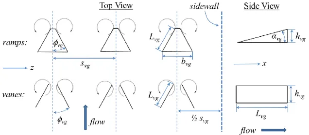
For this work, we have chosen to incorporate the vane-type VGs with rectangular planforms and ramp-type VGs with a triangular wedge shape. Figure 7 shows top and side views of these vortex generators along with the geometric factors defining the VGs. The thick blue arrows indicate the direction of the airflow.
Figure 7. Ramp and vane vortex generators and their vortices.
The key geometric factors of the ramps and vanes are their height (hvg), length (Lvg), and characteristic angle (vg).
The height is expressed with respect to the height of the local boundary layer (hvg/). Traditional vane-type VGs with airfoil shapes tended to have heights comparable to the boundary-layer height [13]. They entrain higher-momentum flow from outside the boundary layer and create vortices that persist well downstream. Micro-scale VGs have heights less than and equal to half of the boundary-layer height. The vortices are created within the boundary layer and quickly dissipate. Because of their smaller size and their presence in the lower-speed flow, the micro-scale VGs have less drag than traditional VGs. The length can be scaled by the height of the VGs in terms of the aspect
ratio of the device (ARvg = hvg/Lvg). For a ramp, the characteristic angle (vg) is the included (apex) angle of the
triangular planform. For a vane, the characteristic angle is the angle-of-incidence of the vane to the local flow. The span of the leading edge of the ramp (bvg) can be determined from the included angle and length of the ramp. The angle of centerline incidence (αvg) of the ramp can be determined from the length and height of the ramp.
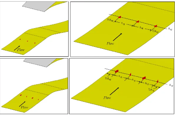
The next set of geometric factors for the VGs are concerned with the placement of the devices onto the inlet surfaces. The key geometric factors are the axial location of the devices (xvg) and the spacing between (svg) devices. The spacing is represented in terms of the height of the device (svg/hvg). A configuration of VGs is a grouping of a number of devices (Nvg) at an axial location (xvg), such as distribution of VGs about the span of the two-dimensional inlet. The number of devices (Nvg) can be determined based on the width of the span of the inlet and the spacing of the devices (svg). Figure 8 shows the placement of the ramps and vanes on the forward ramp of the two-dimensional inlet. The devices are spaced evenly across the span of the inlet. The spacing of ½svg of the VGs from the inviscid sidewalls recognizes that the vortices are essentially reflected about the sidewalls.
The above geometric factorization of the VGs results in the following five geometric factors: height (hvg/), length or aspect ratio (hvg/Lvg), characteristic angle (vg), axial placement (xvg), and spacing (svg/hvg). There exists numerous
possible combinations of factor values. We used guidance from previous investigations in determining a reasonable range of the values of the factors to explore in this work. Anderson et al. [14] applied a design of experiments (DOE) approach to explore the factors for vane and ramp-type VGs for a Mach 2.0 flowfield with an oblique shock/boundary layer interaction. An optimal vortex generator configuration was obtained with a height of hvg/ = 0.4, an aspect ratio of hvg/Lvg = 1.0/7.2 = 0.139, a lateral spacing ratio of svg/hvg = 7.5, and a range of acceptable characteristic angles of
vg = 16 degrees to vg = 24 degrees. These values applied for both the vane and ramp-type VGs.
Hirt et al. [16] experimentally tested the low-boom supersonic inlet (LBSI) in a supersonic wind tunnel, and Rybalko [17] computationally investigated the performance of the LBSI, where both studies maintained cruise speeds at Mach 1.4, similar to the STEX inlet. The upstream devices did not have a significant effect on the boundary layer of the AIP, but were acknowledged for the local flow effects. In contrast, the downstream vane-type VGs substantially reduced the baseline’s radial distortion by 20% to 24%, where the factors were set to hvg/ =0.83 and svg/hvg = 1.0 [17]. The studies cited above did not show improvement in overall AIP pressure recovery or radial distortion when applying guidelines proposed by Anderson [14] for ramp and vane devices.
For the present study of VGs in the two-dimensional inlet, vortex generator heights ranged from the traditional vane-type VGs heights comparable to the boundary layer thickness (hvg/ = 1.0) to micro-scale VGs down to a quarter
Figure 8. Placement of ramps (top) and vanes (bottom) on the forward ramp of the two-dimensional inlet.
of the boundary-layer thickness (hvg/ = 0.25). The aspect ratios of the vanes ranged from hvg/Lvg = 0.25 to 0.50. All vanes had a characteristic angles of vg = ± 16 degrees and all ramps had angles of vg = 24 degrees. The spacing of
the VGs ranged from svg/hvg = 3.0 to 7.0. The study considered axial placements of the VGs on the forward ramp on the external supersonic diffuser ahead of the terminal shock and on the aft ramp within the throat section downstream of the terminal shock. The x-coordinates of the start and end of the forward ramp were x = -0.142 to 0.256 feet, respectively. The axial positions of the VGs on the forward ramp varied from -0.793 xvg -0.093 feet. The x-coordinates of the start and end of the aft ramp were x = 1.056 to 1.802 feet, respectively. The axial positions of the VGs on the aft ramp varied from 1.243 xvg 1.616 feet.
SUPIN was used to rapidly generate grids about the VGs implemented onto the two-dimensional inlet. The VGs were either incorporated onto the flat ramp of the external supersonic diffuser, as shown in Fig. 8, or the aft ramp of the throat section. The simpler flat-plate geometry of the forward and aft ramps allowed easier geometry modeling and grid generation as the geometric factors of the VGs were varied as part of this study. Multi-block, abutting, structured grids were used about the VGs, and the cells were clustered towards the wall to resolve the boundary layers and to capture flow features associated with VGs. Along the VGs, the grid spacing was kept below 5% of the length or height. Thus, smaller VGs resulted in smaller grid spacing about the VGs. The grid spacing about the VGs was gradually increased in the downstream direction to improve resolution the vortices as they propagated downstream to the AIP. Multiple grid blocks were formed to continue this grid refinement between the VGs and the AIP. Thus, the number of grid points for a simulation varied depending on the placement of the VGs and their size. Placement of the VGs on the forward ramp and the smaller size of the VGs resulted in the most grid points. The inlet grid was generated using grid spacing specifications consistent with grid 1 of Table 1; however, the grids about the VGs had much finer grid refinement than grid 3 of Table 1. Grid 1 contained 1.6 million grid points while grid 3 contained 12.8 million grid points. The total number of grid points in the simulations with the VGs varied from about 5 to 25 million grid points.
An alternative to generating grids about each vane-type VG was to use the BAY vortex generator model [18] within the Wind-US code [7]. The BAY model does not require the geometry of the vane to be physically modeled. Rather, the BAY model generates the vortex that the vane could create. The inputs to the model include the grid range that would contain the vane, the angle-of-incidence of the vane, and the planform area of the vane. The BAY model imposes a lifting-force source term within the flow equation and aligns the local flow velocity with the vane incidence.
VI. Results
This section summarizes the results of numerous CFD simulations involving various configurations of the vortex generators. The variation in the inlet performance is summarized and the best-performing vortex generator configurations are discussed. Also discussed are the differences between the gridding of the vortex generators and modeling the vortices using the BAY model.
A. Variation of Inlet Performance
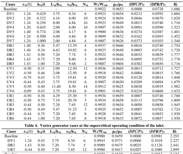
A series of CFD simulations were performed over a range of vortex generator heights, aspect ratios, spacings, and axial placements. Table 3 lists the values of the geometric factors of the VGs and inlet performance metrics for several cases of vortex generator configurations simulated at the critical inlet operating condition. The performance metrics for the baseline inlet with no vortex generators simulated on grid 3 of Table 1 is also listed. The cases with vortex generators are grouped by general location and type as downstream vane (DV), downstream ramp (DR), upstream vane (UV), and upstream ramp (UR). Table 4 lists the values of the factors and inlet performance for select cases simulated at the supercritical inlet operating condition. The cases listed in Tables 3 and 4 are a subset of the total number of cases studied and were chosen to represent the range of factors and the resulting inlet performance at the critical and supercritical operating conditions, respectively.
Figure 9 shows plots of the total pressure recoveries (pt2/pt0) and distortion intensities for the vortex generator cases listed in Tables 3 and 4. The plot of the total pressure recoveries shows the characteristic curve for the baseline inlet. The total pressure recoveries of the cases with VGs at the critical operating condition varied between pt2/pt0 = 0.9602 and 0.9666. An improvement of pt2/pt0 = 0.9666 compared to the baseline inlet value pt2/pt0= 0.9653 is encouraging; however, the variation of the total pressure recovery with grid refinement as listed in Table 1 indicated a variation of pt2/pt0 = 0.0014 between grids 1 and 3. Thus, one has to be cautious of claiming improvement. The plot of total pressure distortion intensities show that the radial distortion descriptor, (DPR/P)2, was able to be reduced down to levels of (DPR/P)2 = 0.0103, which if very encouraging. Generally, it is only sufficient to keep distortion intensities below the limits rather than minimizing the distortion intensities. A lower value at the inlet design condition
provides margin for a possible increase in distortion intensities at off-design conditions. The variation of the incompressible shape factor indicated values as low as Hi = 1.34, which was about a 21% reduction from the baseline value and approached values for a fully turbulent boundary layer on a flat plate.
Table 3. Vortex generator cases at the critical operating condition of the inlet.
Cases xvg(ft) hvg/δ Lvg/hvg svg/hvg Nvg W2/Wcap pt2/pt0 (DPC/P)2 (DPR/P)2 Hi Baseline - - - 0.9922 0.9653 0.0000 0.0728 1.686 DV1 1.24 0.429 3.75 8.34 6 0.9923 0.9654 0.0212 0.0592 1.604 DV2 1.20 0.322 4.16 6.00 10 0.9924 0.9654 0.0046 0.0670 1.620 DV3 1.24 0.250 8.00 4.84 16 0.9923 0.9649 0.0013 0.0740 1.716 DV4 1.20 0.645 2.00 6.00 10 0.9907 0.9639 0.0091 0.0590 1.523 DV5 1.40 0.774 2.08 4.17 6 0.9900 0.9636 0.0274 0.0387 1.401 DV6 1.24 0.500 4.00 4.84 8 0.9899 0.9632 0.0162 0.0493 1.452 DV7 1.24 1.000 2.00 4.84 4 0.9887 0.9626 0.0373 0.0103 1.340 DR1 1.40 0.36 5.47 13.39 4 0.9937 0.9666 0.0016 0.0740 1.754 DR2 1.40 0.34 6.63 10.82 6 0.9923 0.9649 0.0003 0.0742 1.720 DR3 1.43 0.50 7.20 7.74 5 0.9922 0.9644 0.0032 0.0829 1.777 DR4 1.43 0.75 7.20 8.60 3 0.9895 0.9616 0.0095 0.0752 1.778 DR5 1.43 1.00 7.20 9.68 2 0.9887 0.9604 0.0302 0.0656 1.716 UV1 -0.50 0.31 2.00 12.50 12 0.9936 0.9665 0.0013 0.0712 1.727 UV2 -0.50 0.46 2.08 12.50 8 0.9918 0.9642 0.0004 0.0815 1.766 UV3 -0.79 0.43 3.75 19.81 6 0.9920 0.9636 0.0120 0.0814 1.848 UV4 -0.44 0.43 3.75 19.81 6 0.9907 0.9630 0.0209 0.0694 1.679 UV5 -0.50 0.40 11.60 8.30 14 0.9912 0.9625 0.0038 0.0935 1.982 UV6 -0.09 0.43 3.75 19.81 6 0.9901 0.9623 0.0218 0.0660 1.633 UR1 -0.50 0.36 4.29 25.30 5 0.9934 0.9659 0.0007 0.0748 1.760 UR2 -0.50 0.75 7.19 20.39 3 0.9934 0.9658 0.0113 0.0796 1.809 UR3 -0.44 0.50 7.20 7.65 12 0.9935 0.9654 0.0050 0.0858 1.945 UR4 -0.50 0.49 5.47 31.25 3 0.9925 0.9652 0.0007 0.0762 1.724 UR5 -0.44 0.75 7.20 7.65 8 0.9928 0.9647 0.0041 0.0852 1.930 UR6 -0.44 1.00 7.20 7.65 6 0.9918 0.9633 0.0072 0.0857 1.930
Table 4. Vortex generator cases at the supercritical operating condition of the inlet. Cases xvg(ft) hvg/δ Lvg/hvg svg/hvg Nvg W2/Wcap pt2/pt0 (DPC/P)2 (DPR/P)2 Hi Baseline - - - 0.9980 0.9459 0.0000 0.0981 2.293 DV1 1.24 0.43 3.75 8.34 6 0.9943 0.9371 0.0006 0.1018 2.227 DR3 1.43 0.50 7.20 7.74 5 0.9989 0.9475 0.0025 0.1126 2.441 UR3 -0.44 0.50 7.20 7.65 12 0.9980 0.9417 0.0207 0.1089 2.899 Baseline - - - 0.9972 0.9532 0.0000 0.0853 2.123 UV1 -0.50 0.31 2.00 12.50 12 0.9940 0.9495 0.0320 0.0787 2.314
B. Best-Performing Vortex Generator Cases
The following paragraphs examine how effective the type of VGs and their factors were at increasing total pressure recovery, reducing total pressure distortion, and improving the boundary layer. The discussion considers first how the inlet performance metrics varied with the geometric factors for each type of vortex generator and its placement either upstream or downstream of the terminal shock. The “best” case of each grouping is identified. The term “best” is used informally since a formal optimization was not performed. The “best” case is more of a representative case. The discussion then considers the effectiveness with respect to vortex generator type and placement.
The downstream vane (DV) cases of Table 3 did not show real improvement in total pressure recovery relative to the baseline; however, the radial distortion was able to be reduced to (DPR/P)2 = 0.0103 and the incompressible shape factor reduced to Hi = 1.34. Of the four geometric factors varied, the height seemed to have the most impact. As the height increased, the radial distortion and incompressible shape factor improved as indicated by decreased values. The total pressure recovery decreased with increased height, which was likely due to increased drag of the larger VGs. The axial position, aspect ratio, and spacing did not seem to have noticeable effects. Case DV1 was chosen as the “best” case of the downstream vane cases.
The downstream ramp (DR) cases did not seem to really improve any of the inlet performance metrics. Case DR1 indicated a total pressure recovery of pt2/pt0 = 0.9666; however, a very similar case DR2, indicated a recovery of pt2/pt0
= 0.9649. Thus, the value for DR1 was questionable and warrants further investigation. Only case DR5 showed a decrease in radial distortion, which is consistent with a reduction of radial distortion with increased height. Given that none of the downstream ramp cases showed real improvement of the inlet performance metrics, case DR3 was chosen as the “best” case of the downstream ramp cases.
The upstream vane (UV) cases mostly showed a decrease in the inlet performance metrics. Case UV1 did indicate a total pressure recovery of pt2/pt0 = 0.9665 with essentially no improvement in the radial distortion or incompressible shape factor. The height of the vane of case UV1 was hvg/ = 0.31, which was equivalent to the height of the sonic line of the boundary layer. The other upstream vane cases had greater heights and lower total pressure recovery. This suggests that extending the height into the supersonic stream results in greater total pressure loss due to possibly wave drag about the vane. A good practice may be to limit the height of vortex generators on the external supersonic diffuser to below the sonic line of the boundary layer. Case UV1 was chosen as the “best” case of the upstream vane cases.
The upstream ramp (UR) cases did not show any real improvement of the inlet performance metrics. Case UR3 was chosen as the “best” case of the upstream ramp cases.
The “best” cases of Table 3 for the critical operating condition were simulated at supercritical operating conditions. Cases DV1, DR3, and UR3 were simulated at the supercritical point represented by the most-supercritical point of the characteristic curve of Fig. 9 and can be compared to the supercritical simulation of the baseline inlet with grid 3 of
Figure 9. Plots of the total pressure recoveries (left) and distortion intensities (right) for the vortex generator configurations at the critical and supercritical inlet operating conditions.
Table 2. Case UV1 was simulated at the supercritical conditions represented by the second-to-most-supercritical point of the characteristic curve of Fig. 9. Table 4 lists the inlet performance metrics for the supercritical operating conditions. The top-most row labeled “Baseline” provides the inlet performance metrics for the baseline inlet at the most-supercritical point and can be compared to the inlet performance metrics of the supercritical cases of DV1, DR3, and UR3. The lower row labeled “Baseline” provides the inlet performance metrics for the baseline inlet at the next-to-most-supercritical point and can be compared to the inlet performance metrics of the supercritical case of UV1.
Figures 1013 show the Mach number contours for the flow through these “best” cases at the critical and supercritical operating conditions. The vortex generators are colored in red. The vortices from the vortex generators are visible in some of the images as ripples in the Mach number contours. The supercritical simulations show larger low-momentum regions on the centerbody and result in decreased total pressure recovery and increased radial distortion and incompressible shape factor. The supercritical simulations of UV1 and UR3 show an asymmetry of the Mach number contours at the engine face in Figs. 12 and 13, respectively. This suggest possible numerical errors in the simulation that could introduce uncertainty in the values of the inlet performance metrics listed in Table 4.
For the supercritical simulations, the downstream ramp case DR3 did show an increase in the total pressure recovery, but did not improve radial distortion or the incompressible shape factor. The downstream vane case DV1 was not effective. The height of the vane may have been too small to penetrate much into the thicker boundary layer of the supercritical flowfield and provide much mixing of the flow. The upstream vane case UV1 did not seem to be effective at improving the inlet performance at the supercritical operating condition.
Figure 10. Mach number contours of case DV1 at critical (left) and supercritical (right) operating conditions.
Figure 12. Mach number contours of case UV1 at critical (left) and supercritical (right) operating conditions.
Figure 13. Mach number contours of case UR3 at critical (left) and supercritical (right) operating conditions. For the upstream and downstream rotating vane pairs at the critical operating condition, a pair of counter-rotating vortices are produced as the flows reach the trailing edge of the devices. The pressure side of the vane pair is facing towards each other, producing an upwash vortex pair. The suction side of the vane pair is facing away from each other, producing a downwash vortex pair. As the two vortices from the counter-rotating pair move closer to each other, the vortex core area grows further downstream, which is seen later on. The counter-rotating vortices result in significant reduction of low-momentum flow in the separated region of the engine face. The upwash and downwash regions are strongest at the engine face of the subsonic diffuser for downstream vanes compared to upstream vanes at the critical operating condition. On the other hand, the supercritical operating conditions of the counter-rotating vane cases do not represent such vortex growth downstream of the devices.
In Fig. 14, contours of axial velocity normalized by freestream axial velocity (u0) are shown at the AIP. The setup of the counter-rotating devices allows the visualization of primary spanwise vortices and mutually-induced upward velocity. This mutually-induced upward velocity lifts the vortex core and forces the system of vortices to move upward, creating an upwash region followed by a downwash region. The formation of the secondary vortex by viscous effects creates a situation where primary and secondary vortices mutually induce a velocity upon each other. Primary counter-rotating vortex pairs entrain high-momentum fluid in the near-wall region, energizing the boundary layer.
In the top row, the upstream and downstream devices produce a counter-rotating pair of vortices, moving closer together and upward from the wall as it progresses downstream through the inlet. In the middle row, the vorticity contours demonstrate that the vortex pairs are not fully dissipated when they reach the engine face, resulting in some non-zero vorticity. In the bottom row, the axial normalized velocity contours on the plane perpendicular to the flow
direction are subtracted by the baseline axial velocity distribution to easily identify regions of low and high momentum. Blue regions identify reduced flow regions and red regions identify enhanced flow regions.
Baseline UV1 DV1 UR3 DR3
Figure 14. Contours of axial velocity (u/u0, top), vorticity (x, middle) and velocity difference (udiff/u0, bottom) across the span of the AIP.
Taller devices yield more reduced flow and enhanced flow regions than smaller devices. The streamwise vortices will also be more dominant compared to smaller devices, which results in drag of the inlet. Although taller devices may significantly improve the health of the boundary layer, the high momentum flow introduced to the engine face results in non-uniformity, which is undesirable for optimum inlet performance. Implementing smaller devices is critical to preventing complications such as non-uniform flow at the engine face. The smaller devices would allow acceptable inlet performance over the entire flight envelope. The streamwise vortices are weaker compared to the taller devices. This keeps the amount of reduced flow and enhanced flow at a minimum, which does not incur major penalties at the engine face.
In Fig. 15, the case UV1 is depicted at several axial stations, measured from the vane trailing edge and nondimensionalized by the vane height. The vortex dissipates until the point of the normal shock wave boundary layer interaction (NSBLI) at x/hvg 0.60, and then instantaneously increases in magnitude due to the adverse pressure gradients caused by the interaction. This RANS simulation resolves all the features at each axial station for design purposes, including the vortex circulation and decay. Although the vortex is bent due the shock, the vortices still maintain strength as they move downstream in the subsonic diffuser.
Figure 15. Velocity contours of upstream vane case UV1.
C. Gridding of the Vortex Generators Compared to Using the BAY model
As discussed in Section V, an alternative to generating grids about each vane-type vortex generator was to use the BAY vortex generator model within the Wind-US code. In this subsection we compare the use of the BAY model to the approach of gridding about each vane. The case selected for this comparison was equivalent to case DV1 with six vanes placed downstream of the terminal shock; however, the axial placement of the vanes was at xvg = 1.43 feet. Table 5 summarizes the simulations discussed in this sub-section. The “Baseline” simulation is the inlet with no vortex generators at the critical operating condition and is the same as the “Baseline” simulation of Table 3. The “Gridded” simulation is the inlet with the vane configuration discussed in the previous paragraph with each vane gridded. Four CFD simulations were performed using the BAY model. The first simulation with the BAY model is referred to the “Gridded BAY” simulation and used the same grid as the “Gridded” simulation; however, the BAY model was applied rather than using viscous boundary conditions on the vanes. The second through fourth simulations using the BAY model used the three grids of the grid resolution study shown in Table 1. The grids of the “Baseline” and “Grid 3 BAY” simulations are identical. Grids 1 and 2 are coarser grids as discussed in Section IV. The column labeled “Ni-vg” indicates the number of streamwise grid points used to resolve each vane. The column labeled “Ni-sub” indicates the number of streamwise grid points between the end of the vanes and the engine face. This value suggests the level of streamwise resolution of the vortices. The column labeled “Nk-sub” indicates the number of cross-stream grid points used within the span of the inlet and suggests the level of cross-stream resolution used to resolve the vortices. The last five columns of Table 5 list the inlet performance obtained from each of the simulations.
Since vorticity is defined as the difference between velocity gradients, a finely resolved grid of the inlet is desirable for modeling the vortices via the BAY model. The spacing of the grid of the Gridded Bay simulation was equivalent to the gridded vane solution. The equivalence of spacing led to an almost equivalent peak vorticity and axial decay of the gridded vanes. The BAY model was used with Grids 1, 2, and 3, which had coarser grid resolution about the vanes. However, Fig. 16 shows that the peak vorticity was not captured. This was likely due to the coarser grid resolution near the vane.
Table 5. Comparison of gridded vanes with use of BAY model.
Simulations Ni-vg Ni-sub Nk-sub W2/Wcap pt2/pt0 (DPC/P)2 (DPR/P)2 Hi
Baseline - 152 73 0.9922 0.9653 0.0000 0.0728 1.686 Gridded 15 71 549 0.9924 0.9653 0.0173 0.0657 1.660 Gridded BAY 15 71 549 0.9923 0.9653 0.0239 0.0539 1.637 Grid 1 BAY 3 54 27 0.9905 0.9634 0.0239 0.0539 1.540 Grid 2 BAY 5 109 53 0.9901 0.9639 0.0295 0.0437 1.453 Grid 3 BAY 7 152 73 0.9901 0.9643 0.0321 0.0401 1.436 0 100000 200000 300000 400000 500000 600000 700000 800000 0 25 50 75 100 125
Peak
V
or
ti
ci
ty
Δx/h
Gridded Gridded BAY Grid 1 BAY Grid 2 BAY Grid 3 BAYIn Figure 16, the percentage difference between the BAY model and the “Gridded” solution of the downstream vanes are approximately 6%. The gridded model demonstrates a peak vorticity of 650,000 1/s at the first station, and the BAY model demonstrates a peak vorticity of 690,000 1/s. The BAY model slightly overestimated the initial peak vorticity, indicating a slightly larger concentrated vortex compared to the gridded vanes. This is also observed in the decay of the vorticity contours seen in Figure 17. Both cases maintain the same circulation decay downstream of the vanes. Spacing of the BAY model solution was equivalent to the gridded vane solution to maintain high accuracy. Refining the spacing as such lead to almost an equivalent peak vorticity and axial decay of the gridded vanes.
VII. Conclusions
The current study shows that select vortex generator configurations upstream and downstream of the terminal shock/boundary layer interaction can be used to improve the flow at the engine face. Previous studies showed negligible improvement in reducing flow distortion at the engine face when applying proposed design guidelines for ramp and vane devices to the external supersonic diffuser, most likely due to the ARP 1420 regulations for not capturing the near-wall effects. The design guidelines of passive flow control devices proposed by previous studies were modified in order to observe improvement on the external supersonic diffuser or the subsonic diffuser.
Among the cases examined, the improvement in total pressure recovery, radial distortion and incompressible shape factor were found in 6, 8, and 17 cases, respectively. The trends indicated that higher total pressure occurs at lower
h/δ values. The increasing total pressure recovery is observed for (1) DV cases at constant s/h and 𝑥𝑣𝑔 at decreasing
h/δ, (2) DR cases at constant L/h and 𝑥𝑣𝑔at decreasing h/δ, (3) UV cases at constant h/δ, L/h and s/h at decreasing 𝑥𝑣𝑔, and (4) UR cases at constant 𝑥𝑣𝑔, L/h and s/h at decreasing h/δ.
The study indicates that the smaller devices perform better than the larger devices at improving the flow at the engine face. This is due to the weaker vortex filaments of the smaller devices sufficiently dissipating before the engine face while the larger devices produce large amounts of reduced and enhanced flow at the AIP that could persist past the engine face. The larger devices that result in total pressure recovery losses due to increased height also result in increased drag, which is detrimental for inlet performance.
The best performing devices in terms of reducing radial distortion and improving the boundary layer are downstream vanes. Reduction in radial distortion improves the operability of the inlet and may as well reduce the unsteadiness in the normal shock wave motion. The downstream vanes were second to upstream vanes in terms of reducing radial distortion. Both upstream and downstream ramps were not as effective in reducing radial distortion as the latter. In the study, the device height was the most effective parameter compared to device axial placement, spacing and length. As previously discussed, the STEX inlet varies the low-momentum boundary layer circumferentially due to a streamline-traced method, which introduces complexity compared to the two-dimensional inlet. The two-dimensional inlet has a constant low-momentum region and planar flow at the engine face. Due to the complexity of the STEX inlet, a formal DOE approach will be applied in the future to statistically determine the interaction between all the VG factors.
Acknowledgements
The first author gratefully acknowledges support from the NASA Harriett G. Jenkins Graduate Fellowship Program. The authors also acknowledge the access to NASA’s computing resources. The work was supported in part by the Commercial Supersonic Technology Project of the NASA Advanced Air Vehicles Program.
References
[1] Goldsmith, E.L. and Seddon, J., Practical Intake Aerodynamic Design, AIAA, Washington, DC, 1993.
[2] Slater, J.W., “Methodology for the Design of Streamline-Traced, External-Compression Inlets,” AIAA Paper 2014–3593, 2014.
[3] Otto, S.E, Trefny, C.J. and Slater, J.W, “Inward-Turning Streamline-Traced Inlet Design Method for Low-Boom, Low-Drag Applications,” AIAA Paper 2015–3593, 2015.
[4] Slater, J.W., “Enhanced Performance of Streamline-Traced External-Compression Supersonic Inlets,” ISABE Paper 2015–22049, 2015.
[5] Slater, J.W., “Design and Analysis Tool for External-Compression Supersonic Inlets,” AIAA Paper 2012–0016, 2012.
[6] Slater, J.W., “SUPIN: A Computational Tool for Supersonic Inlet Design,” AIAA Paper 2016–0532, 2016. [7] Yoder, D.A., ‘Wind-US User’s Guide: Version 3.0,” NASA TM 2016-219078, March 2016.
[8] Menter, F.R., “Zonal Two Equation Kappa-Omega Turbulence Models for Aerodynamic Flows,” AIAA Paper 93-2906, 1993.
[9] Society of Automotive Engineers (SAE), “Gas Turbine Engine Inlet Flow Distortion Guidelines,” SAE ARP 1420, Rev. B, February 2002.
[10]Braun, E.M., Lu, F.K. and Wilson, D.R., “Experimental Research in Aerodynamic Control with Electric and Electromagnetic Fields,” Progress in Aerospace Sciences, Vol. 45, No. 1–3, 2009, pp. 30–49.
[11]Fukuda, M.K., Hingst, W.G., and Reshotko, E., “Bleed Effects on Shock / Boundary-Layer Interactions in Supersonic Mixed Compression Inlets,” AIAA Journal of Aircraft, Vol. 14, No. 2, February 1977, pp. 151-156. doi: 10.2514/3.58756.
[12] Lu, F. K., Pierce, A. J., Shih, Y., Liu, C., and Li, Q., “Experimental and Numerical Study of Flow Topology Past Micro-Vortex Generators,” AIAA Paper 2008–4463, 2010.
[13]Cubbison, R.W., Meleason, E.T., and Johnson, D.F., “Performance Characteristics from Mach 2.58 to 1.98 of an Axisymmetric Mixed-Compression Inlet System with 60-Percent Internal Contraction,” NASA-TM-X-1739, February 1969.
[14]Anderson, B.H., Tinapple, J. and Surber, L., “Optimal Control of Shock Wave Turbulent Boundary Layer Interactions Using Micro-Array Actuation,” AIAA Paper 2006–3197, 2006.
[15]Lee, S., Loth, E. and Babinsky, H., “Normal Shock Boundary Layer Interaction Control Using Micro-Vortex Generators,” AIAA Paper 2010–4254, 2010.
[16]Hirt, S.M., Chima, R.V., Vyas, M.A., Wayman, T.R., Connors, T.R. and Reger, R.W., “Experimental Investigation of a Large-Scale Low- Boom Inlet Concept,” AIAA Paper 2011–3796, 2011.
[17]Rybalko, M., and Loth, E., “Aerodynamic Impact of Vortex Generators on a Relaxed-Compression Low-Boom Inlet,” AIAA Journal, Vol. 53, No. 12, pp. 3700–3711. doi: 10.2514/1.J054050
[18]Dudek, J.C., “Modeling Vortex Generators in a Navier-Stokes Code”, AIAA Journal, Vol. 49, No. 4, April 2011, pp. 748-759. doi: 10.2514/1.J050683.
[19]Lu, F.K., Li, Q., and Liu, C., “Microvortex Generators in High-Speed Flow,” Progress in Aerospace Sciences, Vol. 53, 2012, pp. 30–45. doi: 10.1016/j.paerosci.2012.03.003