Laser-Control of Molecular Dynamics. Dissertation

(1)

Laser-Control of Molecular

Dynamics

Dissertation

zur Erlangung des

naturwissenschaftlichen Doktorgrades

der Bayerischen Julius-Maximilians-Universit¨at W¨urzburg

vorgelegt von

Stefanie Gr¨

afe

aus

D¨usseldorf

(2)

(3)

Eingereicht am: . . . . bei der Fakult¨at f¨ur Chemie und Pharmazie

1. Gutachter: . . . . 2. Gutachter: . . . . der Dissertation 1. Prüfer: . . . . 2. Prüfer: . . . . 3. Prüfer: . . . . des Öffentlichen Promotionskolloquiums

Tag des ¨Offentlichen Promotionskolloquiums: . . . .

(4)

(5)

Introduction

With increasing knowledge about the structure and dynamics of molecules, the goal to not only observe, but to actively control chemical processes has been approached in the last decades. The development of pulse shapers [1] makes it possible to phase- and amplitude-modulate electromagnetic fields to be employed to influence atoms, molecules and solid state systems in a desired way. Theoreti-cal, as well as experimental efforts along these directions are summarized in two recent monographs [2, 3] and numerous review articles [4–8].

Several activities originated from research groups in W¨urzburg (supported within the Sonderforschungsbereich 347) where organometallics like Fe(CO)5 [9],

and also organic polymers [10, 11] were selectively dissociated or excited, respec-tively. A generic control scheme is visualized in fig. 1.

Figure 1: General scheme for a controlled dissociation of a molecule A – B – C. After an excitation process one bond, either the A – B or the B – C bond, is broken selectively.

(10)

2 INTRODUCTION

For a molecule A – B – C with two different bonds, the objective of control is to selectively excite or break one of these bonds. Various control theories have been developed to achieve this “selective bond-breaking”. The intuitive Tannor–Rice– Kosloff scheme employs the explicit time-dependence of wave packets prepared by ultrashort laser pulses [12, 13]. Starting from an initial state ψ0, a first pulse

excites the molecule. The branching ratio between competing reaction channels of the system can be controlled by timing a second laser pulse correctly. Figure 2 illustrates the excitation scheme. After the excitation, dynamical processes take place in the excited state (ψ∗₍_t_{)). Depending on the system’s properties, a}

second laser excitation taking place at different times T1, T2 is able to produce

alternatively products of type (1) or (2).

Figure 2: Tannor – Rice – Kosloff scheme: After a first excitation, a second laser pulse fired at different times populates one or the other reaction channel.

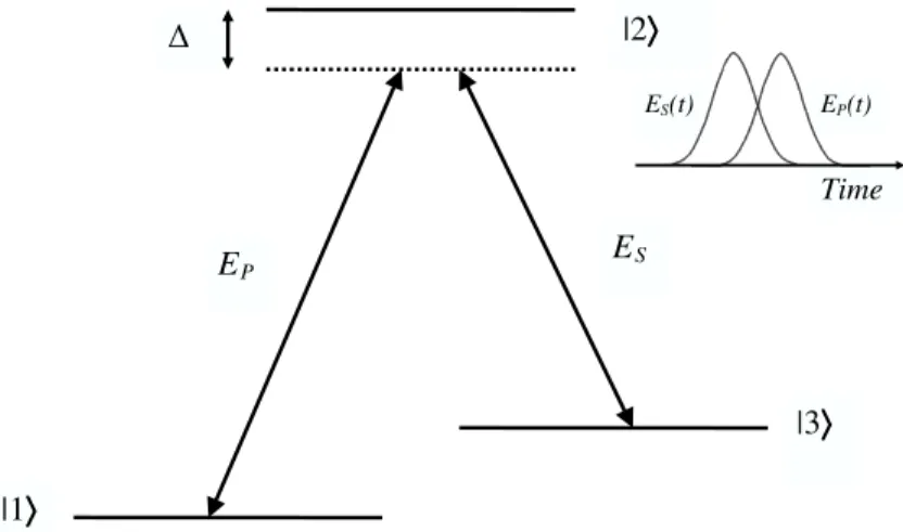
Within the STIRAP (acronym for “stimulated Raman adiabtic passage”) method a population transfer is performed employing time-delayed pulses in a counter-intuitive sequence [14]. Thereby, the population in the excited state _|2_i in the so-called Λ- configuration (see fig. 3) is negligible for all times. In a physi-cal picture, this strong-field phenomenon is explained with a strong perturbation induced by the first pulse, the Stokes pulse, inducing the formation of new

(11)

“field-INTRODUCTION 3

Figure 3: Population transfer for a three-level system in the so-calledΛ-configuration. Two pulses in a counter-intuitive pulse sequence, pump- (E_P(t)) and Stokes-pulseE_S(t)

couple the three levels, as indicated. Within the STIRAP-process the excited state

|2_i which may be not resonantly accessible because of an energy detuning ∆ is not populated remarkably at all times.

dressed” states. The second pulse, the pump-pulse, then transfers population along one of these states, avoiding the excited state _|2_i.

Brumer and Shapiro developed a method to control reaction yields via in-terference effects of phase-varied laser pulses [15, 16]. Competing multiphoton pathways to access a final state are marked with a phase difference which then leads to an interference – very much like in Young’s double-slit experiment.

Variationally derived control fields relying on an overlap of a system’s wave-function with a target state being maximized, are iteratively determined within optimal control theory [17, 18]. Therefore, the system’s initial state is forward propagated while, with the backward propagated target state the time-dependent overlap of the states is used to construct the electric field.

In a combination of pulse-shaping techniques and feedback from a (mea-sured or calculated) signal, control fields can be obtained adapting genetic algo-rithms [19]. Starting from a random distribution, the driving field is determined

(12)

4 INTRODUCTION

by random modification of parameters in terms of the biological evolution in a parallel search.

In most of the above described techniques, the derived control fields are diffi-cult to interpret in terms of the system’s properties. In order to gain insight into the entanglement of the applied perturbation and the molecular dynamics, an algorithm is developed within this work which determines the control fields from the instantaneous response of the system. This extents early work of Tannor and others [20–23].

The principle can be visualized in regarding a classical particle moving along a trajectory in an anharmonic potential. An increase of the particle’s energy as a function of time is achieved if an external field is constructed propotional to the instantaneous momentum of the particle. In contrary, the particle’s energy decreases in choosing the external field to be phase shifted to the momentum. Figure 4 illustrates the case where a heating of a particle moving in a Morse potential occurs. The particle’s energy increases in a Morse potential (panel (a)) and the trajectory (panel (b)), as well as the field, driving the system in resonance is shown (panel (c)).

The such established “principle of instantaneous control” is applied to vari-ous molecular processes in this work [24–26]. Therefore, different objectives are defined as the energy transfer in double well potentials, the excitation and disso-ciation of selective vibrational modes, and also the population transfer between molecular electronic states.

This work is organized as follows: The first three chapters summarize the employed theoretical (chapter 1) and numerical methods (chapter 2), as well as several control theories (chapter 3).

(13)

INTRODUCTION 5

Potential Energy

Coordinate Coordinate Field Intensity

Time

(a) (b) (c)

Figure 4: Panel (a): A classical particle’s trajectory in a Morse potential; panel (b) displays the trajectory depending on time, driven by a control field in panel (c). The dashed lines indicate times where the trajectory is at a classical turning point, and the electric field is zero.

The application of the instantaneous response algorithm to energy transfer problems is presented in chapter 4. Relating the control fields to the vibrational dynamics, it is shown that taylored IR-fields are able to effectively heat or cool molecules.

Selective mode excitation leading to dissociation is studied for the HOD-molecule in chapter 5. Here, control fields are constructed to break one or the other bond within the electronic ground state.

The population transfer via non-resonant excitation into excited electronic states is investigated in chapter 6. Here, the control fields derived from optimal control theory, genetic algorithms and the instantaneous response are compared for a model system representing methyl iodide.

Chapter 7 investigates selective population transfer in the sodium dimer. The structure of the control fields is related to the vibrational and electronic dynamics of the molecule. Orientational as well as field–strength effects are examined and

(14)

6 INTRODUCTION

time–resolved pump/probe spectroscopy is shown to yield information about the efficiency of control processes [27].

In cooperation with experimental investigations on molecular iodine, a STI-RAP-like technique is transferred into the femtosecond–regime. It is shown that field dressed states and an adiabatic description are proper tools in characterizing population transfer into highly excited vibrational eigenstates without populating an excited electronic state remarkably. The motivation is to initiate a ground state dynamics on a time scale much faster than those of decoherence processes.

(15)

Chapter 1

Theory

1.1

Dynamical Equations

The dynamical properties of a system can be described within two different for-malisms, the latter being classical mechanics and quantum mechanics. For macro-scopic systems the methods of classical mechanics are appropiate, while these approaches are likely to fail for atoms and molecules because of their quantum mechanical attributes. In this section the classical and quantum dynamical equa-tions of motion and their soluequa-tions will be reviewed. The equaequa-tions are generally given for vectors if not denoted differently.

1.1.1

Classical Dynamics

Molecular dynamics (MD) methods employ the equations of classical mechanics to determine the properties of a system. Considering a particle with massm and generalized coordinate x, the Lagrangian function _L, defined as the difference between the kinetic T and the potential energy V reads [28, 29]

L= m 2x˙

2₋_V₍_x₎_, _(1.1)

(16)

8 1.1. DYNAMICAL EQUATIONS

where ˙xis the time derivative ofx. The resulting (Lagrangian) equation of motion then is d dt ∂_L ∂x˙ ! − ∂L ∂x = 0. (1.2)

To ease the transition to quantum mechanics, Hamiltons formulation is adopted in defining the momenta p

p= ∂L

∂x˙. (1.3)

The Hamilton function _H, the sum of kinetic and potential energy (_H =T +V), is related to _L via a Legendre transformation:

H=_H(x,x, p˙ ) =px˙ _{− L}(x,x, t˙ ). (1.4) The canonical or Hamilton’s equations of motion read:

∂_H ∂p = ˙x;

∂_H

∂x =−p.˙ (1.5)

The Hamilton function describes the system’s energy. For ˙_H = 0, energy con-servation law applies. In the case of a time-dependent external potential, e.g. a classical laser field acting on the system, the equations of motion are, in general, solved numerically (see chapter 2). For an ensemble of particles a trajectory en-semble _{xi} can be propagated and statistically weighted with a probability Pi to construct a classical density ρ(t). Depicting the classical density, each xi is smoothed by a (Gaussian) distribution around this particular point

ρ(x, t) =X i

e−β(x−xi)2_P

i. (1.6)

The classical density’s motion is expressed by the classical Liouville equation dρ dt = ∂ρ ∂t + " ∂ρ ∂xi ˙ xi+ ∂ρ ∂pi ˙ pi #

(17)

CHAPTER 1. THEORY 9 = ∂ρ ∂t + " ∂ρ ∂xi ∂_H ∂pi − ∂ρ ∂pi ∂_H ∂xi # = 0. (1.7)

As the density ρ does not change along a trajectory, the total time derivative of the density vanishes. Therefore, the equation of motion can be re-written using poisson brackets

∂

∂tρ=− {ρ,H} (1.8)

For a density describable by aδ-function, eq. (1.8) transforms to Newton’s equa-tions of motion [30].

1.1.2

Quantum Dynamics

The Hamiltonian formulation of classical dynamics can be transferred to quan-tum dynamics by some modifications [31]. A similar picture as the classical density can be regarded for a quantum mechanical description if assigning the classical variables to corresponding quantum mechanical operators (principle of correspondence). Operators representing physical observables have to be Her-mitian. The vectors xi(t) are assigned to the complex linear vectors _|ψ(x, t)i_i describing a state in Hilbert space (Born’s proposal) [32]. The corresponding equation of motion for the state vectors describing a quantum mechanical system is the time-dependent Schr¨odinger equation

i¯h∂

∂t|ψ(t)i= (T +V) |ψ(t)i=H |ψ(t)i, (1.9) where _H is the quantum mechanical Hamiltonian. Its precise form (within the Born-Oppenheimer approximation) will be described in the next subsection, since for molecules in a quantum mechanical picture, as treated here, it is in general difficult to examine the dynamics of nuclei and electrons simultaneously.

(18)

10 1.1. DYNAMICAL EQUATIONS

In order to describe a quantity in analogy to the classical picture, a density operator ρ is defined

ρ(t)_{≡ |}ψ(t)_ihψ(t)_|. (1.10) Therefore, the quantum mechanical analogon of the classical density, the density matrix, can be written as

ρ(x, t) =X i

Pihx|ψi(t)i hψi(t)|xi, (1.11) with the probability distribution Pi. Integration over a volume V yields

Z V ∂ ∂tρ dx= d dt Z V ρ dx= 0, (1.12)

where the divergence theorem was used. Eq. (1.12) describes the global con-servation property, meaning that the integral of _|ψ_|2 _{is independent of time - or}

rescaling for V _→R3 _{(Hilbert space)}

Z

R3|ψ|

2_dx_{= 1}_. _(1.13)

The corresponding equation of motion (Liouville – Von Neumann equation) for the density matrix is

∂

∂tρ=− i ¯

h [H, ρ]. (1.14)

Thereby, i/¯h times the commutator is used in analogy to the poisson brackets of classical mechanics. In the case of a pure state (Pi =δi1 in eq. (1.11), |ψ1i) the

system is uniquely described (within non-relativistic quantum mechanics) by the time-dependent Schr¨odinger equation. The solutions of eq. (1.9) can be repre-sented in the complete and orthonormal basis set consisting of eigenvectors _|φni

(19)

CHAPTER 1. THEORY 11

of _H having energies En defined by the time-independent Schr¨odinger equation

H|φni=En|φni. (1.15)

Thus one obtains:

|ψ(t)_i=X

n |

φnihφn|ψ(t)i. (1.16)

The time evolution can be expressed by a time evolution operatorU(t, t0)

U(t, t0) =

X

n |

φnie−i/¯hEn(t−t0)hφn|. (1.17) Expanding an arbitrary function f(_H) into a Taylor series one obtains

f(_H) = ∞ X i=0 f(i)₍₀₎ i! H i f(_H)_|φji = ∞ X i=0 fi₍₀₎ i! H i j|φji ≡f(Ej)|φji ⇒U(t, t0) = e−i/h¯H(t−t0). (1.18)

The above specified propagator is only valid for time-independent Hamiltoni-ans. Including a classical external radiation field the Hamiltonian becomes time-dependent and the propagator is of a different form. Employing a classical ap-proximation (see next section) for the field-matter coupling term W(t) yields

H(t) =_H0+W(t). (1.19)

A differential equation for the propagator can be derived when inserting the time evolution _|ψ(t)_i=U(t, t0)|ψ(t0)i into the time-dependent Schr¨odinger equation

∂

∂tU(t, t0)|ψ(t0)i=− i ¯

(20)

12 1.1. DYNAMICAL EQUATIONS

As this equation is valid for any _|ψ(t0)i the propagator must also satisfy

∂

∂tU(t, t0) =− i ¯

hH(t)U(t, t0). (1.21)

Integrating the differential equation from time t0 to t together with the initial

condition U(t0, t0) = 1 results in the integral equation

U(t, t0) = 1− i ¯ h Z t t0 dτ_H(τ)U(τ, t0) (1.22)

which can be solved iteratively leading to the Dyson-series U(t, t0) = 1 + ∞ X n=1 −i ¯ h nZ t t0 dτn Z τn t0 dτn−1· · · Z τ2 t0 dτ1H(τn)H(τn−1)· · · H(τ1). (1.23) Here the time variables are fully orderedt_≥τn≥ · · · ≥τ1 ≥t0 (for commutating

Hamiltonians the ordering would be of no relevance) and the positive time-ordered exponential can equivalently be denoted as

U(t, t0) = exp+ −i ¯ h Z t t0 dτ_H(τ) . (1.24)

1.1.3

Born-Oppenheimer Approximation

The Hamiltonian describing a molecular system (neglecting spin-orbit interac-tions) is given as [33]

H=Te(x) +Tn(R) +V(x, R), (1.25)

where x, R denote the electronic and nuclear coordinates, respectively. The ki-netic energy operators of electrons Te(x) and nuclei Tn(R), and the potential energy operator V(x, R) for a Coulomb system without external forces can be

(21)

The equations above containme, Mα, the electron’s and nuclei’ masses, the gra-dients _∇i =∂/∂x, ∇α =∂/∂R, and the indices (i, j),(α, β) numbering electrons and nuclei, respectively. Expanding the complete wave function ψ(x, R) into a basis of electronic wave functions ϕi(x, R) yields

ψtot(x, R) =

X i

ϕi(x, R)χi(R), (1.27)

with the expansion coefficients χi(R) representing functions of the nuclear coor-dinates. The electronic wave functions are solutions of the electronic Schr¨odinger equation

He(x, R)ϕi(x, R) =i(R)ϕi(x, R). (1.28) Here, i is the electronic quantum number of the electronic state. The i(R) are the potential curves parameterically depending on the nuclear coordinates, and He(x, R) denotes the electronic Hamiltonian

He(x, R) =Te(x) +V(x, R), (1.29)

so that

(22)

14 1.1. DYNAMICAL EQUATIONS

Inserting the basis set expansion into the Schr¨odinger equation yields X i (Tn+He) ϕi(x, R)χi(R) = Etot X i ϕi(x, R)χi(R). (1.31) As the kinetic energy operator is a differential operator it transforms the coupled equations X i X α −¯h2 2Mα∇ 2 α+He ! ϕiχi = Etot X i ϕiχi X i ( X α −¯h2 2Mα∇ 2 α(ϕiχi) +Heϕiχi ) = Etot X i ϕiχi X i ( X α −¯h2 2Mα∇α [(ϕi∇αχi) + (χi∇αϕi)] +χiHeϕi ) = Etot X i ϕiχi(1.32) X i ( X α −¯h2 2Mα ϕi ∇2 αχi +X α −h¯2 Mα (_∇αϕi) (∇αχi) +X α −¯h2 2Mα χi ∇2αϕi +χiiϕi ) = Etot X i ϕiχi Projection on the basis vector _hϕj| results in the coupled set of equations:

X α −¯h2 2Mα∇ 2 αχj+jχj + X i ( X α −h¯2 Mαh ϕj|∇α|ϕii(∇αχi) +X α −¯h2 2Mαh ϕj ∇2α ϕiiχi ) = Etotχj.(1.33)

In equation (1.33), the electronic wave functions are comprised in the terms inside of the curly brackets, kinetically coupling different electronic states. Within the adiabatic approximation off-diagonal kinetic coupling terms (first and second order non-adiabatic coupling elements) are neglected, leading to a separation of electronic and nuclear degrees of freedom. For the electronic eigenstates being real functions, the diagonal non-adiabatic coupling elements (_hϕj|∇α|ϕji) are

(23)

CHAPTER 1. THEORY 15

likewise zero using the orthonormality condition. Equation (1.33) then reads as X α −h¯2 2Mα∇ 2 α+j+ X α −¯h2 2Mαh ϕj ∇2α ϕji ! χj =Etotχj Tn+j + X α −¯h2 2Mαh ϕj ∇2 α ϕji ! χj =Etotχj, (1.34)

where in the second equation the kinetic energy operator was re-introduced. The matrix elements −¯h2

2Mαhϕj|∇

2

α|ϕji are known as the diagonal correction, being smaller than j because the masses of the nuclei enter into the denominator. In the Born-Oppenheimer approximation [34] these slowly inRvarying functions are neglected and the energy surface is solely determined byj. Thus the Schr¨odinger equation for the nuclear motion in state j reads:

[Tn+j(R)]χj(R) =Etotχj(R), (1.35)

where the electronic energyj represents the potential energy surface in the elec-tronic statej.

1.2

Design of Electro-Magnetic Fields

The exact form of the Hamiltonian in eq. (1.19) can be derived from field quan-tization in quantum electrodynamics. Regarding the field-matter interaction of a particle with massm and charge q in an electromagnetic field given by [35, 36]

E =₋1 c

∂A

(24)

16 1.2. DESIGN OF ELECTRO-MAGNETIC FIELDS

where E is the electric field with vector potential A and scalar potential Φ, and B represents the magnetic field, results in a Hamiltonian

H= 1 2m p₋ q cA(x, t) 2 +qΦ(x, t). (1.37)

The canonical momentum p is replaced by the kinetical momentum operators mx˙ =p₋q/cAwhose commutators satisfy slightly different conditions ([xi, mx˙j] =

ihδ¯ ij, [mx˙i, mx˙j] =i¯hqijkBk). In the limit of large photon numbers the electric

field can be treated classically and described as E(x, t) =E0f(t)

h

eikx−iωt₊_e−ikx+iωti

. (1.38)

with the pulse envelope f(t), andE0 is half of the field strength. The first term in

eq. (1.38) corresponds to light absorption and the second to light emission. Since usually molecules are much smaller than the optical wavelength of an external field, the dipole approximation can be adopted which amounts to a neglection of the position dependency, i.e.:

E(t) =E0f(t)

h

e−iωt₊_e+iωti

. (1.39)

Therefore, the form of the external coupling W(t) introduced in the last section can be denoted as the projection of the electric field vectorE(t) onto the system’s dipole moment µ,

W(x, t) =₋µ E(t). (1.40)

The laser fields used and calculated in this work are often composed of different frequencies (shaped) or are modulated in frequency- or time domain. Electric fields in time E(t) and frequency domain E(ω) are connected by the Fourier

(25)

CHAPTER 1. THEORY 17 relation [37] E(t) = √1 2π Z ∞ −∞ ˜ E(ω)eiωtdω ˜ E(ω) = √1 2π Z ∞ −∞E(t)e −iωt_dt _(1.41)

SinceE(t) is always a real quantity the relation in frequency domain is symmetric ˜

E(₋ω) = ˜E∗₍_ω_{). For a full characterization of the electric field it is sufficient to}

regard positive frequencies. The related (complex) temporal fields can be written for positive and negative ω

E+(t) = √1 2π Z ∞ 0 ˜ E(ω)eiωtdω E−(t) = √1 2π Z 0 −∞E(ω)e −iωt_dω. _(1.42)

Therefore, E−₍_t_{) = [}_E+₍_t_)]∗_{, and} _E₍_t_{) =} _E+₍_t_{) +}_E−₍_t_{) = 2}_<₍_E+₍_t_{)). For}

further calculations it is advantageous to regard the E+₍_ω_{), as only} _ω _≥ _{0 is}

physically meaningful. These fields can be described by an envelope function f(t) (g(ω)) and a phase ϕ(t) (φ(ω)). Mathematically a phase modulation is im-plemented by expanding the time-dependent phaseϕ(t) into a Taylor series:

ϕ(t) =ω(t0) + ∂ϕ(t) ∂t t0 (t₋t0) + 1 2 ∂2_ϕ₍_t₎ ∂t2 t0 (t₋t0)2 +· · ·, (1.43)

where the first term is the constant phase of the field, the second indicates the carrier frequency, and the third one is a linear chirp in time domain. Higher order terms in general are called (n-1) order chirps. Pulses with temporally increasing frequency, exhibiting a positive linear chirp are called up-chirped pulses; the op-posite behaviour is called down-chirped, accordingly. Introducing a time-domain chirp changes the spectral distribution of the pulse, not corresponding to the experimental setup where the spectral width remains constant and chirping is

(26)

18 1.2. DESIGN OF ELECTRO-MAGNETIC FIELDS

performed in frequency domain (e.g. routing the pulse through dispersive media or grating dispersion). Expanding the frequency dependent phase into a Taylor series leads to [38, 39]: φ(ω) = φ(ω0) +α1 ∂φ(ω) ∂ω _ω 0 (ω₋ω0) +α2 ∂2_φ₍_ω₎ ∂ω2 _ω 0 (ω₋ω0)2+· · ·. (1.44)

Analogously, the constant term determines the position in time domain, the sec-ond term indicates a temporal displacement and the third one displays a linear chirp in frequency domain. A linear dependency (i.e. only the first and second term contribute) is again called unchirped in frequency domain. The appearence of pulses in the particular domain after a Fourier transform is not easy to derive. Nevertheless, from symmetry it can be said that a pulse possessing an asymmet-ric distribution in one domain cannot be unchirped in the other. An important case is a Gaussian laser pulse

E+(t) = E0 2 e −2 ln 2·t2_/τ2 ·eiω0t _(1.45) ˜ E+(ω) = E0τ r _π 4 ln 2e −τ2₍_ω₋_ω 0)2/(8 ln 2)_, _(1.46)

where τ is the pulse duration, the width at half maximum of the intensity-envelope function I(t) = 0E(t)2, and ω0 is the carrier frequency. A special

feature of Gaussian pulses is that, applying a linar chirp in frequency domain 1/2φ00₍_ω

0)·(ω−ω0), also implies a linear chirp in time domain. The resulting

fields have the analytical form E+(t) = E0 2γ1/4 e −t2_/₄_βγ ·ei(δt2−) ·eiω0t _(1.47) ˜ E+(ω) = E0τ r π 4 ln 2e −τ2₍_ω₋_ω₀₎2_/_{(8 ln 2)} ·ei(ω−ω0)2φ00/2_, _(1.48)

(27)

CHAPTER 1. THEORY 19 with β= τ 2 8 ln 2, γ = 1 + φ002 4β2, δ = φ00 8β2_γ = 1/2 arctan( φ00 2β). (1.49) The temporal broadening as a result of the linear chirp in frequency domain is expressed in τ2 τ1 = v u u t1 + φ 00_{4 ln 2} τ2 1 !2 . (1.50)

It can be seen that the pulse duration for a chirped pulse (τ2) depends on one

hand on the chirp φ00 _{and on the other, on the pulse duration of the unchirped}

pulse (τ1). The resulting broadening has been calculated for Gaussian pulses

before and can be taken from tables in the literature [38].

1.3

Weak Field Regime: Time-Dependent

Per-turbation Theory

Perturbation theory is appropriate for the description of systems with a weak time-dependent interaction V(t) in the Hamiltonian of eq. (1.19), with being a small dimensionless parameter [31]. For timest < t0, the perturbationV(t) = 0

and the system is in an initial state_|ψ(t0)isatisfying the Schr¨odinger equation

i¯h∂

∂t|ψ(t0)i=H0|ψ(t0)i. (1.51) When the perturbation sets in, a new state _|ψ(t)_i develops fulfilling the new Schr¨odinger equation

i¯h∂

(28)

20 1.3. TIME-DEPENDENT PERTURBATION THEORY

with the initial condition _|ψ(t)_i=_|ψ(t0)i for t ≤t0. The temporal development

of the wave function can be described with the afore defined propagator in eq. (1.18)

|ψ(t)_i=U(t, t0)|ψ(t0)i, (1.53)

whereU(t, t0) satisfies eq. (1.21). ForV(t) is assumed to be a small perturbation,

the propagator U can be expressed differing only by a small amount from the unperturbed propagator U0. One then writes

U =U0W, (1.54)

where W is an unitary operator implicating the interaction effects. Inserting the form of U from eq. (1.54) into the Schr¨odinger equation eq. (1.21) yields

i¯h∂ ∂tW(t, t0) = U † 0(t−t0)V(t)U0(t−t0)W(t, t0). (1.55) Combining U0†(t−t0)V(t)U0(t−t0)≡Vint(t, t0), (1.56)

the solutions of W(t, t0) can be expanded into a series

W(t, t0)∼

∞

X

n=0

nWn(t, t0). (1.57)

Time integration of the resulting recursive set of differential equations forn _≥0: i¯h∂

∂tWn+1(t, t0) =Vint(t, t0)Wn(t, t0), (1.58) and the intial condition W(t0, t0) = 1 yields terms of nth order, each form given

by the previous equation

W1(t, t0) = 1 ih¯ Z t t0 Vint(τ, t0)dτ (1.59)

(29)

CHAPTER 1. THEORY 21 W2(t, t0) = 1 i¯h Z t t0 Vint(τ, t0)W1(τ, t0)dτ ... Wn+1(t, t0) = 1 i¯h Z t t0 Vint(τ, t0)Wn(τ, t0)dτ.

The integral equation results in the Dyson series; its solutions can be obtained via iterative insertion of term n into n+ 1. Later, we will refer to cases where the series can be truncated after the first term, describing first-order transitions.

1.3.1

Fermi’s Golden Rule

The probability amplitude of a transition under the action of a weak external potential V(t) starting from a system in an eigenstate _|i(t0)i, whose temporal

development can be expressed according to eq. (1.17), into a final state_|f(t)_i is given by [31]

Ai→f(t, t0) = hf|U(t, t0)|ii

= e−i/¯hEf(t−t0)_h_f_|_W₍_{t, t}

0)|ii. (1.60)

Because the transition probability is the absolute square of the transition am-plitude and defining the transition frequency ωf i = (Ef −Ei)/h¯, the expression reads as |A(t)_|2 = 2 ¯ h2 Z t t0 eiωf i(τ−t0)_h_f_|_V₍_τ₎_|_i_i_dτ 2 . (1.62)

(30)

22 1.3. TIME-DEPENDENT PERTURBATION THEORY

Considering an absorption process with V(t)_≈µexp (₋iωt) and real eigenstates |i_i,_|f_ithe transition probability can be expressed as

|A(t)_|2 = 2 ¯ h2 " sin[(ω₋ωf i)t/2] (ω₋ωf i)/2 #2 |hf_|µ_|i_i|2. (1.63)

The expression in the squared brackets is related to the δ function via lim

T→∞

sin2αT

α2_T =πδ(α), (1.64)

so for long times the transition probability is given by lim T→∞|Ai→f(T)| 2 ₌_t2π ¯ h δ(¯hω+Ef −Ei)|hf|µ|ii| 2 . (1.65)

Therefore, the transition rate Γif (transition probability per time) can evaluated: Γif _≡ 2π

¯

h δ(¯hω+Ef −Ei)|hf|µ|ii|

2

. (1.66)

For a transition from a discrete initial to a final state in a continuous spectrum the above equation has to be integrated taking into account the density of states %(Ef). The number of eigenstates in the interval dEf is calculated from the density of states for %(Ef)dEf and the transition rate is

X f Γif _∼ Z dEf%(Ef)Γif =%(Ei) 2π ¯ h |hf|µ|ii| 2 . (1.67)

(31)

CHAPTER 1. THEORY 23

1.4

Strong Field: Rabi Oscillations

The strong coupling of a two-level system with the eigenstates_|ϕai,|ϕbi with an external radiation field cannot be described by perturbation theory. The state vector_|ψ(t)_i of this system is [36, 40]

|ψ(t)_i=Ca(t)_|ϕai+Cb|ϕbi. (1.68) The coefficients Ca, Cb describe the probability amplitudes of finding the sys-tem in the particular state. The time-dependent Schr¨odinger equation (eq.(1.9)) describes the temporal development of_|ψ(t)_i containing a total Hamiltonian _H

H=_H0+W(t), (1.69)

where_H0 is the unperturbed part with the eigenstates|ϕai,|ϕbiand the eigenen-ergies εa, εb. The interaction part can be written as [36]

W(t) = ₋µabE(t). (1.70)

Here, µab denotes the matrix element of the electric dipole moment ehϕa|x|ϕbi and the electric field, linearly polarized along the molecule’s (x-) axis can be written, within the dipole approximation, as

E(t) =E0cosωt (1.71)

with the amplitude E0 and the frequency ω. The equations of motion for Ca, Cb are obtained as

˙

Ca=−i/¯h εaCa+iΩRcosωt Cb (1.72) ˙

(32)

24 1.4. STRONG FIELD: RABI OSCILLATIONS

In above equation, ΩR is the Rabi frequency, defined as ΩR _≡ |µab|E0

¯

h . (1.74)

The solutions of eq. (1.72) can be obtained by solving the equations for the slowly varying amplitudes ca, cb first

ca =Caeiεat/¯h

cb =Cbeiεbt/¯h. (1.75)

Inserting into eq. (1.72) yields ˙

ca =i/2 ΩRcbei(∆−ω)t/¯h (1.76) ˙

cb =i/2 ΩRcaei(∆−ω)t/¯h. (1.77)

For the solution the counter-rotating terms with exp(i(∆+ω)t/h¯), where ∆= a −b is the transition frequency, have been neglected. This is the so-called rotating wave approximation (RWA). With the initial condition ϕa, ca(t0) =

1, cb(t0) = 0, the probability P(t) of finding the system in ϕb can be calculated

Pb(t) =|cb(t)|2 = Ω2 R Ω2 sin 2 1 2¯hΩt , (1.78) setting Ω = qΩ2

R+ (∆−ω)2. With the Rabi formula in eq. (1.78) periodic oscillations (Rabi oscillations) to find the system in _|ϕbi are described. In the special case, when the carrier frequency of the field ω is in resonance with the energy difference of the two eigenstates ∆εwe get Ω = ΩRand for the probability

Pb(t) = sin2( 1

(33)

Chapter 2

Numerical Methods

In this chapter the numerical methods applied to solve the equations introduced in chapter 1 are presented.

2.1

Classical Trajectories

To calculate a particle’s position at time t starting from an initial condition x(t0),x˙(t0) (initial value problem), the time interval [t0, t] is divided into N time

steps ∆t. A Taylor-expansion around timet as f(t) = n=∞ X n=1 1 n! d(n)_f dtn (t)∆t n_, _(2.1)

yields, for the particle’s position at timet+ ∆t, x(t+ ∆t) =x(t) + ˙x(t)∆t+ 1

2x¨(t)∆t

2 ₊

· · ·. (2.2)

Truncation of the Taylor-series after the second term leads to an error of second-order in ∆t (first-order Euler method). In the present work, trajectories xi(t) were calculated with a propagation method of a second-order error, the standard

(34)

26 2.2. QUANTUM PROPAGATION

second-order Runge-Kutta algorithm. There, the following equations, employing intermediate points x12,x˙12 at t+ ∆t/2 are employed successively to calculate

points x1,x˙1 at full time step t+ ∆t [41]:

x12 = x0+ 1 2x˙0∆t ˙ x12 = ˙x0+ 1 2∆t − ∂V ∂x(x0)/m ! x1 = x0+ ˙x12∆t ˙ x1 = ˙x0+ ∆t − ∂V ∂x(x12)/m ! . (2.3)

2.2

Quantum Propagation

Propagating the wave function by applying the time-evolution operator (propa-gator) forN infinitesimal time steps ∆tcan be achieved numerically by using the Fast Fourier Transform (FFT) split operator method [42]. It is assumed that the (time-independent) Hamiltonian is composed out of terms depending on either the momentum p or coordinate x operator. Therefore, the propagator can be written as

e−i/¯h(T(p)+V(x))∆t ₌ Ya

j=1

e−i/¯hbjT(p)∆t_e−i/¯hcjV(x)∆t ₊_O_(∆_t/_h_¯₎N+1_. _(2.4)

The error arises from the neglection of higher-order commutators ∆tN_/_h_¯N

[T(p), V(x)]. A symmetric splitting for a= 2 gives the short-time propagator of third order error used throughout this work. The particular exponential operators act on the wavefunction in momentum ( ˜ψ(p)) or coordinate space (ψ(x)) being connected via a Fourier transform

˜

ψ(p) = _√1 2π¯h

Z

(35)

CHAPTER 2. NUMERICAL METHODS 27

A slightly different picture arises when the Hamiltonian is not time-independent. The form of the time ordered exponential (1.24) is approximated in the split operator method as exp+ −_¯_hi Z t₁ t0 dτ H(τ) ≈ exp −_2¯i_hT(p)∆t · exp −i ¯ hV(x)∆t · exp −i ¯ hW(t)∆t ·exp − i 2¯hT(p)∆t , (2.6) where ∆t=t1 −t0, and the time-dependent term W(t) displays the influence of

an external potential, e.g. electromagnetic interaction with a laser field. As a function of a diagonal matrix remains in a diagonal form, the exponential terms containing T, V are also diagonal. The kinetic operators T are diagonal in mo-mentum space and the potential energy operatorsV are diagonal in configuration space. An advantage of this unitary split-operator method (conservation of norm) is that the exponential operators simply affect the wave functions in the partic-ular space by their multiplication with a complex number at each value of the discretized grid of _{xi, pj}. Therefore the functions are represented on a spatial grid. Since the time-dependent term exhibits off-diagonal terms for a field cou-pling different electronic states, the operator has to be diagonalized first. For simple cases the matrix can be digonalized analytically, calculating the eigenval-uesλi and the corresponding (normalized and orthogonal) eigenvectors arranged in a matrix A. Because of

A D(λi)AT =W, (2.7)

where the diagonal matrix D contains the eigenvalues λi and AT denotes the transposed matrix ofA, the original matrixW can be replaced by the expression on the left hand side of the equation (2.7). Again, applying the proposition that a function of a diagonal matrix remains in a diagonal form leads to the propagation

(36)

28 2.3. EIGENSTATES scheme exp −_¯_hiW(t) ∆t =A exp −_¯_hiD∆t AT. (2.8)

The distances of grid points in coordinate xi ∈[xmin, xmax] and momentum space

pi ∈[pmin, pmax] are related via

−p=₋¯hπ ∆x and p= ¯ hπ ∆x with ∆p= 2¯hπ N∆x. (2.9) The spatial resolution is such chosen ensuring a good description in momentum space, likewise (with respect to the computational effort, as each Fourier trans-form scales withN log(N)). In this work the very efficient Fast Fourier Transform library FFTW by Frigo and Johnson was used [43].

2.3

Eigenstates

The eigenstates of the stationary Schr¨odinger equation in eq. (1.15) can be obtained numerically. As an application of the afore described split-operator method the relaxation method by Kosloff [44] is starting from an arbitrary func-tion ϕ(x), propagating it with a complex time τ = ₋it (imaginary time-propa-gation). Its time-evolution (”eigenfunction expansion”) reads as

ϕ(x, τ + ∆τ) =X

n h

φn(x)_|ϕ(x, τ)_ie−∆τ /¯hEn

|φn(x)_i. (2.10) This non-unitary propagator diminishes the norm with increasing τ such that a re-normalization in each propagation step is required. For an eigenstate being less damped the initially guessed wavefunction ϕ converges in the limit t _{→ ∞}

(37)

CHAPTER 2. NUMERICAL METHODS 29

towards_|φ0i(assuming a positive eigenvalue spectrum,En >0). The eigenenergy is calculated as En =− 1 2∆τ ln hϕi+1|ϕi+1i hϕi|ϕii ! , (2.11)

where the ϕi(ϕi+1) is the propagated wave function at times τi(τi+1). Obtaining

higher eigenstates is possible by projecting out already determined lower states in each time step.

(38)

Chapter 3

Control Theories

Several theoretical approaches have been developed concerning the control of the dynamics of molecules using external laser fields. An intuitive method arises from controlling a delay time between two pulses guiding the generated wavepacket into a defined reaction channel. Besides this Tannor-Rice-Kosloff scheme [12, 13, 18] a mathematical access, called optimal control theory is often applied [45, 46]. Within optimal control theory the overlap of a forward propagated initial state and a backward propagated, final state is maximized. In another theory, the coherent control theory by Brumer and Shapiro, dynamics is controlled by interferences of competing multi-photon transitions [8,47]. Another possibility of quantum dynamical control determined by feedback from a signal using genetic algorithms has been proposed by Judson and Rabitz [17] and experimentally realized by several groups [9, 48–50]. Compared to these approaches a theory controlling a system’s dynamics instantaneously gives more physical insight into the processes influencing and shaping the form of the derived electric field. This theory was first proposed by Tannor [20], Kosloff [51] and Rabitz [23] and later extended by us [24]. In this chapter some of the above mentioned theories are introduced.

(39)

CHAPTER 3. CONTROL THEORIES 31

3.1

Genetic Algorithms

Genetic algorithms are global optimization methods, combining elements of par-allel and stochastic search. Terms and concepts of the applied operations are associated with biological evolution. A physical problem, e.g. maximizing a population in a selected electronic state _|k_i, can be encoded in an optimization-procedure of a fitness-function. Therefore, information is stored in ”genes“ xi, which are a bit string of lengthN

xi = (a1, a2,· · ·aN), (3.1)

whereN is the number of parameters. As a result of the stochastic search a pa-rameter set with sizeNpopis chosen. In this work the parameter set contains pulse parameters α1, α2, ... of a laser field E(ω) with a non-linear chirp in frequency

domain (see chapter 1)

E(ω) = E0e

−(ω−ω0)2

2γ2 e−i/¯h[α1(ω−ω0)2+α2(ω−ω0)3+···]; (3.2)

xi = (α1,i, α2,i, ...αN,i), i= 1, Npop. (3.3)

E0 is the field strength (and can also be chosen as a parameter to be modified

by the algorithm), the first exponential is a Gaussian shape function centered around the central frequency ω0 having a width of γ. The term indicating

tem-poral displacment α0₍_ω₋_ω

0) (compare with eq. (1.44)) is not included as it does

not cause a chirped pulse. In order to constrain the spectral width we choose the Taylor-expansion of the laser field in frequency domain. An initial parame-ter set (a population) of pulse-parameparame-ters xi is generated randomly. With each xi a complete propagation of the quantum mechanical system is performed and the population A in state _|k_i is calculated. Each individual’s fitness is

(40)

deter-32 3.1. GENETIC ALGORITHMS

mined via the definition of the fitness-function J. Possible definitions must be discriminative, which means the value of J selects the quality of an individual. For dissociative systems it may be helpful defining the fitness function via the dissociated part – as the amount of the wave-packet _|ψk

i(t)i in state |ki on a dissociative potential surface which has passed a value R

J = Z ∞ R dR 0 ψ k i(R0) 2 . (3.4)

Now each vectorxi is randomly perturbed with a certain, pre-defined probability. These modifications are called – according to evolutionary syntax – mutation and cross-over. Mutation means replacing a parameter with a random number

xi = (α1, α2, α3, . . . αN)

↓ M utation (3.5)

x0_i = (α1, β2, α3, . . . αN).

A cross-over causes an exchange of two parameter’s positions, the child-gene is a mixture of two parental’s genes

xi = (α1, α2, α3, . . . αN) x0i = (α1, α2, β3, . . . αN) Cross₋Over

−→

xj = (β1, β2, β3, . . . βN) x0j = (β1, β2, α3, . . . βN).

(3.6)

The next metaphor is the principle ”survival of the fittest“: after applying these modification-operators the value of the fitness-function is re-calculated for the next (the modified) generation and selection is enforced. Within the here em-ployed differential evolution algorithm [52] those modified individuals, which lead

(41)

CHAPTER 3. CONTROL THEORIES 33

to a smaller value of the fitness-function, survive and replace their (non-modified) parents. This new set of parameters, i.e. the new generation, is again modified until the value of the fitness-function falls below a convergence criterion.

3.2

Optimal Control Theory (OCT)

Optimal control theory describes a mathematical way of maximizing a functional J. In the connection with quantum mechanical systems the latter is mostly defined as an overlap of a propagated state vector_|ψ_istarting in a defined initial state _|ϕ0i with a desired target state |ϕfi at time tf. By forward-propagating a wave packet deriving from_|ϕ0iand backward-propagating a wave packet starting

from _|ϕfi the ”optimal“ electric field E(t) is calculated as the time-dependent overlap of the wave packets. The precise form of the functional J(E) depends on the method used. Here, the object functional is delimitated by an energy conservation condition via Lagrange multiplier λ, constraining the intensity of the form λ = 1 Z t_f t0 E2(t)dt, (3.7)

using a skaling factor , and the fact that _|ψ_i has to satisfy the Schr¨odinger equation in introducing Lagrange multiplier χ

hχ(t)_|ih¯∂

(42)

34 3.2. OPTIMAL CONTROL THEORY (OCT)

The target wave function is assumed to have a complex Gaussian shape ϕf(x;tf) =e−β(x−xc)

2₊_i/_¯_h_·_p

0(x−xc)_, _(3.9)

where the first term determines the position centered around xc in configuration space and the second term characterizes the momentum space distribution. For dissociative systems the momentum p0 is chosen corresponding to the kinetic

energy of the kinetic energy of the fragments of the desired channel. Including the constraints via Lagrange multipliers χ(t), λ the functional can be written as

J =_hψ(tf)|ϕfi+ i ¯ h Z tf t0 (_hχ_|i¯h∂ ∂t − H|ψi −c.c.)dt+ λ ¯ h[ Z tf t0 E2(t)dt₋], (3.10)

∂E|χi −2λiE(t))δE dt. (3.11) Since ∂_H/∂E =µ the last integral term is converted leading to

δJ = _hδψ(tf)|ϕfi − hϕf|δψ(tf)i+ i ¯ h Z t_f t0 (_hδψ_|ih¯ ∂ ∂t − H|χi −c.c.)dt +i ¯ h Z tf t0 − (_hψ_|µ_|χ_i+c.c.₋2λiE(t))δE dt. (3.12) The overlap function O(t) = _hψ(t)_|µ_|χ(t)_i linked to the electric field E(t) by E(t) = ₋O(t)/λ can be calculated from the dipole matrix in the last integral term. The exact form depends on the chosen system and will be given in chapter 4. We used the iteration algorithm given in the work of Rice et. al. [53]:

(43)

CHAPTER 3. CONTROL THEORIES 35

1. Setting an initial field ¯E(t)

2. Solving the Schr¨odinger equation for ψ(t) with ψ(t0) =ϕ0 (FWD)

3. Projecting ψ(tf) onto the target function ϕf leading to a wave function χ(tf)

4. Backward propagation of the projected functionχ(tf) (BCKWD) 5. Renormalization of the wavefunction

6. Determining the overlap O(t) =_=hψ(t)_|µ_|χ(t)_i 7. Calculating a new field E(t) with

E(t) =₋O(t) λ =−O(t) 1 Z tf t0 dt_|O(t)_|2 −1/2 (3.13)

After this last step the iteration restarts at step (2) till convergence is achieved. It is also possible to insert a Gaussian shape-function into the calculation guar-anteing a moderate in- and decrease of the calculated field [54, 55].

3.3

Restricted Optimal Control Theory

Within the optimal control theory described in the last section there is only small influence on the derived electric field. There are some attempts in the literature to influence the parameters of e.g. a Tannor-Rice pump-dump scheme [53]. Here we constrain the electric field, rewriting it as a function of frequency ω and n

(44)

36 3.3. RESTRICTED OPTIMAL CONTROL THEORY

(time-independent) chirp parameters αi according to eq. (3.2)

E(ω) =E(ω, α1, α2, ...αN). (3.14)

For δE we get

δE = N X i=1 ∂E ∂αi δαi ! . (3.15)

Inserting eq. (3.15) into eq. (3.12) and adding the further condition that δJ = 0 for all δαi we get N equations to determine the set of chirp parameters

−_¯_hi Z tf t0 hψ| ∂_H ∂E|χi −c.c.−2iλE(t) ! ∂E ∂αi dt. (3.16)

These coupled integral equations are solved via an anlytical expression for the first and second order derivatives of the functional concerning the chirp parameters. Therefore we compose two vectorsF, Acontaining the first (F(αi) =δJ/δαi) and second derivatives (A(αi) =δF/δαi =δ2J/δα2i), respectively. For small changes in the αi the new set of parameters can be calculated by expansion into a Taylor series

F(αi+δαi)≈F(αi) +A δαi (3.17)

At extrema of the functional (i.e. if δJ _≈0) or close to extrema F _→0 we get 0 _≈ F +A δαi

δαi ≈ −A−1F (3.18)

The iteration scheme now differs from the one described in the last section follow-ing the last step (calculation of the field). In more detail, the followfollow-ing, additional operations are necessary:

(45)

CHAPTER 3. CONTROL THEORIES 37

parameters

2. Assigning λ according to eq.(3.7): λ=₋(1

Z tf

t0

O2₍_t₎_dt₎1/2 _(3.19)

3. Calculation of the integrals eq. (3.16) obtainingF, A 4. Generation of a new set of parameters using eq. (3.18)

Inserting this new set of pulse parameters into eq. (3.2) a new field is constructed. This field is then Fourier-transformed into the time-domain and re-introduced into the iteration scheme of section 3.2.

3.4

Instantaneous Dynamics

The principle of control from instantaneous dynamics is best illustrated in re-garding a classically forced harmonic oscillator in one-dimension. One can think of a physical process pumping energy into the system (heating) or taking energy away (cooling). A particle moving inside the harmonic potential is accelerated if an external field is applied acting in the same direction as its momentum. In contrary, a deacceleration is achieved by an laser acting in the opposite direction of the momentum. Furthermore, when the particle reaches a classical turning point and then changes its direction, the sign of the field has to be changed in-stantaneously to further drive the system. The frequency of the field therefore

(46)

38 3.4. INSTANTANEOUS DYNAMICS

is in resonance with the oscillator. Obviously, the amplitude of the field would increase when the system’s energy grows. In this section it is examined whether this picture can be used for directing (or controlling) a quantum mechanical wave packet. Therfore, the mathematical conditions are shortly introduced.

3.4.1

Classical Picture

A forced harmonic oscillator with coordinate x driven by an external, time-dependent force F(t) is executing a forced vibration. The Lagrange function L for a particle with mass m is

L= 1 2mx˙

2

−1₂kx2+xF(t). (3.20)

As the Lagrangian is time-dependent, the energy conservation condition is not valid. The equation of motion for such a forced (driven) oscillator:

F(t) =mx¨+mω0x, (3.21)

where ω0 =

q

k/m, has to be integrated. Possible solutions are of the form x(t) =xp(t) +xharm(t). (3.22)

The xharm(t) is an arbitrary solution of the homogenous equation of the free

oscillator (without a driving force) andxp(t) any particular solution of eq. (3.21). If the force is a periodic function being harmonic at a frequency Ω

(47)

CHAPTER 3. CONTROL THEORIES 39

the linear oscillator will respond at that frequency. Inserting eq. (3.23) into eq. (3.21) gives a new equation of motion

F0cos Ωt=mx¨+mω0x. (3.24)

A solution ofxp(t) =Ccos(Ωt+γ) forγ = 0 results in a condition for C

C = F0

m(ω2 0 −Ω2)

. (3.25)

For Ω₆=ω0 the general solution of eq. (3.24) can be expressed as

x(t) =Asin(ω0t+δ) +

F0cos Ωt

m(ω2 0 −Ω2)

, (3.26)

withA, δas integration constants depending on the initial conditions. Eq. (3.26) represents a solution oscillating at two frequencies, ω0 and Ω. The numerator is

in phase with the driving force but the sign of the denominator depends on the relation between ω0 and Ω. For Ω< ω0 the Ω term is in phase with the driving

force and is out of phase for Ω > ω0 by π. The solution is not valid for Ω = ω0.

The correct solution for this resonant case is given by x(t) =Asin(ω0t+δ) +

F0tsinωt

2mω0

. (3.27)

The amplitude of this vibration increases linearly with time t, resulting in the same picture as in the heating process described afore. Regarding the energy of the system, the sum of kinetic and potential energy terms

E = 1 2mx˙ 2 ₊1 2mω 2 0x2, (3.28)

(48)

40 3.4. INSTANTANEOUS DYNAMICS

the temporal change of energy for a resonant driven oscillator can be calculated: ˙

E =Fx.˙ (3.29)

With the initial conditions x(0) = 0,x˙(0) = 0 parameters A and δ in eq. (3.27) are [29]: x(0) = Asin(ω0·0 +δ) + F0·0 sinω0·0 2mω0 = 0 x(0) = Asin(δ). (3.30)

Analogously, regarding the derivative ˙x(t), given by ˙ x(t) =Aω0cos(ω0t+δ)− F0ω0tcosω0t 2mω0 +F0sinω0t 2mω0 (3.31) for t = 0 yields, together with eq. (3.30), that both parameters A, δ equal zero. The new equations for x(t),x˙(t) are

x(t) = F0t 2mω0 sinω0t ˙ x(t) = F0 2m 1 ω0 sinω0t+tcosω0t . (3.32)

Inserting above equations into eq. (3.28) and eq. (3.29), respectively, the energy and energy rate can be expressed as

E = F 2 0 8 t 2₊ 1 ω2 0 sin2ω0t+ 2t ω0 sinω0tcosω0t ! ˙ E = F 2 0 2 1 ω0 sinω0t+tcosω0t cosω0t. (3.33)

Regarding the energy rate, it can be seen that for times t _{→ ∞} the energy increases.

(49)

CHAPTER 3. CONTROL THEORIES 41

3.4.2

Energy Condition

Consider, for simplicity, a quantum mechanical system in two dimensions (x, y), with a Hamiltonian H = p 2 x 2mx + p 2 y 2my +V0(x, y) +W(x, y, t) = H0+W(x, y, t). (3.34)

Here,px, py denote the momentum operators in directionsx, y andmx andmy are the masses. The potential energy is given by V0(x, y) and an external potential

W(x, y, t) is added. The rate of energy change is given by d_hH0i dt = i ¯ hh[H0,H]i = ₋i ¯ hE(t)h[µ(x), T(p)]i. (3.35) Choosing a linear dipole moment, so that:

W(x, y, t) =₋(µxx+µyy)E(t), (3.36) where the µx and µy are coefficients, one finds

d_hH0i dt = hpxi mx µx+ h pyi my µy ! E(t). (3.37)

This equation reveals that a proper choice of the external field E(t) allows to heat (d_hH0i/dt > 0) or cool (dhH0i/dt < 0) the system. Equation (3.37) is the

quantum mechanical and two-dimensional version of the classical result obtained for the forced harmonic oscillator. The actual choice of E(t) depends on the expectation value of the commutator between the dipole- and kinetic energy operator, which in turn is influenced by the external field.

(50)

42 3.4. INSTANTANEOUS DYNAMICS

3.4.3

Momentum Condition

Another possibility of driving a system is to minimize the temporal change of the momentum in one coordinate x. We can write

d

dthψ|px|ψi = hψ˙|px|ψi+hψ|px|ψ˙i

= 1

i¯hhψ|[px,H]|ψi. (3.38) The commutator in eq. (3.38) can be evaluated as

[px,H] = [px, V +W(t)] = [px, V] + [px, W(t)] (3.39) [px, W(t)] = −µxE(t)[px, x] =−E(t) ¯ h iµx [px, V] = ¯ h i ∂V ∂x.

Inserting these into eq. (3.38) we get an expression for minimizing the integral via minimizing the expectation value of the force ∂V /∂x:

d

dthψ|px|ψi=−hψ| ∂V

∂x|ψi+E(t)µx. (3.40) In order to d/dt_hpxi = 0 the force of the molecule must be compensated by the electric field.

3.4.4

Population Transfer

The principle of population transfer employing the instantanous dynamics was first proposed by Tannor et al. [20] and extended by us [25, 26]. The temporal change of an observable A (here the population in state _|k_i; A =_|k_ihk_|) can be

(51)

CHAPTER 3. CONTROL THEORIES 43

expressed in terms of two commutators, dA(t) dt = i ¯ hhψ|[H, A]|ψi= i ¯ hhψ|[H0, A]|ψi+ i ¯ hhψ|[W, A]|ψi. (3.41) The Hamiltonian of the unperturbed system, _H0 commutes with A:

|ψ(t)_i = X n ψn(t)_|n_i, (3.44) W = ₋E(t)X n X m | n_iµnm hm|, (3.45)

the commutator can be derived for a populationSk(t) in state _|k_iemploying the projectorA=_|k_ihk_|, so that Sk(t) = _hψ(t)_|A_|ψ(t)_i (3.46) dSk(t) dt = −E(t) i ¯ h X m {h ψm(t)_|µmk|ψk(t)i − hψk(t)|µkm|ψm(t)i} = ₋E(t)2 ¯ h X m = (_hψk(t)_|µkm|ψm(t)i), (3.47) where ₌ denotes the imaginary part. The condition that the population Sk(t) increases at all times can be fulfilled by a proper choice of the (real) electric field E(t). From eq. (3.47) it is clear, that if one wants to control the flux into state |k_i, a (small) initial population in the target state is required. This is usually achieved by a seed-pulse, an arbitrary laser pulse that precedes the control pulse which transfers a small amount of population into the target state.

(52)

44 3.4. INSTANTANEOUS DYNAMICS

To understand the physical meaning of eq. (3.47), a two-level system inter-acting with a weak electric field E(t) = cos (ωt) is treated. Employing first-order perturbation theory and imposing the initial condition c0(0) = 1, the

time-dependence of the state vector

|ψ(t)_i=c0(t)|0i+c1(t)|1i (3.48) is given by c0(t) = e−iE0t/¯h, c1(t) = i ¯ h t Z 0 dt0e−iE1(t−t0)/¯h _{cos (}_ωt0₎_µ 10e−iE0t/¯h. (3.49)

Here, the dipole matrix-element is µ10 = h1|µ|0i and En is the eigenenergy of state _|n_i. The matrix element appearing in eq. (3.47) is evaluated (fork = 1) as

hψ1(t)|µ10|ψ0(t)i= i ¯ h|µ10| 2 t Z 0 dt0_{cos (}_ωt0₎_e−i∆(t0₋_t₎ , (3.50)

where ∆ = (E1−E0)/¯his assumed to be positive, in what follows. The rate then

takes the form dS1(t) dt = 2 ¯ h2|µ10| 2 t Z 0

dt0cos (ωt) cos (ωt0) cos(∆(t0₋t)). (3.51)

The product of the cosine-functions can be rewritten as cos(∆(t0 −t)) cos(ωt) cos(ωt0_{) =} 1 4{cos[(∆−ω)(t 0 −t)] + cos[(∆ +ω)(t0 −t)] + cos[(∆₋ω)t0₋(∆ +ω)t] + cos[(∆ +ω)t0₋(∆₋ω)t]_}. (3.52)

(53)

CHAPTER 3. CONTROL THEORIES 45

are neglected (rotating wave approximation (RWA)), one obtains dS1(t) dt = |µ10|2 2¯h2 t Z 0 dt0 _cos[(∆ −ω)(t0 −t)]. (3.53)

Depending on time t, the integral assumes positive and negative values. The simplest choice for the parameter ω assuring that the rate of population change is always positive, is to force the integrand to be positive at each timet0_{. This is}

readily fulfilled by the choice ω = ∆, which is the resonance condition obtained from Fermi’s Golden rule expression and ensures that the rate increases linearly with time [56]. That means, if the field oscillations ω are adjusted to match the system’s dynamics, characterized by (E1−E0)/¯h, an efficient population transfer

is induced. To conclude, the condition that, upon excitation, the population in a final state increases monotonically, leads (employing the usual approximation) directly to Fermi’s Golden rule expression for the transition rate.

(54)

Chapter 4

Dynamics in Double Well

Potentials

Double well potentials serve as model systems describing isomerizations [57] or proton [58–60] and electron transfer reactions [61–63], respectively. The objective is to influence such reactions, thereby using the system’s dynamics as a guide. Within this chapter the algorithm is applied to classical and quantum mechanical one-dimensional oscillators. Afterwards, an extension to two-dimensional systems is presented.

4.1

One-Dimensional Cases

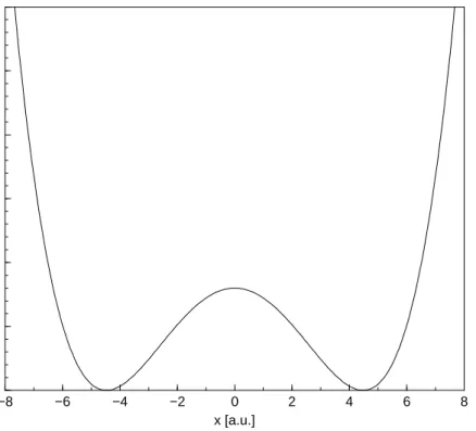
Let us first regard a symmetric double-minimum potential V(x) of the form (in atomic units)

V(x) = (0.2x4₋₈_x2₋₈₀₎_·₁₀−4_, _(4.1)

which is displayed in fig. 4.1. This potential form describes, e.g. the ammonia umbrella motion giving rise to the NH3 maser transitions [64]. Also, it often

serves as a model to characterize proton transfer processes taking place along a 46

(55)

CHAPTER 4. DYNAMICS IN DOUBLE WELL POTENTIALS 47

reaction coordinatex [57, 65–67]. Regarding, e.g. a particle localized in the well

−8 −6 −4 −2 0 2 4 6 8 x [a.u.] 0 0.005 0.01 0.015 0.02 0.025 0.03 V(x) [a.u.]

Figure 4.1: Potential energy surface of the generic double minimum potential. at positive values of x, the objective is to move it over the potential barrier and stabilize it in the inner well, at least for times which are smaller than the time-scale where tunneling occurs. Therefore a heating fieldEh(t) is employed as long as the particle’s coordinate is smaller than the position of the potential barrier. As soon as it has reached negative values ofxthe field is to be phase-shifted and exhibits the form of a cooling field Ec(t).

4.1.1

Classical Trajectories

In the classical picture a trajectory, starting at pointx0 = 5.1 a.u. with an initial

velocity ˙x= 0, was propagated using the Runge-Kutta algorithm. For a particle with proton mass m and a linear dipole moment µ(x) = 0.2x+ 1 a.u. the field

(56)

48 4.1. ONE-DIMENSIONAL CASES was determined as E(t) =E0 ˙ x(t) m {Θ[−x(t)]−Θ[x(t)]} (4.2) where Θ denotes the Heaviside step function. This means that, if the particle’s position is inside the starting well a heating occurs, whereas, if it exceeds the barrier, a cooling sets in. To facilitate a comparison to a quantum dynamical cal-culation an ensemble of 50 trajectories was propagated, weighted with a Gaussian distribution Pi of the form

Pi(x) =e−6·(xi−xc)2_, _(4.3)

where i counts the trajectories. In order to compare classical dynamics with the quantum dynamics the Gaussian was chosen to exhibit the same extent as a quantum mechanical wave function. The classical density is then constructed from the ensemble each at a pointxi, weighted with the Gaussian distributionPi for the particular trajectory i

ρ=X

i

Pixi. (4.4)

The xi were chosen to be centered around a value xc= 5.1 a.u. according to the position where the quantum machanical wave packet is centered. Applying the Runge-Kutta algorithm

ρ12(t) = ρ0+ ∆tx˙0_i

(57)

CHAPTER 4. DYNAMICS IN DOUBLE WELL POTENTIALS 49 0 100 200 300 400 500 600 700 800 900 1000-10 -8 -6 -4 -2 0 2 4 6 8 10 x [a.u.] Time [fs]

Figure 4.2: Dynamics of the classical density in the double minimum potential. The initially localized trajectory ensemble in the outer potential well is transferred over the barrier and stabilized in the inner well.

where the velocities ˙xi were weighted with the quantum mechanical momentum distributionPi,mom, likewise assumed to be of Gaussian form

Pi,mom( ˙x) = e−0.3·( ˙xi−p0)

2

(4.6) ˙

xi = x˙iPi,mom. (4.7)

The momentum distribution is centered around p0 = 0, meaning that the most

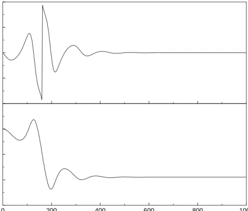
probable momentum is zero. The field resulting from eq. (4.2) driving the dy-namics (fig. 4.2) is presented in fig. 4.3 where we used a value of E0 = 8·10−4

a.u.. It can be seen that the transition is possible during the second vibrational period. Afterwards the cooling sets in and stabilizes the trajectory ensemble. The constructed electric field shows the temporal behaviour as described in chapter 3.

(58)

50 4.1. ONE-DIMENSIONAL CASES 0 200 400 600 800 1000 Time [fs] −10 −5 0 5 x [a.u.] −0.01 −0.005 0 0.005 0.01 I [a.u.]

Figure 4.3: Upper panel: Electric field constructed from the momentum changes in the classical system. The phase jump results from the Heaviside step function, occuring at the time where the ensemble average value _hx_i of the trajectory ensemble displayed in the lower panel equals zero.

4.1.2

Quantum Dynamical Picture

Applying the algorithm of instantaneous control to the quantum dynamics, a field can be constructed in analogy to the classical procedure by replacing in eq. (4.2) the classical ensemble average value by the quantum mechanical expectation value. Therefore an initial Gaussian wave function centered aroundxc= 5.1 a.u. with a width of 2 a.u. was employed and the dipole moment was chosen as in the classical treatment. A comparable dynamics was procured with a value of E0 = 1·10−5. The wave packet dynamics and the corresponding field are shown

(59)

CHAPTER 4. DYNAMICS IN DOUBLE WELL POTENTIALS 51 x [a.u.] 0 100 200 300 400 500 600 700 800 900 1000 Time [fs] -8 -6 -4 -2 0 2 4 6 8 x [au] 0 100 200 300 400 500 600 700 800 900 1000 Time [fs] -8 -6 -4 -2 0 2 4 6 8

Figure 4.4: Wave packet dynamics in the double minimum potential. The initially localized wave packet in the outer potential well is transferred over the barrier and stabilized in the inner well.

The fields derived from the classical and the quantum mechanical description are similar. We tried to insert the classical field into the quantum dynamical calculations in order to examine the conduct of the quantized system. The result is pictured in fig. 4.6. It can bee seen that the population transfer is not complete, a part of the wave packet has too much energy and re-crosses the barrier. At the time when the cooling process sets in, two parts are cooled down in the particular well. The quantum dynamical behaviour can not be expressed completely in terms of classical mechanics.

(60)

52 4.1. ONE-DIMENSIONAL CASES 0 200 400 600 800 Time [fs] −0.01 −0.005 0 0.005 0.01 I [a.u.]

Figure 4.5: Electric field constructed from the momentum changes in the system. The phase jump results from the Heaviside step function, occuring at the time where the bond-length expectation value _hx_i of the wave packet equals zero.

4.1.3

Asymmetric Double-Well Potential

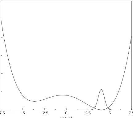
In what follows, the over-the-barrier dynamics in an asymmetric double-well po-tential is examined. Its analytical form is given as (in atomic units)

V(x) = (0.5x4₋1_·10−5_x3

<

Laser-Control of Molecular Dynamics. Dissertation