PRISM: A Prime-Encoding Approach for Frequent Sequence Mining
Karam Gouda
∗, Mosab Hassaan
∗, Mohammed J. Zaki
† ∗Mathematics Dept., Faculty of Science, Benha, Egypt
†Department of Computer Science, RPI, Troy, NY, USA
karam [email protected], mosab [email protected], [email protected]
Abstract
Sequence mining is one of the fundamental data mining tasks. In this paper we present a novel approach called
PRISM, for mining frequent sequences. PRISM utilizes a vertical approach for enumeration and support counting,
based on the novel notion ofprime block encoding, which in
turn is based on prime factorization theory. Via an extensive evaluation on both synthetic and real datasets, we show that
PRISMoutperforms popular sequence mining methods like SPADE [10], PrefixSpan [6] and SPAM [2], by an order of magnitude or more.
1
Introduction
Many real world applications, such as in bioinformatics, web mining, text mining and so on, have to deal with se-quential/temporal data. Sequence mining helps to discover frequent sequential patterns across time or positions in a given data set. Mining frequent sequences is one of the basic exploratory mining tasks, and has attracted a lot of attention [1, 2, 4–6, 9, 10].
Problem Definition: The problem of mining sequential
patterns can be stated as follows: LetI ={i1, i2,· · ·, im} be a set ofmdistinct attributes, also calleditems. An item-setis a non-empty unordered collection of items (without loss of generality, we assume that items of an itemset are sorted in increasing order). Asequenceis an ordered list of itemsets. An itemsetiis denoted as(i1i2· · ·ik), whereij
is an item. An itemset with kitems is called a k-itemset. A sequence S is denoted as (s1 → s2 → · · · → sq), where eachelementsj is an itemset. The number of item-sets in the sequence gives itssize(q), and the total number of items in the sequence gives itslength(k=j|sj|). A sequence of lengthk is also called ak-sequence. For ex-ample, (b → ac) is a 3-sequence of size 2. A sequence S = (s1→ · · · →sn)is asubsequenceof (or iscontained
in) another sequenceR = (r1 → · · · →rm), denoted as S ⊆R, if there exist integersi1 < i2<· · ·< insuch that sj ⊆rij for allsj. For example the sequence(b →ac)is a subsequence of(ab →e →acd), but(ab → e)is not a subsequence of(abe), and vice versa.
Given a databaseDof sequences, each having a unique sequence identifier, and given some sequenceS = (s1 → · · · → sn), the absolute supportof S inD is defined as the total number of sequences in Dthat containS, given as sup(S,D) = |{Si ∈ D|S ⊆ Si}|. The relative sup-port of S is given as the fraction of database sequences
that containS. We use absolute and relative supports in-terchangeably. Given a user-specified threshold called the
minimum support(denotedminsup), we say that a sequence
isfrequent if occurs more thanminsup times. A frequent
sequence ismaximalif it is not a subsequence of any other frequent sequence. A frequent sequence isclosedif it is not a subsequence of any other frequent sequence with the same support. Given a databaseDof sequences andminsup, the problem of mining sequential patterns is to find all frequent sequences in the database.
Related Work:The problem of mining sequential patterns
was introduced in [1]. Many other approaches have fol-lowed since then [2, 4–10]. Sequence mining is essentially an enumeration problem over the sub-sequence partial order looking for those sequences that are frequent. The search can be performed in a breadth-first or depth-first manner, starting with more general (shorter) sequences and extend-ing them towards more specific (longer) ones. The existextend-ing methods essentially differ in the data structures used to “in-dex” the database to facilitate fast enumeration. The exist-ing methods utilize three main approaches to sequence min-ing: horizontal [1, 5, 7], vertical [2, 4, 10] and projection-based [6, 9].
Our Contributions: In this paper we present a novel
ap-proach called PRISM (which stands for the bold letters in: PRIme-Encoding Based Sequence Mining) for min-ing frequent sequences. PRISMutilizes a vertical approach for enumeration and support counting, based on the novel notion of prime block encoding, which in turn is based on prime factorization theory. Via an extensive evalu-ation on both synthetic and real datasets, we show that PRISMoutperforms popular sequence mining methods like SPADE [10], PrefixSpan [6] and SPAM [2], by an order of magnitude or more.
2
Preliminary Concepts
Prime Factors & Generators: An integerpis aprime
in-teger if p > 1 and the only positive divisors ofp are 1
andp. Every positive integer n is either 1 or can be ex-pressed as a product of prime integers, and this factoriza-tion is unique except for the order of the factors [3]. Let p1, p2,· · ·, prbe the distinctprime factors ofn, arranged in order, so thatp1 < p2 < · · · < pr. All repeated fac-tors can be collected together and expressed using expo-nents, so that n = pm1
1 pm22· · ·pmrr, where eachmi is a
factor-ization ofnis called thestandard formofn. For example, n= 31752 = 23·34·72.
Given two integersa=ri=1a pmia
ia andb =
rb
i=1pmibib
in their standard forms, the greatest common divisor of the two numbers is given as gcd(a, b) = ipmi
i , where
pi = pja = pkb is a factor common to bothaandb, and mi = min(mja, mkb), with1 ≤ j ≤ ra,1 ≤ k ≤ rb. For example, ifa= 7056 = 24·32·72andb= 18900 = 22·33·52·7, thengcd(a, b) = 22·32·7 = 252.
For our purposes, we are particularly interested in
square-freeintegersn, defined as integers, whose prime
fac-torspiall have multiplicitymi= 1(note: the name square-free suggests that no multiplicity is 2 or more, i.e., the num-ber does not contain a square of any factor). Given a setG, letP(G)denote the set of all subsets ofG. If we assume that G is ordered and indexed by the set {1,2,· · · ,|G|}, then any subset S ∈ P(G)can be represented as a |G |-length bit-vector (or binary vector), denotedSB, whosei -th bit (from left) is 1 if -the i-th element of Gis inS, or else thei-th bit is 0. For example, ifG={2,3,5,7}, and S={2,5}, thenSB= 1010.
Given a set S ∈ P(G), we denote by ⊗S, the value obtained by applying the multiplication operator ⊗to all members ofS, i.e.,⊗S=s1·s2·. . .·s|S|, withsi∈S. If S =∅, define⊗S = 1. Let⊗P(G) ={⊗S:S ∈P(G)} be the set obtained by applying the multiplication operator on all sets in P(G). In this case we also say thatG is a
generatorof⊗P(G)under the multiplication operator.
We say that a set Gis asquare-free generator if each X ∈ ⊗P(G)is square-free. In case a generatorGconsists of only prime integers, we call it aprime generator. Recall that asemi-groupis a set that is closed under an associative binary operator⊗. We say that a setPis asquare-free
semi-groupiff for allX, Y ∈ P, ifZ = X⊗Y is square-free,
thenZ∈P.
Theorem 2.1 A setP is a square-free semi-group with
op-erator⊗iff it has a square-free prime generatorG. In other
words,Pis a square-free semi-group iffP=⊗P(G).
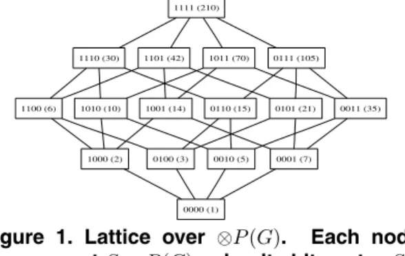
As an example, let G = {2,3,5,7} be the set of the first four prime numbers. Then ⊗P(G) = {1,2,3,5,7,6,10,14,15,21,35,30,42,70,105,210}. It is easy to see that G is a square-free generator of⊗P(G), which in turn is a square-free semi-group, since the prod-uct of any two of its elements that is square-free is already in the set. 1111 (210) 1110 (30) 1101 (42) 1011 (70) 0111 (105) 1100 (6) 1010 (10) 1001 (14) 0110 (15) 0101 (21) 0011 (35) 1000 (2) 0100 (3) 0010 (5) 0001 (7) 0000 (1)
Figure 1. Lattice over ⊗P(G). Each node shows a setS∈P(G)using its bit-vectorSB and the value obtained by multiplying its ele-ments⊗S.
The set P(G) induces a lattice over the semi-group ⊗P(G) as shown in Figure 1. In this lattice, the meet
operation (∧) is set intersection over elements of P(G),
which corresponds to the gcd of the corresponding ele-ments of⊗P(G). Thejoin operation (∨)is set union (over P(G)), which corresponds to the least common multiple
(lcm)over⊗P(G). For example,1010(10)∧1001(14) =
1000(2), confirming thatgcd(10,14) = 2, and1010(10)∨
1001(14) = 1011(70), indicating thatlcm(10,14) = 70. More formally, we have:
Theorem 2.2 Let⊗P(G)be a square-free semi-group with
prime generator G, and let X, Y ∈ ⊗P(G)be two
dis-tinct elements, then gcd(X, Y) = ⊗(SX ∩ SY), and
lcm(X, Y) = ⊗(SX ∪SY), whereX = ⊗SX andY =
⊗SY, andSX, SY ∈P(G)are the prime factors ofXand
Y, respectively.
Define thefactor-cardinality, denotedXG, for anyX ∈ ⊗P(G), as the number of prime factors fromGin the fac-torization of X. Let X = ⊗SX, withSX ⊆ G. Then XG = |SX|. For example,21G ={3,7} = 2. Note that{1}G= 0, since1has no prime factors inG.
Corollary 2.3 Let ⊗P(G) be a square-free semi-group
with prime generator G, and letX, Y ∈ ⊗P(G) be two
distinct elements, thengcd(X, Y)∈ ⊗P(G).
Prime Block Encoding:LetT = [1 :N] ={1,2, . . . , N}
be the set of the first N positive integers, letGbe a base set of prime numbers sorted in increasing order. Without loss of generality assume thatN is a multiple of|G|, i,.e., N =m· |G|. LetB∈ {0,1}N be a bit-vector of lengthN. ThenB can partitioned intom = |NG| consecutive blocks, where each blockBi=B[(i−1)· |G|+ 1 : i· |G|], with
1 ≤i ≤ m. In fact, eachBi ∈ {0,1}|G|, is the indicator bit-vectorSBrepresenting some subsetS ⊆G. LetBi[j] denote thej-th bit inBi, and letG[j]denote thej-th prime inG. Define thevalueofBi with respect toGas follows, ν(Bi, G) =⊗{G[j]Bi[j]}. For example ifB
i = 1001, and
G={2,3,5,7}, thenν(Bi, G) = 21·30·50·71= 2·7 = 14. Note also that ifBi= 0000thenν(Bi, G) = 1.
Define ν(B, G) = {ν(Bi, G) : 1 ≤ i ≤ m}, as
the prime block encoding of B with respect to the base
prime set G. It should be clear that each ν(Bi, G) ∈ ⊗P(G). Note that when there is no ambiguity, we write ν(Bi, G) as ν(Bi), andν(B, G) as ν(B). As an exam-ple, let T = {1,2, ...,12}, G = {2,3,5,7}, and B = 100111100100. Then there are m = 12/4 = 3 blocks, B1 = 1001, B2 = 1110 and B3 = 0100. We have ν(B1) = ⊗SG(B1) = ⊗{2,7} = 2·7 = 14, and the prime block encoding ofBis given asν(B) ={14,30,3}. We also define the inverse operation ν−1({14,30,3}) = ν−1(14)ν−1(30)ν−1(3) = 100111100100 = B. Also a bit-vector of all zeros (of any length) is denoted as0, and its corresponding value/encoding is denoted as1. For ex-ample, ifC = 00000000, then we also writeC = 0, and ν(C) ={1,1}=1.
LetGbe the base prime set, and letA=A1A2· · ·Am, andB =B1B2· · ·Bmbe any two bit-vectors in{0,1}N, with N = m · |G|, and Ai, Bi ∈ {0,1}|G|. De-fine gcd(ν(A), ν(B)) = {gcd(ν(Ai), ν(Bi)) : 1 ≤
i ≤ m}. For example, for ν(B) = {14,30,5} and ν(A) = {2,210,2}, we have gcd(ν(B), ν(A)) = {gcd(14,2), gcd(30,210), gcd(5,2)}={2,30,1}.
Let A = A1A2· · ·Am be a bit-vector of length N, where each Ai is a |G| length bit-vector. Let fA = arg minj{A[j] = 1}be the position of the first ‘1’ in A, across all blocks Ai. Define a maskingoperator (A) as follows:
(A)[j] =
0, j≤fA 1, j > fA
In other words, (A) is the bit vector obtained by set-ting A[fA] = 0 and setting A[j] = 1 for all j > fA. For example, if A = 001001100100, then fA = 3, and (A) = 000111111111. Likewise, we can define the masking operator for a prime block encod-ing as follows: (ν(A)) = ν((A)). For example,
(ν(A)) = ν((001001100100)) = ν(000111111111) = ν(0001) ν(1111) ν(1111) = {7,210,210}. In other words, ({5,15,3}) = {7,210,210}, since ν(A) = ν(001001100100) = ν(0010) ν(0110) ν(0100) = {5,15,3}.
3
The
PRISM
Algorithm
Sequence mining involves a combinatorial enumeration or search for frequent sequences over the sequence partial order. There are three key aspects of PRISM that need elucidation: i) the search space traversal strategy, ii) the data structures used to represent the database and interme-diate candidate information, and iii) how support counting is done for candidates. PRISMuses the prime block encod-ing approach to represent candidates sequences, and uses join operations over the prime blocks to determine the fre-quency for each candidate.
Search Space: The partial order induced by the
subse-quence relation is typically represented as a search tree, de-fined recursively as follows: The root of the tree is at level zero and is labeled with the null sequence ∅. A node la-beled with sequenceS at levelk, i.e., ak-sequence, is re-peatedly extended by adding one item fromIto generate a child node at the next level (k+ 1), i.e., a(k+ 1)-sequence. There are two ways to extend a sequence by an item:
se-quence extensionanditemset extension. In a sequence
ex-tension, the item is appended to the sequential pattern as a new itemset. In an itemset extension, the item is added to the last itemset in the pattern, provided that the item is lexicographically greater than all items in the last itemset. Thus, a sequence-extension always increases the size of the sequence, whereas, an itemset-extension does not. For ex-ample, if we have a nodeS = ab → aand an itembfor extendingS, then ab → a → b is a sequence-extension, andab→abis an itemset extension.
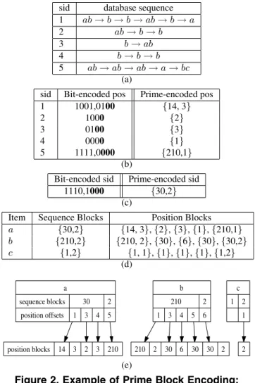
Prime Block Encoding: Consider the example database
in Figure 2(a), consisting of 5 sequences over the items I = {a, b, c}. Let G = {2,3,5,7} be the base square-free prime generator set. Let’s see how PRISM constructs the prime block encoding for a single itema. In the first step, PRISMconstructs the prime encoding of the positions within each sequence. For example, sinceaoccurs in po-sitions 1,4, and 6 (assuming popo-sitions/indexes starting at 1) in sequence 1, we obtain the bit-encoding ofa’s
occur-sid database sequence 1 ab→b→b→ab→b→a 2 ab→b→b 3 b→ab 4 b→b→b 5 ab→ab→ab→a→bc (a)
sid Bit-encoded pos Prime-encoded pos 1 1001,0100 {14, 3} 2 1000 {2} 3 0100 {3} 4 0000 {1} 5 1111,0000 {210,1} (b)
Bit-encoded sid Prime-encoded sid 1110,1000 {30,2}
(c)
Item Sequence Blocks Position Blocks a {30,2} {14, 3},{2},{3},{1},{210,1} b {210,2} {210, 2},{30},{6},{30},{30,2} c {1,2} {1, 1},{1},{1},{1},{1,2} (d) a sequence blocks position offsets 30 1 3 4 2 5 position blocks 14 3 2 3 210 b 210 1 3 4 5 2 6 210 2 30 6 30 30 2 c 1 2 1 2 (e)
Figure 2. Example of Prime Block Encoding: (a) Example Database. (b) Position Encoding fora. (c) Sequence Encoding for a. (d) Full Prime Blocks fora, b andc. (e) Prime Block Encoding fora,bandc.
rences: 100101. PRISM next pads this bit-vector so that it is a multiple of |G| = 4, to obtain A = 10010100 (note: bold bits denote padding). Next we computeν(A) = ν(1001)ν(0100) = {14,3}. The position encoding for a over all the sequences is shown in Figure 2 (b).
PRISM next computes the prime encoding for the se-quence ids. Sinceaoccurs in all sequences, except for 4, we can representa’s sequence occurrences as a bit-vector A= 11101000after padding. This yields the prime encod-ing shown in Figure 2(c), sinceν(A) =ν(1110)ν(1000) = {30,2}. The full prime encoding for itemaconsists of all the sequence and position blocks, as shown in Figure 2(d). A blockAi = 0000 = 0, withν(Ai) = {1} =1, is also called anemptyblock. Note that the full encoding retains all the empty position blocks, for example,adoes not occur in the second position block in sequence 5, and thus its bit-vector is0000, and the prime code is{1}. In general, since items are expected to be sparse, there may be many blocks within a sequence where an item does not appear.
To eliminate those empty blocks, PRISMretains only the non-empty blocks in the prime encoding. To do this it needs
to keep an index with each sequence block to indicate which non-empty position blocks correspond to a given sequence block. Figure 2 (e) shows the actual (compact) prime block encoding for itema. The first sequence block is 30, with factor-cardinality30G = 3, which means that there are 3 valid (i.e., with non-empty position blocks) sequences in this block, and for each of these, we store the offsets into the position blocks. For example, the offset of sequence 1 is 1, with the first two position blocks corresponding to this sequence. Thus the offset for sequence 2 is 3, with only one position block, and finally, the offset of sequence 3 is 4. Note that the sequences which represent the sequence block 30, can be found directly from the corresponding bit-vector ν−1(30) = 1110, which indicates that sequence 4 is not valid. The second sequence block forais2 (corre-sponding toν−1(2) = 1000), indicating that only sequence 5 is valid, and its position blocks begin as position 5. The benefit of this sparse representation becomes clear when we consider the prime encoding for c. Its full encoding (see Figure 2(d)) contains a lot of redundant information, which has been eliminated in the compact prime block encoding (see Figure 2(e)).
It is worth noting that the support of a sequenceScan be directly determined from its sequence blocks in the prime block encoding. Let E(S) = (SS,PS) denote the prime block encoding for sequence S, where SS is the set of all encoded sequence blocks, and PS is the set of all en-coded position blocks forS. The support of a sequenceS with prime block encodingE(S) = (SS,PS) is given as sup(S) = vi∈SSviG. For example, forS =a, since Sa ={30,2}, we havesup(a) =30G+2G= 3+1 = 4. Given a list of full or compact position blocksPS for a sequenceS, we use the notationPSi to denote those posi-tions blocks, which come from sequence idi. For example, inPa1 ={14,3}. In the full encodingPa5 ={210,1}, but in the compact encodingPa5={210}(see Figure 2(d)-(e)).
Support Counting via Prime Block Joins: The frequent
sequence enumeration process starts with the root of the search tree as the prefix nodeP =∅, and PRISM assumes that initially we know the prime block encodings for all sin-gle items. PRISMthen recursively extends each node in the search tree, computes the support via the prime block joins, and retains new candidates (or extensions) only if they are frequent. The search is essentially depth-first, the main dif-ference being that for any nodeS, all of its extensions are evaluated before the depth-first recursive call. When there are no new frequent extensions found, the search stops. To complete the description, we now detail the prime block join operations. We will illustrate the prime block item-set and sequence joins using the prime encodingsE(a)and E(b), for items a and b, respectively, as shown in Fig-ure 2(e).
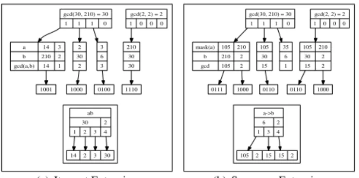
Itemset Extensions: Let’s first consider how to obtain the
prime block encoding for the itemset extension E(ab), which is illustrated in Figure 3(a). Note that the sequence blocks Sa = {30,2} and Sb = {210,2} contain all in-formation about the relevant sequence ids where a andb occur, respectively. To find the sequence block for item-set extension ab, we simply have to compute the gcdfor the corresponding elements from the two sequence blocks, namelygcd(30,210) = 30 (which corresponds to the
bit-gcd(30, 210) = 30 1 1 1 0 a b gcd(a,b) 14 210 14 3 2 1 2 30 2 3 6 3 1001 1000 0100 ab 30 1 2 3 2 4 gcd(2, 2) = 2 1 0 0 0 210 30 30 1110 14 2 3 30
(a) Itemset Extension
gcd(30, 210) = 30 1 1 1 0 mask(a) b gcd 105 210 105 210 2 2 105 30 15 35 6 1 0111 1000 0110 a->b 6 1 3 2 4 gcd(2, 2) = 2 1 0 0 0 105 30 15 210 2 2 0110 1000 105 2 15 15 2 (b) Sequence Extension Figure 3. Extensions via Prime Block Joins vector1110), andgcd(2,2) = 2(which corresponds to bit-vector1000). We say that a sequence id i ∈ gcd(Sa,Sb) if the i-th bit is set in the bit vector ν−1(gcd(Sa,Sb)). Since ν−1(gcd(Sa,Sb)) = ν−1({30,2},{210,2}) = ν−1(30,2) = 11101000, we find that sids 1, 2, 3 and 5 are the ones that contain occurrences of bothaandb.
All that remains to be done is to determine, by looking at the position blocks, ifaandb, in fact, occur simultane-ously at some position in those sequences. Let’s consider each sequence separately. Looking at sequence 1, we find in Figure 2(e) that its positions blocks are Pa1 = {14,3} in E(a) and Pb1 = {210,2} in E(b). To find where a and b co-occur in sequence 1, all we have to do is com-pute thegcdof these position blocks to obtaingcb(a, b) = {gcd(14,210), gcd(3,2)} = {14,1}, which indicates that ab only occur at positions 1 and 4 in sequence 1 (since ν−1(14) = 1001). A quick look at Figure 2(a) confirms that this is indeed correct. If we continue in like manner for the remaining sequences (2, 3 and 5), we obtain the re-sults shown in Figure 3(a), which also shows the final prime block encodingE(ab). Note that there is at least one non-empty block for each of the sequences, even though for se-quence 1, the second position block is discarded in the final prime encoding. Thussup(ab) =30G+2G= 3+1 = 4.
Sequence Extensions: Let’s consider how to obtain the
prime block encoding for the sequence extensionE(a→b), which is illustrated in Figure 3(b). The first step involves computing thegcdfor the sequence blocks as before, which yields sequences 1, 2, 3 and 5, as those which may poten-tially contain the sequencea→b.
For sequence 1, we have the positions blocks P1
a = {14,3} for a and Pb1 = {210,2} for
b. The key difference with the itemset extension is the way in which we process each sequence. In-stead of computing gcd({14,3},{210,2}), we compute gcd(({14,3}),{210,2}) = gcd({105,210},{210,2}) = {gcd(105,210), gcd(210,2)} = {105,2}. Note that ν−1({105,2}) = 01111000, which precisely indicate those positions in sequence 1, whereboccurs after ana. Thus, sequence joins always keep track of the positions of the last item in the sequence. Proceeding in like manner for sequences 2,3, and 5, we obtain the results shown in Fig-ure 3(b). Note that for sequence 3, even though it contains both itemsaandb,bnever occurs after ana, and thus se-quence 3 does not contribute to the support ofa→b. This is also confirmed by computinggcd((3),6) =gcd(35,6) =
1, which leads to an empty block (ν−1(1) = 0000). Thus in the compact prime encoding of E(a → b), sequence 3 drops out. The remaining sequences 1, 2, and 5, con-tribute at least one non-empty block, which yieldsSa→b = ν(11001000) = {6,2}, as shown in Figure 3(b), with sup-portsup(a→b) =6G+2G = 2 + 1 = 3.
Optimizations: Since computing thegcd is one of main
operations in PRISM, we use a pre-computed table called GCDto facilitate rapidgcdcomputations. Note that in our examples above, we used only the first four primes as the base generator set G. However, in our actual implemen-tation, we used|G| = 8 primes as the generator set, i.e., G = {2,3,5,7,11,13,17,19}. Thus each block size is now 8 instead of 4. Note that with the newG, the largest element in ⊗P(G)is⊗G = 9699690. In total there are | ⊗P(G)|= 256possible elements in semi-group⊗P(G). In a naive implementation, the GCD lookup table can be stored as a two-dimensional array with cardinality
9699690×9699690, whereGCD(i, j) =gcd(i, j)for any two integers i, j ∈ [1 : 9699690]. This is clearly grossly inefficient, since there are in fact only 256 distinct (square-free) products in ⊗P(G), and we thus really need a table of size256×256to store all thegcdvalues. We achieve this by representing each element in⊗P(G)by its rank, as opposed to its value.
Let S ∈ P(G), and let SB its |G|-length indicator bit-vector, whose i-th bit is ‘1’ iff the i-element of G is in S. Then the rank of ⊗S is equal to the decimal value ofSB(with the left-most bit being the least signif-icant bit). In other words rank(⊗S) = decimal(SB). For example, the rank(1) = decimal(00000000) = 0, rank(13) = decimal(00000100) = 32, rank(35) = decimal(00110000) = 12, and rank(9699690) = decimal(11111111) = 255. LetS, T ∈ P(G), and let SB, TBbe their indicator bit-vectors with respect to gener-ator setG. Thenrank(gcd(⊗S,⊗T)) = decimal(SB∧ TB). Consider for example, gcd(35,6) = 1. We have rank(gcd(35,6)) = decimal(00110000∧11000000) = decimal(00000000) = 0, which matches the computation rank(gcd(35,6)) = rank(1) = 0. Instead of using di-rect values, all gcd computations are performed in terms of the ranks of the corresponding elements. Thus each cell in the GCD table stores: GCD(rank(i), rank(j)) = rank(gcd(i, j)), wherei, j ∈ ⊗P(G). This brings down the storage requirements of the GCDtable to just256×
256 = 65536bytes, since eachrankrequires only one byte of memory (sincerank∈[0 : 255]).
Once the final sequence blocks are computed for af-ter a join operation, we need to deaf-termine the actual sup-port, by adding the factor cardinalities for each sequence block. To speed up this support determination, PRISM maintains a one-dimensional look-up array calledCARD to store the factor-cardinality for each element in the set ⊗P(G). That is we storeCARD(rank(x)) = xG for allx∈ ⊗P(G). For example, since35G = 2, we have
CARD(rank(35)) =CARD(12) = 2.
Furthermore, in sequence block joins, we need to com-pute the masking operation for each position block. For this PRISMmaintains another one dimensional array called M ASK, where M ASK(rank(x)) = rank((x)) for each x ∈ ⊗P(G). For example M ASK(rank(2)) =
rank((2)) = rank(4849845) = 254. Finally, as an optimization for fast joins, once we determine gcdXY or gcdX→Y in the prime itemset/sequence block joins, if the number of supporting sequences is less thanminsup, we can stop further processing of position blocks, since the result-ing extensions cannot be frequent in this case.
4
Experiments
In this section we study the performance of PRISM by varying different database parameters and by comparing it with other state-of-the-art sequence mining algorithms like SPADE [10], PrefixSpan [6] and SPAM [2]. The codes/executables for these methods were obtained from their authors. All experiments were performed on a lap-top with 2.4GHz Intel Celeron processor, and with 512MB memory, running Linux.
Synthetic and Real Datasets: We used several synthetic
datasets, generated using the approach outlined in [1]. The datasets are generated using the following process. FirstNI maximal itemsets of average size I are generated by choos-ing from N items. ThenNS maximal sequences of average size S are created by assigning itemsets from NI to each sequence. Next a customer (or input sequence) of aver-age C transactions (or itemsets) is created, and sequences inNSare assigned to different customer elements, respect-ing the average transaction size of T. The generation stops when D input-sequences have been generated. For example, the datasetC20T50S20I10N1kD100k, means that it has D=100k sequences, with C=20 average transactions, T=50 average transaction size, chosen from a pool with average sequence size S=20 and average transaction size I=10, with N=1k different items. The default itemset and sequence pool sizes are always set toNS = 5000andNI = 25000, respectively.
We also compared the methods on two real datasets taken from [9]. Gazelle was part of the KDD Cup 2000 challenge dataset. It contains log data from a (de-funct) web retailer. It has 59602 sequences, with an av-erage length of 2.5, length range of [1, 267], and 497 distinct items. The Protein dataset contains 116142 proteins sequences downloaded from the Entrez database at NCBI/NIH. The average sequence length is 482, with length range of [400,600], and 24 distinct items (the dif-ferent amino acids).
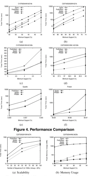
Performance Comparison: Figure 4 shows the
per-formance comparison of the four algorithms, namely, SPAM [2], PrefixSpan [6], SPADE [10] and PRISM, on different synthetic and real datasets, with varying mini-mum support. As noted earlier, for PRISM we used the first 8 primes as the base prime generator set G. Fig-ure 4 (a)-(b) show (small) datasets where all four meth-ods can run for at least some support values. For these datasets, we find that PRISM has the best overall perfor-mance. For the support values where SPAM can run, it is generally in the second spot (in fact, it is the fastest on
C10T20S4I4N0.1kD10k). However, SPAM fails to run for lower support values. PRISM outperforms SPADE by about 4 times, and PrefixSpan by over an order of magni-tude.
Figure 4 (c)-(d) show larger datasets (with D=100k se-quences). On these SPAM could not run on our laptop, and
10 100 1000 10000 35 40 45 50 55 60
Total Time (sec)
Minimum Support (%) C10T60S4I4N1kD10k Spam PrefixSpan Spade PRISM (a) 1 10 100 1000 10000 74 76 78 80 82 84 86 88 90
Total Time (sec)
Minimum Support (%) C35T40S20I20N1kD1k Spam PrefixSpan Spade PRISM (b) 100 150 200 250 300 350 400 450 500 550 600 3 3.5 4 4.5 5
Total Time (sec)
Minimum Support (%) C10T20S20I10N1kD100k PrefixSpan Spade PRISM (c) 10 100 1000 10000 95 95.5 96 96.5 97 97.5 98
Total Time (sec)
Minimum Support (%) C20T20S20I10N0.1kD100k PrefixSpan Spade PRISM (d) 1 10 100 1000 10000 0.055 0.057 0.059
Total Time (sec)
Minimum Support (%) Gazelle PrefixSpan Spade PRISM (e) 100 1000 10000 99.97 99.98 99.99
Total Time (sec)
Minimum Support (%) Protein Spade
PRISM
(f) Figure 4. Performance Comparison
10 100 1000
10 20 30 40 50 60 70 80 90 100
Total Time (sec)
Number of Sequences D (in 1000s; minsup = 30%) C20T20S20I10N1kD?k PrefixSpan Spade PRISM (a) Scalability 10 100 1000 10000 94 95 96 97 98 99
Peak Memory Usage (MB)
Minimum Support (%) C20T50S4I4N0.5kD5k Spam PrefixSpan Spade PRISM (b) Memory Usage Figure 5. Scalability & Memory Consumption thus is not shown. PRISM again outperforms PrefixSpan and SPADE, by up to an order of magnitude. Finally, Fig-ure 4 (e)-(f) show the performance comparison on the real datasets, Gazelleand Protein. SPAM failed to run on both these datasets on our laptop, and PrefixSpan did not run onProtein. OnGazellePRISMis an order of mag-nitude faster than PrefixSpan, but is comparable to SPADE. OnProtein PRISMoutperforms SPADE by an order of magnitude (for lower support).
Based on these results on diverse datasets, we can ob-serve some general trends. Across the board, our new approach, PRISM, is the fastest (with a few exceptions), and runs for lower support values than competing methods. SPAM generally works only for smaller datasets due to its very high memory consumption (see below); when it runs,
SPAM is generally the second best. SPADE and PrefixSpan do not suffer from the same problems as SPAM, but they are much slower than PRISM, or they fail to run for lower support values, when the database parameters are large.
Scalability: Figure 5(a) shows the scalability of the
differ-ent methods when we vary the number of sequences 10k to 100k (using as base values: C=20, T=20, S=20, I=10, and N=1k). Since SPAM failed to run on these larger datasets, we could not report on its scalability. We find that the ef-fect of increasing the number of sequences is approximately linear.
Memory Usage:Figure 5(b) shows the memory
consump-tion of the four methods on a sample of the datasets. The figures plot the peak memory consumption during execution (measured using thememusagecommand in Linux). Fig-ure 5(b) quickly demonstrates why SPAM is not able to run on all except very small datasets. We find that its memory consumption is well beyond the physical memory available (512MB), and thus the program aborts when the operating system runs out of memory. We can also note that SPADE generally has a 3-5 times higher memory consumption than PrefixSpan and PRISM. The latter two have comparable and very low memory requirements.
Conclusion: Based on the extensive experimental
compar-ison with popular sequence mining methods, we conclude that, across the board, PRISM is one of the most efficient methods for frequent sequence mining. It outperforms ex-isting methods by an order of magnitude or more, and has a very low memory footprint. It also has good scalability with respect to a number of database parameters. Future work will consider the tasks of mining all the closed and maximal frequent sequences, as well as the task of pushing constraints within the mining process to make the method suitable for domain-specific sequence mining tasks. For example, allowing approximate matches, allowing substi-tution costs, and so on.
References
[1] R. Agrawal and R. Srikant. Mining sequential patterns. In 11th ICDE Conf., 1995.
[2] J. Ayres, J. E. Gehrke, T. Yiu, and J. Flannick. Sequential pattern mining using bitmaps. InSIGKDD Conf., 2002. [3] J. Gilbert and L. Gilbert.Elements of Modern Algebra. PWS
Publishing Co., 1995.
[4] H. Mannila, H. Toivonen, and I. Verkamo. Discovering fre-quent episodes in sequences. InSIGKDD Conf., 1995. [5] F. Masseglia, F. Cathala, and P. Poncelet. The PSP approach
for mining sequential patterns. InEuropean PKDD Conf., 1998.
[6] J. Pei, J. Han, B. Mortazavi-Asl, H. Pinto, Q. Chen, U. Dayal, and M.-C. Hsu. Prefixspan: Mining sequential patterns efficiently by prefixprojected pattern growth. In ICDE Conf., 2001.
[7] R. Srikant and R. Agrawal. Mining sequential patterns: Gen-eralizations and performance improvements. InIntl. Conf. Extending Database Technology, 1996.
[8] J. Wang and J. Han. Bide: Efficient mining of frequent closed sequences. InICDE Conf., 2004.
[9] Z. Yang, Y. Wang, and M. Kitsuregawa. Effective sequential pattern mining algorithms for dense database. InJapanese Data Engineering Workshop (DEWS), 2006.
[10] M. J. Zaki. SPADE: An efficient algorithm for mining fre-quent sequences. Machine Learning Journal, 42(1/2):31– 60, Jan/Feb 2001.