Online Kernel Selection: Algorithms and Evaluations
Tianbao Yang
1, Mehrdad Mahdavi
1, Rong Jin
1, Jinfeng Yi
1, Steven C. H. Hoi
2 1Department of Computer Science and Engineering, Michigan State University, MI, 48824, USA2School of Computer Engineering, Nanyang Technological University, 639798, Singapore 1{yangtia1, mahdavim, rongjin, yijinfen}@msu.edu,2[email protected]
Abstract
Kernel methods have been successfully applied to many ma-chine learning problems. Nevertheless, since the performance of kernel methods depends heavily on the type of kernels be-ing used, identifybe-ing good kernels among a set of given ker-nels is important to the success of kernel methods. A straight-forward approach to address this problem is cross-validation by training a separate classifier for each kernel and choos-ing the best kernel classifier out of them. Another approach is Multiple Kernel Learning (MKL), which aims to learn a sin-gle kernel classifier from an optimal combination of multiple kernels. However, both approaches suffer from a high com-putational cost in computing the full kernel matrices and in training, especially when the number of kernels or the num-ber of training examples is very large. In this paper, we tackle this problem by proposing an efficient online kernel selection algorithm. It incrementally learns a weight for each kernel classifier. The weight for each kernel classifier can help us to select a good kernel among a set of given kernels. The pro-posed approach is efficient in that (i) it is an online approach and therefore avoids computing all the full kernel matrices before training; (ii) it only updates a single kernel classifier each time by a sampling technique and therefore saves time on updating kernel classifiers with poor performance; (iii) it has a theoretically guaranteed performance compared to the best kernel predictor. Empirical studies on image classifica-tion tasks demonstrate the effectiveness of the proposed ap-proach for selecting a good kernel among a set of kernels.
Introduction
Kernel methods have attracted a significant amount of in-terest in machine learning, computer vision, and bioinfor-matics due to their superior empirical performance. For a specific task in hand, many kernels can be applied based on the special characteristics of certain objects. For example, in image classification, various types of features can be ex-tracted (e.g. invariant SIFT features, bag-of-word features for images) and various types of kernels (e.g. chi-square, RBF, etc) can be used. As a result, the performance of kernel methods may depend on the kernel that is being used. It is empirically observed that in image classification, chi-square kernel is one of the most effective kernels (Zhang et al. 2007) and in text categorization, probability product kernel
Copyright c2012, Association for the Advancement of Artificial Intelligence (www.aaai.org). All rights reserved.
is a commonly used kernel which usually gives better per-formance than other kernels (Jebara, Kondor, and Howard 2004). Therefore, in the absence of prior experience, it is important to select an appropriate kernel for a specific task for the success of the kernel methods.
A straightforward approach for kernel selection is by cross-validation, i.e. training a separate kernel classifier for each individual kernel on a training data set and testing it on a separate validation data set, and then choosing the kernel classifier that gives the best performance on the validation data set. This approach wastes a lot of time on training, es-pecially for those very bad kernels.
An approach to avoid training individual kernel classifier for each kernel is by MKL, which aims to efficiently learn a single kernel classifier from a combination of the multiple kernels, where the combination weights are learned by min-imizing some empirical loss on a training data. However, MKL still suffers from a high computational cost in train-ing, and current algorithms for MKL do not scale very well to a large number of kernels or a large number of training examples. In addition, both approaches need to compute all the full kernel matrices before training.
In this work, we present an efficient online approach for kernel selection. It incrementally learns a weight for each kernel, which measures the relative importance of each ker-nel classifier for prediction, and selects a good kerker-nel based on the weights. The proposed approach is computationally efficient because it avoids computing all the full kernel ma-trices and updates a single kernel classifier each time by a sampling technique. The proposed approach also has a theo-retic guarantee in performance for the selected kernel com-pared to the best kernel. We refer to the proposed online leaning approach for selecting a good kernel asOnline Ker-nel Selection (OKS).
Related Work
The present work is closely related to model selection prob-lem. Model selection is the task of selecting a statisti-cal model from a set of candidate models, given training data. Many criteria and approaches have been proposed for model selection. Examples include AIC (Akaike 1974), BIC (Schwarz 1978), and Mallows’ Cp (Mallows 1973). Us-ing these criteria for model selection, one needs to train a model for each function class, computes the value of the
chosen criterion, and then selects the model that gives the best value. Another common practice for model selection is by cross-validation. The problem of these approaches is their high computational cost, i.e. one needs to learn a model completely for all function classes even though some classes may have very poor performance. Recently, Agarwal et al. (Agarwal et al. 2011) proposed an algorithm for model selection under a computational budget and proved its theo-retical guarantee. However, it makes an explicit assumption on the hierarchical structure of the functional classes. In our setting, we are facing a set of Reproducing Kernel Hilbert Spaces (RKHS), which do not satisfy the hierarchical struc-ture.
Our work is also related to kernel methods and kernel learning. Kernel methods have been used extensively in bioinformatics (Sch¨olkopf, Guyon, and Weston 2000), ma-chine learning (Sch¨olkopf and Smola 2001), and computer vision (Lampert 2009). An interesting question is to find the best kernel among a set of kernels for a specific task. A com-mon practice as we discussed before is by cross-validation. MKL is another approach to avoid training a separate model for each kernel. Many MKL algorithms have been pro-posed (Lanckriet et al. 2004; Rakotomamonjy et al. 2008; Xu et al. 2008; Cortes, Mohri, and Rostamizadeh 2010), to learn an optimal combination of kernels and the correspond-ing kernel classifier. However, these algorithms still suffer from high computational cost of computing the full kernel matrices and training as well.
The ideas used in the present paper draw on online learn-ing. In online learning, one needs to update the predictor incrementally given the examples are coming sequentially. Staring from Perceptron algorithm (Rosenblatt 1958), many online learning algorithms have been proposed (Crammer et al. 2006; Freund and Schapire 1997; Auer et al. 2003). Recently, several online MKL algorithms have been pro-posed (Orabona, Luo, and Caputo 2010; Jin, Hoi, and Yang 2010). Our work differs from these works in that we are not aiming to optimize multiple kernel learning in an online fashion. Instead, we are interested in quickly finding a good kernel among a set of kernels for prediction. Finally, we note that the our online kernel selection algorithm for classifica-tion (i.e. Algorithm 2) is similar to the single stochastic up-date algorithm in (Jin, Hoi, and Yang 2010), however, our framework (i) updates the weight vector based on exponen-tial weighted average algorithm, and (ii) uses an unbiased trick in updating the weight vector and the predictors, which together allow us to derive additive (rather than multiplica-tive) regret bound or mistake bound, and therefore to better compare with the performance of the best kernel.
We can summarize our contributions as follows: (i) we present a general online kernel selection algorithm for a pre-diction task with any convex loss function; (ii) we present an online kernel selection algorithm for classification with hinge loss; (iii) we present a theoretical analysis of the pro-posed algorithms for selecting a good kernel; (iv) we con-duct empirical evaluations on the proposed online kernel se-lection algorithms on image classification.
Online Kernel Selection
In this section, we present several online learning algorithms for online kernel selection. We first present a general on-line algorithm for any convex loss function, state its regret bound, and analyze its performance in selecting the best kernel. Then we present an algorithm for classification by adapting the general algorithm to hinge loss.
Before jumping to detailed algorithms, we first introduce some notations that will be used throughout the paper. We let(xt, yt)denote thetth example with feature
representa-tion xt ∈ Rd and labelyt, and let Km = {κ1,· · ·, κm}
denote the givenmkernels.Hκj denotes the Reproducing
Kernel Hilbert Space endowed byκj,fjt∈ Hκj denotes the
jth kernel predictor learned up totth trial,ft
j(xt)denotes its
evaluation on examplext, andft = (f1t,· · ·, f
t
m). We use
wt = (wt1,· · ·, wtm) ∈ Rm+ to denote the weights for the mkernel predictors learned up totth trial,qt=wt/Pjw
t j
to denote the normalized vector, andpt ∈ Rm+ to denote a probability vector, i.e.Pm
j=1p
t
j = 1. Let`(z, y)denote a
convex loss function with respect toz, and∇`(z, y)denote the (sub)gradient with respect toz. Finally,[m]denotes the set{1,· · ·, m}, andMulti(pt)denotes multinomial
distri-bution with parameterspt.
A General Algorithm and its Regret Bound
In this section, we present an online kernel selection algo-rithm for a general convex loss function, and state its regret bound. The basic steps of the proposed algorithm are shown in Algorithm 1. We explain the key steps of the algorithm in the following:
• Step 1:It takes as input a set of reproducing kernelsKm,
and parametersδ,η, λ.δis a smoothing parameter as ex-plained later.η, λare step sizes for updating the weights wtand the kernel predictorsft.
• Step 5:In trialt, after receiving one example(xt, yt), it
samples one kernel out by following a multinomial distri-bution parameterized bypt.
• Step 6:It updates the weight of the sampled kernel by ex-ponential weighted average algorithm, similar to predic-tion with expert advice (Cesa-Bianchi and Lugosi 2006). If the sampled kernel predictor suffers a large loss on the current example, its weight will be discounted by a large factor. The difference between Algorithm 1 and (Cesa-Bianchi and Lugosi 2006) is that in the exponential term, the loss is divided by the sampling probability corre-sponding to the sampled kernel. This trick is used to obtain an unbiased estimate of the loss vector, which has been used in many online learning algorithms, espe-cially in the bandit settings (e.g. multi-armed bandit prob-lems (Auer et al. 2003)), and is important for proving the regret bound.
• Step 7:It updates the predictor of the sampled kernel by gradient descent. Again, the gradient of the sampled pre-dictor ft
it is divided by the sampling probability p
t it to
Algorithm 1Online Kernel Selection
1: INPUT:Km,δ∈(0,1),η,λ
2: Initialization:f1=0,w1=1,p1=1/m
3: fort= 1,2, . . . , T do
4: Receive an example(xt, yt)
5: Sample one kernel outit∼Multi(pt)
6: Updatewti+1 t =w t itexp −η`(f t it(xt), yt)/p t it 7: Updatefit+1 t =f t it−λ∇`(f t it(xt), yt)κit(xt,·)/p t it 8: Updateqt=wt/Pjw t j,pt= (1−δ)qt+δ1/m 9: end for 10: OUTPUT:qT orwT
• Step 8: It updates the sampling probabilities by com-bining the updated normalized weight vector qt and
the uniform probability1/m, with a smoothing param-eter δ. On one hand, the kernel predictors with small weights, i.e. suffering large losses on the past data, will have less chance to be sampled for future updating. On the other hand, each kernel predictor has a chance (at least δ/m) to be updated. This effect is similar to the exploitation-exploration tradeoff in multi-armed bandit algorithms (Auer et al. 2003).
The following theorem shows the expected regret bound suffered by Algorithm 1. Its proof sketch is presented in the appendix.
Theorem 1. Assuming the loss function is non-negative and
`(ft
i(xt), yt)is bounded byLfor all kernel predictors over
all trials, i.e.maxt=1,···,T`(fit(xt), yt)≤L, its gradient is
bounded byG, i.e.k∇`(z, y)k ≤ G, we have the expected regret bound of Algorithm 1 given as follows:
E " T X t=1 m X i=1 qit`(fit(xt), yt) # ≤ min i∈[m]fmin∈Hκi T X t=1 `(f(xt), yt) + kfk2 Hκi 2λ + λmT G2 2δ + ηmT L2 2(1−δ)+ lnm η
In particular, by assuming the optimal kernel predictor is bounded and settingη, λ ∝ T−1/2, we can obtain a regret
bound in the order ofO(√T), i.e.
E T X t=1 m X i=1 qit`(fit(xt), yt)≤ min i∈[m] f∈Hκi T X t=1 `(f(xt), yt) +O( √ T)
Note that the regret is compared to not only the best ker-nel predictor f ∈ Hκi, but also the best function classes
among Hκi, i ∈ [m]. And, the expected regret bound of
Algorithm 1 is in the order ofO(√T), the optimal regret bound of gradient-based online learning algorithms for gen-eral convex function (Abernethy et al. 2009).
Let us now discuss how the normalized weight vectorqT
can help us to select a good kernel. We assume the examples (xt, yt)are i.i.d samples, and define the expected loss of a
predictorfas
`(f) = E(x,y)[`(f(x), y)]
The following corollary shows that the kernel predictorfkT wherek∼Multi(qT)has a good performance guarantee.
Corrolary 2. Under the condition in Theorem 1, and let
k∼Multi(qT), then with probability1−, we have
`(fkT)≤ min i∈[m]fmin∈Hκi`(f) +O 1 √T
Proof. By taking expectation over(xt, yt), t= 1,· · ·, T on
the two sides in the last inequality in Theorem 1, we have E " T X t=1 m X i=1 qti`(fit) # ≤ min i∈[m] min f∈HκiT `(f) +O( √ T) Letτ be random index picked from[T], andk ∼ qτ, we
have E[`(fkτ)]≤ min i∈[m]fmin∈Hκi`(f) +O 1 √ T
By Markov inequality, we have with probability1−, `(fkτ)≤ min i∈[m] min f∈Hκi`(f) +O 1 √T
By considering T as a random index from a large set
{1,· · ·,Tb}, where Tb > T, similar to the analysis in (Shwartz, Singer, and Srebro 2007), we could also have
`(fkT)≤ min i∈[m] min f∈Hκi`(f) +O 1 √T wherek∼Multi(qT).
We note that using that last vectorqT is more preferable
thanqτ, whereτ is a random indexτ ∈[T], because it has
less variance by learning from more examples. Corrolary 2 provides us a way to select a good kernel. In a stochastic way, we can sample a kernel fromMulti(qT), or in a
deter-ministic way we can select the kernel with the largest prob-ability inqT.
Online Kernel Selection for Classification
In this section, we present an algorithm of online kernel selection for binary classification with a hinge loss func-tion. The problem itself is interesting because in classifi-cation problem, we usually consider mistake bound rather than regret bound, and the hinge loss function allows us de-sign more efficient algorithm than the one presented in pre-vious section. It is also interesting to compare the mistake bound of the proposed algorithm to that of Perceptron algo-rithm that uses only one fixed kernel. The steps are presented in Algorithm 2. Different from Algorithm 1, Algorithm 2 first computes whether the sampled kernel classifier makes wrong prediction or not, indicated by ztit. If the answer is yes, i.e.zt
it = 1, then it proceeds to update the weight and
the classifier for the sampled kernel, along with the sampling probabilities; otherwise it proceeds to next example. In up-dating the weight and the classifier, the loss `(fitt(xt), yt)
and the gradient∇`(ft
it(xt), yt)in Algorithm 1 are replaced
by the indicator variable zit. It is therefore more efficient
than Algorithm 1. The following theorem shows the mistake bound of Algorithm 2.
Algorithm 2Online Kernel Selection for Classification
1: INPUT:Km,δ∈(0,1),η,λ
2: Initialization:f1=0,w1=1,p1=1/m
3: fort= 1,2, . . . , T do
4: Receive an example(xt, yt)
5: Sample one kernel outit∼Multi(pt)
6: Setzt it =I(ytf t it(xt)≤0) 7: Updatewti+1 t =w t itexp(−ηz t it/p t it) 8: Updatefit+1 t =f t it+λytz t itκit(xt,·)/p t it 9: Updateqt=wt/Pjw t j,pt= (1−δ)qt+δ1/m 10: end for 11: OUTPUT:qT orwT
Theorem 3. By running Algorithm 2 withT examples, we have the expected number of mistakes bounded as follows:
E " T X t=1 m X i=1 qitzit # ≤ min i∈[m] min f∈Hκi T X t=1 `(f(xt), yt) + kfk2 Hκi 2λ + λmT 2δ + ηmT 2(1−δ)+ lnm η where`(ˆy, y) = max(0,1−yyˆ).
The proof of Theorem 3 is similar to that of Theorem 1. We omit the details due to the space limit. We next com-pare the mistake bound in Theorem 3 to the mistake bound of Perceptron using a single fixed kernelκi(Dekel,
Shalev-Shwartz, and Singer 2005), which is given by
MT ≤2 min f∈Hκi T X t=1 `(f(xt), yt) +R
whereRis the bound on the norm of the optimal predictor
kfk2
Hκi. We letλ, η∝T−1/2in Algorithm 2, and we have
the expected mistake bound in Theorem 3 given by E [MT]≤ min i∈[m] min f∈Hκi T X t=1 `(f(xt), yt) ! +O(√T) We can see that the constant term in the mistake bound of Perceptron is replaced byO(√T)in the mistake bound of Algorithm 2; however the tradeoff is that our mistake bound compares to the best function in the best function space among a set of function spaces, while Perceptron just com-pares to the best function in afixedfunction space.
Empirical Studies
In this section, we present empirical studies to evaluate the proposed online kernel selection algorithms. We choose two image sets, i.e. Pascal07 and Corel5k for testingbed. We construct three binary classification tasks on each data set, i.e. animal vs. vehicle, animal vs. person, person vs. vehicle on Pascal07, and sky vs. people, water vs tree, sky vs. grass on Corel5k. These classes are the top classes (in terms of number of examples) in the two data sets, respectively. We use the INRIA features for both data sets, where 15 types of
feature are extracted from each image (e.g. Gist desciptor, color histograms, etc). For more details about how to ex-tract these features, please refer to (Guillaumin et al. 2009; Guillaumin, Verbeek, and Schmid 2010). We construct 4 kernels (i.e. linear, polynomial of order 2, chi-square, and Gaussian) for each type of feature, which results in 60 ker-nels in total. We use the default training/testing splitting in the data sets. Forbaselines, we compare to
• cross-validation approaches by running SVM and Percep-tron for each kernel and select the one that gives the best performance on the validation data set, to which we refer asMuSVMandMuTron, respectively.
• a two-stage approach by first computing the alignment between each kernel matrix with the target kernel matrix based on the labels, and then training a kernel SVM using the selected kernel with the largest alignment, to which we refer as AlSVM (Cortes, Mohri, and Rostamizadeh 2010).
• a multiple kernel learning approach by Simple MKL (Rakotomamonjy et al. 2008), to which we refer asSIPMKL, a deterministic online multiple kernel learning algorithm (Algorithm 1) by Jin et al. (Jin, Hoi, and Yang 2010), to which we refer as OM-1, and an online multiple kernel learning algorithm by Jie et al. (Orabona, Luo, and Caputo 2010), to which we refer asOM-2.
• a stochastic online multiple kernel learning algorithm (Al-gorithm 3) by Jin et al. (Jin, Hoi, and Yang 2010), to which we refer as SOM. Comparing to SOM allows us to verify whether the proposed algorithm is better for on-line kernel selection.
About the implementation details:
• We use LibSVM1 that is implemented in C language to
train kernel SVM. We use the SimpMKL toolbox2 for simple multiple kernel learning. We implement OKS, Per-ceptron, OM-1, OM-2, and SOM in Matlab.
• The parameters (e.g. the regularization parameter C in SVM, SIPMKL, the stepsizeλin OKS, Perceptron3, and the discount factorβ in OM-1 and SOM) are tuned in a range (e.g.2[−10:1:10]forC, λ, and[0.1 : 0.04 : 0.9]forβ ) on a validation data set, which is a10%random sample from the training data.
• We run OKS , SOM, and OM-2 with two epochs (i.e. two passes over the training data). The smoothing parameter δ of OKS is set to 0.5 in the first epoch and 0.2 in the second epoch. We run both MuTron and OM-1 with one epoch due to their high computational cost.
• The stepsizeηin OKS is set to its optimal value (e.g.η= p
2(1−δ) lnm/mT in Theorem 3). The best kernel of OKS and SOM is selected deterministically, which gives the largest value inqT.
1http://www.csie.ntu.edu.tw/∼cjlin/libsvm/ 2
http://asi.insa-rouen.fr/enseignants/∼arakotom 3
The original Perceptron used a fixed stepsize, we add a stepsize with tunning for fair comparision.
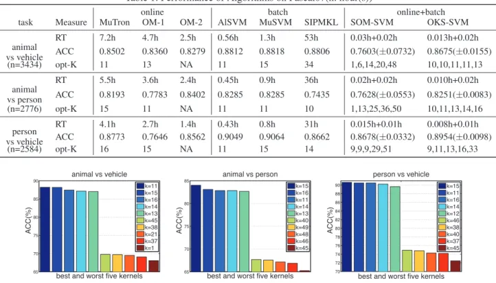
Table 1: Performance of Algorithms on Pascal07(h: hour(s))
online batch online+batch
task Measure MuTron OM-1 OM-2 AlSVM MuSVM SIPMKL SOM-SVM OKS-SVM RT 7.2h 4.7h 2.5h 0.56h 1.3h 53h 0.03h+0.02h 0.013h+0.02h animal vs vehicle ACC 0.8502 0.8360 0.8279 0.8812 0.8818 0.8806 0.7603(±0.0732) 0.8675(±0.0155) (n=3434) opt-K 11 13 NA 11 15 34 1,6,14,20,48 10,10,11,11,13 RT 5.5h 3.6h 2.4h 0.45h 0.9h 36h 0.02h+0.02h 0.010h+0.02h animal vs person ACC 0.8193 0.7783 0.8402 0.8285 0.8285 0.7435 0.7628(±0.0553) 0.8251(±0.0083) (n=2776) opt-K 15 11 NA 11 11 10 1,13,25,36,50 10,11,13,14,16 RT 4.1h 2.7h 1.4h 0.43h 0.8h 31h 0.015h+0.01h 0.008h+0.01h person vs vehicle ACC 0.8773 0.7646 0.8562 0.9049 0.9064 0.8662 0.8678(±0.0332) 0.8954(±0.0098) (n=2584) opt-K 16 15 NA 11 15 14 9,9,9,29,51 9,11,13,16,33
Figure 1: Accuracy of the best and the worst 5 kernels on the testing data of Pascal07 (Good kernels 9∼12 and 13∼16 are the 4 types of kernels defined on bag-of-words feature quantized from dense sift features at two layouts, respectively. Bad kernels 45∼48 are the 4 types of kernels defined on color histogram in LAB representation. Note that the best kernel11or15 is chi-square kernel.)
We report the results on the two data sets of different al-gorithms in Table 1, and 2, respectively, whereSOM-SVM andOKS-SVM refer to the approaches by running SOM and OKS first to select the best kernel and then running SVM with the selected kernel, respectively. We report three measures evaluated on different algorithms, i.e. the running time (RT)4, the accuracy on testing data (ACC) of the
re-turned kernel classifier5, and the returned optimal kernel id
(opt-K)6. Since SOM and OKS are stochastic algorithms, we
therefore run both algorithms with 5 different random seed-ings, and report the selected best kernel in each trial and the averaged ACC over the 5 random trials. Note that the run-ning time of SOM/OKS-SVM includes the runrun-ning time of SOM/OKS for selecting one kernel plus the running time of LibSVM for training a kernel classifier using the selected kernel. We did not report the results using the corresponding kernel classifier for the selected kernel by OKS, since we are
4
The running time includes the cross validation time for tun-ing the parameters, and the preprocesstun-ing time for computtun-ing the kernel matrices for MuSVM, AlSVM.
5
For MuTron, AlSVM, and MuSVM, the returned kernel clas-sifier is the selected best kernel clasclas-sifier, for OM-1, OM-2 and SIPMKL, the returned classifier is the combined kernel classifier.
6
The optimal kernels for OM-1 and SIPMKL shown in the Ta-bles are the ones that have the largest weight. OM-2 does not output any weight vector corresponding to kernels.
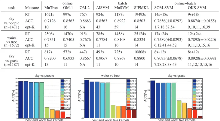
using OKS for selecting a good kernel. It is worth noting that by running OKS followed by Perceptron on the selected ker-nel we are able to obtain a good performance, which might be useful when training data is too huge to run batch kernel SVM. We also plot in Figure 1, 2 the accuracy of the best and the worst 5 kernel classifiers, which are trained by LibSVM and selected based on their performance on the testing data, which can be seen as the groundtruth to tell the performance of the best and the worst 5 kernels.
From these results, we can see that OKS can quickly iden-tify a good kernel, and the performance of OKS-SVM is comparable to MuSVM and MKL. Compared to SOM, the proposed OKS can select better kernels, which verifies the important extensions we made to SOM for online kernel se-lection.
Conclusions
In this paper, we propose online kernel selection algorithms. The empirical studies on image classification demonstrate the effectiveness of the proposed algorithms. In the future, we plan to extend the work in two dimensions: in algorith-mic dimension, we plan to derive algorithms that have high probability bounds in online setting, and in empirical dimen-sion, we plan to evaluate the online kernel selection algo-rithms on more prediction tasks and data sets.
Table 2: Performance of Algorithms on Corel5k(s: second(s))
online batch online+batch
task Measure MuTron OM-1 OM-2 AlSVM MuSVM SIPMKL SOM-SVM OKS-SVM RT 1621s 997s 767s 924s 1187s 19493s 14s+18s 9s+18s sky vs people ACC 0.7126 0.8563 0.8683 0.8563 0.8922 0.8503 0.7856(±0.0292) 0.8874(±0.0155) (n=1471) opt-K 10 16 NA 43 59 14 1,7,18,37,54 9,10,11,16,39 RT 2506s 1470s 915s 785s 1458s 25124s 17s+24s 12s+24s water vs tree ACC 0.7351 0.7405 0.7676 0.7784 0.8108 0.8324 0.7589(±0.0293) 0.7892(±0.0220) (n=1572) opt-K 15 15 NA 11 16 14 6,12,41,44,52 9,11,13,15,16 RT 817s 572s 447s 493s 725s 10808s 8s+12s 8s+12s sky vs grass ACC 0.8200 0.6933 0.8667 0.9067 0.8867 0.8800 0.8093(±0.0678) 0.8920(±0.0098) (n=1187) opt-K 13 11 NA 11 10 14 7,28,28,38,43 11,12,13,15,16
Figure 2: Accuracy of the best and the worst 5 kernels on the testing data of Corel5k (Bad kernels 21∼24 and 25∼28 are the 4 types of kernels defined on bag-of-words feature quantized from Hue descriptor extracted for Harris-Laplacian interest points at two layouts. Bad kernels 1∼4 are the 4 types of kernels defined on bag-of-words feature quantized from Hue descriptor extracted densely. )
Acknowledgments
This work was supported in part by National Science Foun-dation (IIS-0643494) and Office of Naval Research (ONR N00014-09-1-0663).
Appendix
Proof Sketch of Theorem 1
Let us introduce the notationsmti = I(it = i)andme
t
i =
mti/pti. It is easy to see thatEt[mti] = p t
iandEt[me
t i] = 1,
whereEtis taken expectation on random variablesit
con-ditioned on all previous random variables. Following the standard analysis of exponential weighted average algo-rithm (e.g. (Auer et al. 2003)), we first boundPT
t=1ln
Wt+1 Wt
from below and above.
T X t=1 lnWt+1 Wt ≥ −η T X t=1 e mti`(fi(xt), yt)−lnm T X t=1 lnWt+1 Wt ≤ −η T X t=1 m X i=1 qtimeti`(fit(xt), yt) +1 2η 2 T X t=1 m X i=1 qit(me t i`(f t i(xt), yt))2
Combing the lower bound and upper bound we have
T X t=1 m X i=1 qitmeti`(fit(xt), yt)≤ T X t=1 e mti`(fit(xt), yt) +1 2η T X t=1 m X i=1 qit mti (pt i)2 L2+lnm η
where we use upper bound|`(fit(xt), yt)| ≤Lto bound the
second order term `2(ft
i(xt), yt). Then we bound the first
order term`(fit(xt), yt)by`(f(xt), yt),∀f ∈ Hκi, i∈[m]
using the standard analysis of the gradient descent algorithm (e.g. (Nesterov 2004)), e mti(`(fit(xt), yt)−`(f(xt), yt)) ≤ hfit−f,meti∇`(fit(xt), yt)κi(xt,·)i ≤ 1 2λ kfit−fk2− kfit+1−fk2+m t i∇`2(fit(xt), yt)λ2 (pt i)2 ≤ 1 2λ kfit−fk2− kft+1 i −fk 2+mtiG2λ2 (pt i)2
By combining the above inequalities, taking expectation over randomness, and using simple algebra we can prove the theorem.
References
Abernethy, J.; Agarwal, A.; Bartlett, P. L.; and Rakhlin, A. 2009. A stochastic view of optimal regret through minimax duality. InCOLT.
Agarwal, A.; Duchi, J. C.; Bartlett, P. L.; and Levrard, C. 2011. Oracle inequalities for computationally budgeted model selection. InCOLT.
Akaike, H. 1974. A new look at the statistical model identification. Automatic Control, IEEE Transactions on
19(6):716–723.
Auer, P.; Cesa-Bianchi, N.; Freund, Y.; and Schapire, R. E. 2003. The nonstochastic multiarmed bandit problem. SIAM J. Comput.32:48–77.
Cesa-Bianchi, N., and Lugosi, G. 2006. Prediction, Learn-ing, and Games. New York, NY, USA: Cambridge Univer-sity Press.
Cortes, C.; Mohri, M.; and Rostamizadeh, A. 2010. Two-stage learning kernel algorithms. InICML, 239–246. Crammer, K.; Dekel, O.; Keshet, J.; Shalev-Shwartz, S.; and Singer, Y. 2006. Online passive-aggressive algorithms. J. Mach. Learn. Res.7:551–585.
Dekel, O.; Shalev-Shwartz, S.; and Singer, Y. 2005. The forgetron: A kernel-based perceptron on a fixed budget. In
NIPS.
Freund, Y., and Schapire, R. E. 1997. A decision-theoretic generalization of on-line learning and an application to boosting. J. Comput. Syst. Sci.55:119–139.
Guillaumin, M.; Mensink, T.; Verbeek, J. J.; and Schmid, C. 2009. Tagprop: Discriminative metric learning in nearest neighbor models for image auto-annotation. InICCV, 309– 316.
Guillaumin, M.; Verbeek, J. J.; and Schmid, C. 2010. Multi-modal semi-supervised learning for image classification. In
CVPR, 902–909.
Jebara, T.; Kondor, R.; and Howard, A. 2004. Probability product kernels. J. Mach. Learn. Res.819–844.
Jin, R.; Hoi, S. C. H.; and Yang, T. 2010. Online multiple kernel learning: Algorithms and mistake bounds. In ALT, 390–404.
Lampert, C. H. 2009. Kernel methods in computer vision.
Found. Trends. Comput. Graph. Vis.4:193–285.
Lanckriet, G.; Cristianini, N.; Bartlett, P.; and Ghaoui, L. E. 2004. Learning the kernel matrix with semidefinite pro-gramming. JMLR5:27–72.
Mallows, C. L. 1973. Some comments on cp.Technometrics
15:661–675.
Nesterov, Y. 2004. Introductory Lectures on Convex Opti-mization: A Basic Course (Applied Optimization). Springer Netherlands, 1 edition.
Orabona, F.; Luo, J.; and Caputo, B. 2010. Online-batch strongly convex multi kernel learning. InProceedings of the IEEE Conference on Computer Vision and Pattern Recogni-tion.
Rakotomamonjy, A.; Bach, F. R.; Canu, S.; and Grandvalet, Y. 2008. SimpleMKL. JMLR9:2491–2521.
Rosenblatt, F. 1958. The perceptron: A probabilistic model for information storage and organization in the brain. Psy-chological Review65(6):386–408.
Sch¨olkopf, B., and Smola, A. J. 2001. Learning with Ker-nels: Support Vector Machines, Regularization, Optimiza-tion, and Beyond. Cambridge, MA, USA: MIT Press. Sch¨olkopf, B.; Guyon, I.; and Weston, J. 2000. Statistical learning and kernel methods in bioinformatics. Technical report.
Schwarz, G. 1978. Estimating the dimension of a model.
The Annals of Statistics6(2):461–464.
Shwartz, S. S.; Singer, Y.; and Srebro, N. 2007. Pegasos: Primal estimated sub-GrAdient SOlver for SVM. In Pro-ceedings of the 24th international conference on Machine learning, 807–814.
Xu, Z.; Jin, R.; King, I.; and Lyu, M. R. 2008. An extended level method for efficient multiple kernel learning. InNIPS, 1825–1832.
Zhang, J.; Marszalek, M.; Lazebnik, S.; and Schmid, C. 2007. Local features and kernels for classification of texture and object categories: A comprehensive study.International Journal of Computer Vision213–238.