Diffusion Adaptation Strategies for Distributed
Optimization and Learning over Networks
Jianshu Chen, Student Member, IEEE, and Ali H. Sayed, Fellow, IEEE
Abstract
We propose an adaptive diffusion mechanism to optimize a global cost function in a distributed manner over a network of nodes. The cost function is assumed to consist of a collection of individual components. Diffusion adaptation allows the nodes to cooperate and diffuse information in real-time; it also helps alleviate the effects of stochastic gradient noise and measurement noise through a continu-ous learning process. We analyze the mean-square-error performance of the algorithm in some detail, including its transient and steady-state behavior. We also apply the diffusion algorithm to two problems: distributed estimation with sparse parameters and distributed localization. Compared to well-studied incremental methods, diffusion methods do not require the use of a cyclic path over the nodes and are robust to node and link failure. Diffusion methods also endow networks with adaptation abilities that enable the individual nodes to continue learning even when the cost function changes with time. Examples involving such dynamic cost functions with moving targets are common in the context of biological networks.
Index Terms
Distributed optimization, diffusion adaptation, incremental techniques, learning, energy conservation, biological networks, mean-square performance, convergence, stability.
I. INTRODUCTION
We consider the problem of optimizing a global cost function in a distributed manner. The cost function is assumed to consist of the sum of individual components, and spatially distributed nodes are used to
Manuscript received October 30, 2011; revised March 15, 2012. This work was supported in part by NSF grants CCF-1011918 and CCF-0942936. Preliminary results related to this work are reported in the conference presentations [1] and [2].
The authors are with Department of Electrical Engineering, University of California, Los Angeles, CA 90095. Email:{jshchen,
seek the common minimizer (or maximizer) through local interactions. Such problems abound in the context of biological networks, where agents collaborate with each other via local interactions for a common objective, such as locating food sources or evading predators [3]. Similar problems are common in distributed resource allocation applications and in online machine learning procedures. In the latter case, data that are generated by the same underlying distribution are processed in a distributed manner over a network of learners in order to recover the model parameters (e.g., [4], [5]).
There are already a few of useful techniques for the solution of optimization problems in a distributed manner [6]–[24]. Most notable among these methods is the incremental approach [6]–[9] and the con-sensus approach [10]–[23]. In the incremental approach, a cyclic path is defined over the nodes and data are processed in a cyclic manner through the network until optimization is achieved. However, determining a cyclic path that covers all nodes is known to be an NP-hard problem [25] and, in addition, cyclic trajectories are prone to link and node failures. When any of the edges along the path fails, the sharing of data through the cyclic trajectory is interrupted and the algorithm stops performing. In the consensus approach, vanishing step-sizes are used to ensure that nodes reach consensus and converge to the same optimizer in steady-state. However, in time-varying environments, diminishing step-sizes prevent the network from continuous learning and optimization; when the step-sizes die out, the network stops learning. In earlier publications [26]–[35], and motivated by our work on adaptation and learning over networks, we introduced the concept of diffusion adaptation and showed how this technique can be used to solve global minimum mean-square-error estimation problems efficiently both in real-time and
in a distributed manner. In the diffusion approach, information is processed locally and simultaneously
at all nodes and the processed data are diffused through a real-time sharing mechanism that ripples through the network continuously. Diffusion adaptation was applied to model complex patterns of behavior encountered in biological networks, such as bird flight formations [36] and fish schooling [3]. Diffusion adaptation was also applied to solve dynamic resource allocation problems in cognitive radios [37], to perform robust system identification [38], and to implement distributed online learning in pattern recognition applications [5].
This paper generalizes the diffusive learning process and applies it to the distributed optimization of a wide class of cost functions. The diffusion approach will be shown to alleviate the effect of gradient noise on convergence. Most other studies on distributed optimization tend to focus on the almost-sure convergence of the algorithms under diminishing step-size conditions [6], [7], [39]–[43], or on convergence under deterministic conditions on the data [6]–[8], [15]. In this article we instead examine the distributed algorithms from a mean-square-error perspective at constant step-sizes. This is because
constant step-sizes are necessary for continuous adaptation, learning, and tracking, which in turn enable the resulting algorithms to perform well even under data that exhibit statistical variations, measurement noise, and gradient noise.
This paper is organized as follows. In Sec. II, we introduce the global cost function and approximate it by a distributed optimization problem through the use of a second-order Taylor series expansion. In Sec. III, we show that optimizing the localized alternative cost at each nodekleads naturally to diffusion adaptation strategies. In Sec. IV, we analyze the mean-square performance of the diffusion algorithms under statistical perturbations when stochastic gradients are used. In Sec. V, we apply the diffusion algorithms to two application problems: sparse distributed estimation and distributed localization. Finally, in Sec. VI, we conclude the paper.
Notation. Throughout the paper, all vectors are column vectors except for the regressors {uk,i}, which are taken to be row vectors for simplicity of notation. We use boldface letters to denote random quantities (such asuk,i) and regular font letters to denote their realizations or deterministic variables (such asuk,i). We write E to denote the expectation operator. We use diag{x1, . . . , xN} to denote a diagonal matrix consisting of diagonal entries x1, . . . , xN, and use col{x1, . . . , xN} to denote a column vector formed by stacking x1, . . . , xN on top of each other. For symmetric matrices X and Y, the notation X ≤ Y denotes Y −X≥0, namely, that the matrix difference Y −X is positive semi-definite.
II. PROBLEMFORMULATION
The objective is to determine, in a collaborative and distributed manner, the M×1column vector wo that minimizes a global cost of the form:
Jglob(w) = N
X
l=1
Jl(w) (1)
whereJl(w),l= 1,2, . . . , N, are individual real-valued functions, defined overw∈RM and assumed to be differentiable and strictly convex. Then, Jglob(w) in (1) is also strictly convex so that the minimizer
wo is unique [44]. In this article we study the important case where the component functions{Jl(w)}are minimized at thesamewo. This case is common in practice; situations abound where nodes in a network need to work cooperatively to attain a common objective (such as tracking a target, locating the source of chemical leak, estimating a physical model, or identifying a statistical distribution). This scenario is also frequent in the context of biological networks. For example, during the foraging behavior of an animal group, each agent in the group is interested in determining the same vectorwo that corresponds
in online distributed machine learning problems, where data samples are often generated from the same underlying distribution and they are processed in a distributed manner by different nodes (e.g., [4], [5]). The case where the{Jl(w)}have different individual minimizers is studied in [45]; this situation is more challenging to study. Nevertheless, it is shown in [45] that the same diffusion strategies (18)–(19) of this paper are still applicable and nodes would converge instead to a Pareto-optimal solution.
Our strategy to optimize the global cost Jglob(w) in a distributed manner is based on three steps. First, using a second-order Taylor series expansion, we argue that Jglob(w) can be approximated by an alternative localized cost that is amenable to distributed optimization — see (11). Second, each individual node optimizes this alternative cost via a steepest-descent procedure that relies solely on interactions within the neighborhood of the node. Finally, the local estimates for wo are spatially combined by each node and the procedure repeats itself in real-time.
To motivate the approach, we start by introducing a set of nonnegative coefficients {cl,k}that satisfy: N
X
k=1
cl,k = 1, cl,k = 0 if l /∈ Nk, l= 1,2, . . . , N (2)
whereNk denotes the neighborhood of nodek(including nodekitself); the neighbors of nodekconsist of all nodes with which node k can share information. Each cl,k represents a weight value that node
k assigns to information arriving from its neighbor l. Condition (2) states that the sum of all weights leaving each nodel should be one. Using the coefficients {cl,k}, we can express Jglob(w) from (1) as
Jglob(w) =Jkloc(w) + N X l6=k Jlloc(w) (3) where Jloc k (w), X l∈Nk cl,kJl(w) (4)
In other words, for each nodek, we are introducing a new local cost function,Jloc
k (w), which corresponds to a weighted combination of the costs of its neighbors. Since the {cl,k} are all nonnegative and each
Jl(w) is convex, thenJkloc(w) is also a convex function (actually, the Jkloc(w) will be guaranteed to be strongly convex in our treatment in view of Assumption 1 further ahead).
Now, each Jloc
l (w) in the second term of (3) can be approximated via a second-order Taylor series expansion as:
Jlloc(w)≈Jlloc(wo) +kw−wok2Γ
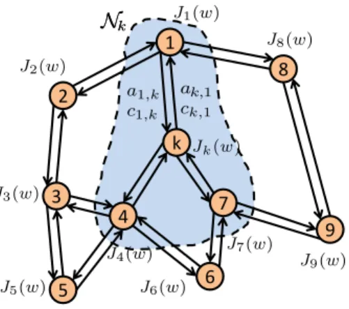
1 2 4 8 7 k 5 9 3 6 Nk Nk ak;1 ck;1 Jk(w) J1(w) J2(w) J3(w) J5(w) J6(w) J4(w) J7(w) J9(w) J8(w) a1;k c1;k
Fig. 1. A network withN nodes; a cost functionJk(w)is associated with each node k. The set of neighbors of nodek is denoted byNk; this set consists of all nodes with which nodek can share information.
where Γl=12∇2
wJlloc(wo) is the (scaled) Hessian matrix relative to w and evaluated at w=wo, and the notation kak2
Σ denotes aTΣa for any weighting matrix Σ. The analysis in the subsequent sections will show that the second-order approximation (5) is sufficient to ensure mean-square convergence of the resulting diffusion algorithm. Now, substituting (5) into the right-hand side of (3) gives:
Jglob(w)≈Jkloc(w)+X l6=k
kw−wok2Γl+X l6=k
Jlloc(wo) (6)
The last term in the above expression does not depend on the unknown w. Therefore, we can ignore it so that optimizing Jglob(w) is approximately equivalent to optimizing the following alternative cost:
Jglob0 (w),Jloc k (w) + X l6=k kw−wok2 Γl (7)
III. ITERATIVEDIFFUSIONSOLUTION
Expression (7) relates the original global cost (1) to the newly-defined local cost function Jloc k (w). The relation is through the second term on the right-hand side of (7), which corresponds to a sum of quadratic terms involving the minimizerwo. Obviously,wois not available at nodeksince the nodes wish to estimatewo. Likewise, not all Hessian matricesΓlare available to nodek. Nevertheless, expression (7) suggests a useful approximation that leads to a powerful distributed solution, as we proceed to explain.
Our first step is to replace the global cost Jglob0
(w) by a reasonable localized approximation for it at every node k. Thus, initially we limit the summation on the right-hand side of (7) to the neighbors of node kand introduce the cost function:
Jkglob0(w),Jloc k (w) +
X
kw−wok2
Compared with (7), the last term in (8) involves only quantities that are available in the neighborhood of node k. The argument involving steps (5)–(8) therefore shows us one way by which we can adjust the earlier local cost function Jloc
k (w) defined in (4) by adding to it the last term that appears in (8). Doing so, we end up replacingJloc
k (w) byJ glob0
k (w), and this new localized cost function preserves the second term in (3) up to a second-order approximation. This correction will help lead to a diffusion step (see (14)–(15)).
Now, observe that the cost in (8) includes the quantities{Γl}, which belong to the neighbors of nodek. These quantities may or may not be available. If they are known, then we can proceed with (8) and rely on the use of the Hessian matrices Γl in the subsequent development. Nevertheless, the more interesting situation in practice is when these Hessian matrices are not known beforehand (especially since they depend on the unknownwo). For this reason, in this article, we approximate eachΓ
l in (8) by a multiple of the identity matrix, say,
Γl≈bl,kIM (9)
for some nonnegative coefficients {bl,k}; observe that we are allowing the coefficient bl,k to vary with the node index k. Such approximations are common in stochastic approximation theory and help reduce the complexity of the resulting algorithms — see [44, pp.20–28] and [46, pp.142–147]. Approximation (9) is reasonable since, in view of the Rayleigh-Ritz characterization of eigenvalues [47], we can always bound the weighted squared norm kw−wok2
Γl by the unweighted squared norm as follows
λmin(Γl)· kw−wok2 ≤ kw−wok2Γl ≤λmax(Γl)· kw−w ok2 Thus, we replace (8) by Jkglob00(w),Jkloc(w) + X l∈Nk\{k} bl,kkw−wok2 (10)
As the derivation will show, we do not need to worry at this stage about how the scalars {bl,k} are selected; they will be embedded into other combination weights that the designer selects. If we replace
Jloc
k (w) by its definition (4), we can rewrite (10) as
Jkglob00(w) = X l∈Nk cl,kJl(w) + X l∈Nk\{k} bl,kkw−wok2 (11)
Observe that cost (11) is different for different nodes; this is because the choices of the weighting scalars {cl,k, bl,k} vary across nodes k; moreover, the neighborhoods vary with k. Nevertheless, these localized cost functions now constitute the important starting point for the development of diffusion strategies for the online and distributed optimization of (1).
Each nodekcan apply a steepest-descent iteration to minimizeJkglob00(w)by moving along the negative direction of the gradient (column) vector of the cost function, namely,
wk,i=wk,i−1−µk X l∈Nk cl,k∇wJl(wk,i−1) −µk X l∈Nk\{k} 2bl,k(wk,i−1−wo), i≥0 (12) where wk,i denotes the estimate for wo at node k at time i, and µk denotes a small constant positive step-size parameter. While vanishing step-sizes, such asµk(i) = 1/i, can be used in (12), we consider in this paper the case of constant step-sizes. This is because we are interested in distributed strategies that are able to continue adapting and learning. An important question to address therefore is how close each of the wk,i gets to the optimal solution wo; we answer this question later in the paper by means of a error convergence analysis (see expression (88)). It will be seen then that the mean-square-error (MSE) of the algorithm will be of the order of the step-size; hence, sufficiently small step-sizes will lead to sufficiently small MSEs.
Expression (12) adds two correction terms to the previous estimate, wk,i−1, in order to update it to
wk,i. The correction terms can be added one at a time in a succession of two steps, for example, as:
ψk,i=wk,i−1−µk X l∈Nk cl,k∇wJl(wk,i−1) (13) wk,i=ψk,i−µk X l∈Nk\{k} 2bl,k(wk,i−1−wo) (14) Step (13) updateswk,i−1 to an intermediate value ψk,i by using a combination of local gradient vectors. Step (14) further updates ψk,i to wk,i by using a combination of local estimates. However, two issues arise while examining (14):
(a) First, iteration (14) requires knowledge of the optimizerwo. However, all nodes are running similar updates to estimate thewo. By the time node k wishes to apply (14), each of its neighbors would have performed its own update similar to (13) and would have available their intermediate estimates, {ψl,i}. Therefore, we replacewoin (14) byψl,i. This step helps diffuse information over the network and brings into nodekinformation that exists beyond its immediate neighborhood; this is because each ψl,i is influenced by data from the neighbors of node l. We observe that this diffusive term arises from the quadratic approximation (5) we have made to the second term in (3).
(b) Second, the intermediate value ψk,i in (13) is generally a better estimate for wo than wk,i−1 since it is obtained by incorporating information from the neighbors through (13). Therefore, we
further replace wk,i−1 in (14) byψk,i. This step is reminiscent of incremental-type approaches to optimization, which have been widely studied in the literature [6]–[9].
Performing the substitutions described in items (a) and (b) into (14), we obtain:
wk,i=ψk,i−µk
X
l∈Nk\{k}
2bl,k(ψk,i−ψl,i) (15)
Now introduce the coefficients
al,k ,2µkbl,k (l6=k), ak,k ,1−µk
X
l∈Nk\{k}
2bl,k (16)
Note that the {al,k} are nonnegative forl 6=k and ak,k ≥0 for sufficiently small step-sizes. Moreover, the coefficients {al,k} satisfy
N
X
l=1
al,k = 1, al,k = 0 if l /∈ Nk (17)
Using (16) in (15), we arrive at the following Adapt-then-Combine (ATC) diffusion strategy (whose structure is the same as the ATC algorithm originally proposed in [29]–[31] for mean-square-error estimation): ψk,i=wk,i−1−µk X l∈Nk cl,k∇wJl(wk,i−1) wk,i= X l∈Nk al,kψl,i (18)
To run algorithm (18), we only need to select combination coefficients{al,k, cl,k}satisfying (2) and (17), respectively; there is no need to worry about the intermediate coefficients {bl,k} any more, since they have been blended into the {al,k}. The ATC algorithm (18) involves two steps. In the first step, node k receives gradient vector information from its neighbors and uses it to update its estimate wk,i−1 to an intermediate valueψk,i. All other nodes in the network are performing a similar step and generating their intermediate estimateψl,i. In the second step, nodekaggregates the estimates{ψl,i} of its neighbors and generateswk,i. Again, all other nodes are performing a similar step. Similarly, if we reverse the order of steps (13) and (14) to implement (12), we can motivate the following alternative Combine-then-Adapt (CTA) diffusion strategy (whose structure is similar to the CTA algorithm originally proposed in [26]–[32] for mean-square-error estimation):
ψk,i−1= X l∈Nk al,kwl,i−1 wk,i=ψk,i−1−µk X l∈Nk cl,k∇wJl(ψk,i−1) (19)
Adaptive diffusion strategies of the above ATC and CTA types were first proposed and extended in [26]– [34] for the solution of distributed mean-square-error, least-squares, and state-space estimation problems over networks. The special form of ATC strategy (18) for minimum-mean-square-error estimation is listed further ahead as Eq. (57) in Example 3; the same strategy as (57) also appeared in [48] albeit with a vanishing step-size sequence to ensure convergence towards consensus. A special case of the diffusion strategy (19) (corresponding to choosing cl,k = 0 for l6=k and ck,k = 1, i.e., without sharing gradient information) was used in the works [39], [40], [43] to solve distributed optimization problems that require all nodes to reach agreement about wo by relying on step-sizes that decay to zero with time. Diffusion recursions of the forms (18) and (19) are more general than these earlier investigations in a couple of respects. First, they do not only diffuse the local estimates, but they can also diffuse the local gradient vectors. In other words, two sets of combination coefficients{al,k, cl,k}are used. Second, the combination weights{al,k} are not required to be doubly stochastic (which would require both the rows and columns of the weighting matrix A= [al,k] to add up to one; as seen from (17), we only require the entries on the columns ofAto add up to one). Finally, and most importantly, the step-size parameters {µk} in (18) and (19) are not required to depend on the time indexiand are not required to vanish asi→ ∞. Instead, they can assume constant values, which is critical to endow the network with continuousadaptation and learning abilities (otherwise, when step-sizes die out, the network stops learning). Constant step-sizes also endow networks with tracking abilities, in which case the algorithms can track time changes in the optimal wo.
Constant step-sizes will be shown further ahead to be sufficient to guarantee agreement among the nodes when there is no noise in the data. However, when measurement noise and gradient noise are present, using constant step-sizes does notforce the nodes to attain agreement aboutwo (i.e., to converge to the same wo). Instead, the nodes will be shown to tend to individual estimates forwo that are within a small mean-square-error (MSE) bound from the optimal solution; the bound will be proportional to the step-size so that sufficiently small step-sizes lead to small MSE values. Multi-agent systems in nature behave in this manner; they do not require exact agreement among their agents but allow for fluctuations due to individual noise levels (see [3], [36]). Giving individual nodes this flexibility, rather than forcing them to operate in agreement with the remaining nodes, ends up leading to nodes with enhanced learning abilities.
Before proceeding to a detailed analysis of the performance of the diffusion algorithms (18)–(19), we note that these strategies differ in important ways from traditional consensus-based distributed solutions,
which are of the following form [10], [14], [15], [18]:
wk,i=
X
l∈Nk
al,kwk,i−1−µk(i)· ∇wJl(wk,i−1) (20) usually with a time-variant step-size sequence, µk(i), that decays to zero. For example, if we set C , [cl,k] = I in the CTA algorithm (19) and substitute the combination step into the adaptation step, we obtain: wk,i= X l∈Nk al,kwk,i−1−µk∇wJl X l∈Nk al,kwk,i−1 ! (21)
Thus, note that the gradient vector in (21) is evaluated at ψk,i−1, while in (20) it is evaluated at wk,i−1. Sinceψk,i−1 already incorporates information from neighbors, we would expect the diffusion algorithm to perform better. Actually, it is shown in [49] that, for mean-square-error estimation problems, diffusion strategies achieve higher convergence rate and lower mean-square-error than consensus strategies due to these differences in the dynamics of the algorithms.
IV. MEAN-SQUAREPERFORMANCEANALYSIS
The diffusion algorithms (18) and (19) depend on sharing local gradient vectors ∇wJl(·). In many cases of practical relevance, the exact gradient vectors are not available and approximations are instead used. We model the inaccuracy in the gradient vectors as some random additive noise component, say, of the form:
b
∇wJl(w) =∇wJl(w) +vl,i(w) (22)
where vl,i(·) denotes the perturbation and is often referred to as gradient noise. Note that we are using a boldface symbolv to refer to the gradient noise since it is generally stochastic in nature.
Example 1. Assume the individual cost Jl(w) at node l can be expressed as the expected value of a certain loss function Ql(·,·), i.e., Jl(w) = E{Ql(w,xl,i)}, where the expectation is with respect to the
randomness in the data samples{xl,i}that are collected at node lat time i. Then, if we replace the true gradient ∇wJl(w) with its stochastic gradient approximation ∇bwJl(w) = ∇wQl(w,xl,i), we find that
the gradient noise in this case can be expressed as
Using the perturbed gradient vectors (22), the diffusion algorithms (18)–(19) become the following: (ATC) ψk,i=wk,i−1−µk X l∈Nk cl,k∇bwJl(wk,i−1) wk,i= X l∈Nk al,kψl,i (24) (CTA) ψk,i−1 = X l∈Nk al,kwl,i−1 wk,i=ψk,i−1−µk X l∈Nk cl,k∇bwJl(ψk,i−1) (25)
Observe that, starting with (24)–(25), we will be using boldface letters to refer to the various estimate quantities in order to highlight the fact that they are also stochastic in nature due to the presence of the gradient noise.
Given the above algorithms, it is necessary to examine their performance in light of the approximation steps (6)–(15) that were employed to arrive at them, and in light of the gradient noise (22) that seeps into the recursions. A convenient framework to carry out this analysis is mean-square analysis. In this framework, we assess how close the individual estimateswk,iget to the minimizerwoin the mean-square-error (MSE) sense. In practice, it is not necessary to force the individual agents to reach agreement and to converge to the same wo using diminishing step-sizes. It is sufficient for the nodes to converge within acceptable MSE bounds from wo. This flexibility is beneficial and is common in biological networks; it allows nodes to learn and adapt in time-varying environments without the forced requirement of having to agree with neighbors.
The main results that we derive in this section are summarized as follows. First, we derive conditions on the constant step-sizes to ensure boundedness and convergence of the mean-square-error for sufficiently small step-sizes — see (80) and (106) further ahead. Second, despite the fact that nodes influence each other’s behavior, we are able to quantify the performance of every node in the network and to derive closed-form expressions for the mean-square performance at small step-sizes — see (106)–(108). Finally, as a special case, we are able to show that constant step-sizes can still ensure that the estimates across all nodes converge to the optimalwo and reach agreement in the absence of noise— see Theorem 2.
Motivated by [31], we address the mean-square-error performance of the adaptive ATC and CTA diffusion strategies (24)–(25) by treating them as special cases of a general diffusion structure of the
following form: φk,i−1= N X l=1 p1,l,kwl,i−1 (26) ψk,i=φk,i−1−µk N X l=1 sl,k h
∇wJl(φk,i−1) +vl,i(φk,i−1)
i (27) wk,i= N X l=1 p2,l,kψl,i (28)
The coefficients{p1,l,k},{sl,k}, and{p2,l,k}are nonnegative real coefficients corresponding to the{l, k }-th entries of }-three matrices P1, S, andP2, respectively. Different choices for{P1, P2, S} correspond to different cooperation modes. For example, the choice P1 = I, P2 = I and S = I corresponds to the non-cooperative case where nodes do not interact. On the other hand, the choiceP1 =I,P2 =A= [al,k] and S = C = [cl,k] corresponds to ATC [29]–[31], while the choice P1 = A, P2 = I and S = C corresponds to CTA [26]–[31]. We can also set S =I in ATC and CTA to derive simplified versions that have no gradient exchange [29]. Furthermore, if in CTA (P2=I), we enforceP1=Ato be doubly stochastic, set S = I, and use a time-decaying step-size parameter (µk(i) → 0), then we obtain the unconstrained version used by [39], [43]. The matrices {P1, P2, S} are required to satisfy:
P1T1=1, P2T1=1, S1=1 (29)
where the notation1 denotes a vector whose entries are all equal to one.
A. Error Recursions
We first derive the error recursions corresponding to the general diffusion formulation in (26)–(28). Introduce the error vectors:
˜
φk,i,wo−φk,i, ψ˜k,i,wo−ψk,i, w˜k,i,wo−wk,i (30)
Then, subtracting both sides of (26)–(28) from wo gives:
˜ φk,i−1= N X l=1 p1,l,kw˜l,i−1 (31) ˜ ψk,i= ˜φk,i−1+µk N X l=1 sl,k h
∇wJl(φk,i−1) +vl,i(φk,i−1)
i (32) ˜ wk,i= N X l=1 p2,l,kψ˜l,i (33)
Expression (32) still includes terms that depend on φk,i−1 and not on the error quantity, φ˜k,i−1. We can find a relation in terms of φ˜k,i−1 by calling upon the following result from [44, p.24] for any twice-differentiable function f(·): ∇f(y) =∇f(x) + Z 1 0 ∇2fx+t(y−x)dt (y−x) (34)
where∇2f(·) denotes the Hessian matrix off(·)and is symmetric. Now, since each component function
Jl(w) has a minimizer at wo, then, ∇wJl(wo) = 0 for l = 1,2, . . . , N. Applying (34) to Jl(w) using
x=wo andy =φ k,i−1, we get ∇wJl(φk,i−1) = ∇wJl(wo)− Z 1 0 ∇2wJl wo−tφ˜k,i−1 dt ˜ φk,i−1 ,−Hl,k,i−1φ˜k,i−1 (35) where we are introducing the symmetric random matrix
Hl,k,i−1 , Z 1 0 ∇2wJl wo−tφ˜k,i−1 dt (36)
Observe that one such matrix is associated with every edge linking two nodes(l, k); observe further that this matrix changes with time since it depends on the estimate at nodek. Substituting (35)–(36) into (32) leads to: ˜ ψk,i= " IM −µk N X l=1 sl,kHl,k,i−1 # ˜ φk,i−1 +µk N X l=1 sl,kvl,i(φk,i−1) (37) We introduce the network error vectors, which collect the error quantities across all nodes:
˜ φi , ˜ φ1,i .. . ˜ φN,i , ψ˜i , ˜ ψ1,i .. . ˜ ψN,i , w˜i , ˜ w1,i .. . ˜ wN,i (38)
and the following block matrices: P1 =P1⊗IM, P2 = P2⊗IM (39) S =S⊗IM, M = Ω⊗IM (40) Ω = diag{µ1, . . . , µN} (41) Di−1 = N X l=1 diagnsl,1Hl,1,i−1,· · ·, sl,NHl,N,i−1 o (42) gi = N X l=1
colnsl,1vl,i(φ1,i−1),· · · ,sl,Nvl,i(φN,i−1)
o
(43)
where the symbol ⊗denotes Kronecker products [50]. Then, recursions (31), (37) and (33) lead to:
˜
wi =P2T[IM N − MDi−1]P1Tw˜i−1+P2TMgi (44) To proceed with the analysis, we introduce the following assumption on the cost functions and gradient noise, followed by a lemma onHl,k,i−1.
Assumption 1(Bounded Hessian). Each component cost functionJl(w)has a bounded Hessian matrix, i.e., there exist nonnegative real numbersλl,min andλl,maxsuch that λl,min≤λl,max and that for allw:
λl,minIM ≤ ∇2wJl(w)≤λl,maxIM (45)
Furthermore, the {λl,min}Nl=1 satisfy N
X
l=1
sl,kλl,min>0, k= 1,2, . . . , N (46)
Condition (46) ensures that the local cost functions {Jloc
k (w)} defined earlier in (4) are strongly convex and, hence, have a unique minimizer at wo.
Assumption 2 (Gradient noise). There exist α≥0 andσ2
v ≥0 such that, for all w∈ Fi−1 and for all
i, l:
E{vl,i(w)| Fi−1}= 0 (47)
Ekvl,i(w)k2 ≤αEkwo−wk2+σv2 (48)
Lemma 1(Bound onHl,k,i−1). Under Assumption 1, the matrixHl,k,i−1defined in(36)is a
nonnegative-definite matrix that satisfies:
λl,minIM ≤Hl,k,i−1 ≤λl,maxIM (49) Proof: It suffices to prove that λl,min≤xTHl,k,i−1x≤λl,max for arbitrary M×1 unit Euclidean norm vectors x. By (36) and (45), we have
xTHl,k,i−1x= Z 1 0 xT∇2wJl wo−tφ˜k,i−1 x dt ≤ Z 1 0 λl,maxdt=λl,max In a similar way, we can verify that xTH
l,k,i−1x≥λl,min.
In distributed subgradient methods (e.g., [15], [39], [43]), the norms of the subgradients are usually required to be uniformly bounded. Such assumption is restrictive in the unconstrained optimization of differentiable functions. Assumption 1 is more relaxed in that it allows the gradient vector ∇wJl(w) to have unbounded norm (e.g., quadratic costs). Furthermore, condition (48) allows the variance of the gradient noise to grow no faster than Ekwo−wk2. This condition is also more general than the uniform
bounded assumption used in [39] (Assumptions 5.1 and 6.1), which requires instead:
Ekvl,i(w)k2≤σ2v, E
kvl,i(w)k2|Fi−1 ≤σv2 (50) Furthermore, condition (48) is similar to condition (4.3) in [51, p.635]:
Ekvl,i(w)k2|Fi−1 ≤α
h
k∇wJl(w)k2+ 1
i
(51)
which is a combination of the “relative random noise” and the “absolute random noise” conditions defined in [44, pp.100–102]. Indeed, we can derive (48) by substituting (35) into (51), taking expectation with respect to Fi−1, and then using (49).
Example 2. Such a mix of “relative random noise” and “absolute random noise” is of practical impor-tance. For instance, consider an example in which the loss function at node l is chosen to be of the following quadratic form:
Ql(w,{ul,i,dl(i)}) =|dl(i)−ul,iw|2
for some scalars {dl(i)} and1×M regression vectors {ul,i}. The corresponding cost function is then:
Assume further that the data {ul,i,dl(i)} satisfy the linear regression model
dl(i) =ul,iwo+zl(i) (53)
where the regressors {ul,i} are zero mean and independent over time with covariance matrix Ru,l =
E{uTl,iul,i}, and the noise sequence{zk(j)}is also zero mean, white, with varianceσz,k2 , and independent of the regressors {ul,i}for all l, k, i, j. Then, using (53) and (23), the gradient noise in this case can be expressed as:
vl,i(w) = 2(Ru,l−uTl,iul,i)(wo−w)−2uTl,izl(i) (54)
It can easily be verified that this noise satisfies both conditions stated in Assumption 2, namely, (47) and also:
Ekvl,i(w)k2
≤4EkRu,l−uTl,iul,ik2·Ekwo−wk2+4σz,l2 Tr(Ru,l) (55)
for allw∈ Fi−1. Note that both relative random noise and absolute random noise components appear in (55) and are necessary to model the statistical gradient perturbation even for quadratic costs. Such costs, and linear regression models of the form (53), arise frequently in the context of adaptive filters — see, e.g., [9], [26]–[33], [36], [46], [52]–[55].
Example 3. Quadratic costs of the form (52) are common in mean-square-error estimation for linear regression models of the type (53). If we use the instantaneous approximations as is common in the context of stochastic approximation and adaptive filtering [44], [46], [52], then the actual gradient∇wJl(w) can be approximated by
b
∇wJl(w) =∇wQl(w,{ul,i,dl(i)})
=−2uTl,i[dl(i)−ul,iw] (56)
Substituting into (24)–(25), and assumingC=I for illustration purposes only, we arrive at the following ATC and CTA diffusion strategies originally proposed and extended in [26]–[31] for the solution of distributed mean-square-error estimation problems:
(ATC)
ψk,i=wk,i−1+2µkuTk,i[dk(i)−uk,iwk,i−1]
wk,i=
X
l∈Nk
al,kψl,i
(CTA)
ψk,i−1=
X
l∈Nk
al,kwl,i−1
wk,i=ψk,i−1+2µkuTk,i[dk(i)−uk,iψk,i−1]
(58)
B. Variance Relations
The purpose of the mean-square analysis in the sequel is to answer two questions in the presence of gradient perturbations. First, how small the mean-square error, Ekw˜k,ik2, gets as i → ∞ for any of the nodes k. Second, how fast this error variance tends towards its steady-state value. The first question pertains to steady-state performance and the second question pertains to transient/convergence rate performance. Answering such questions for a distributed algorithm over a network is a challenging task largely because the nodes influence each other’s behavior: performance at one node diffuses through the network to the other nodes as a result of the topological constraints linking the nodes. The approach we take to examine the mean-square performance of the diffusion algorithms is by studying how the variance Ekw˜k,ik2, or a weighted version of it, evolves over time. As the derivation will show, the evolution of this variance satisfies a nonlinear relation. Under some reasonable assumptions on the noise profile, and the local cost functions, we will be able to bound these error variances as well as estimate their steady-state values for sufficiently small step-sizes. We will also derive closed-form expressions that characterize the network performance. The details are as follows.
Equating the squaredweighted Euclidean norm of both sides of (44), applying the expectation operator and using using (47), we can show that the following variance relation holds:
Ekw˜ik2Σ =E n kw˜i−1k2Σ0 o +EkP2TMgik2Σ Σ0 =P1[IM N−MDi−1]P2ΣP2T[IM N−MDi−1]P1T (59)
whereΣis a positive semi-definite weighting matrix that we are free to choose. The variance expression (59) shows how the quantity Ekw˜ik2Σ evolves with time. Observe, however, that the weighting matrix on w˜i−1 on the right-hand side of (59) is a different matrix, denoted by Σ0, and this matrix is actually random in nature (while Σ is deterministic). As such, result (59) is not truly a recursion. Nevertheless, it is possible, under a small step-size approximation, to rework variance relations such as (59) into a recursion by following certain steps that are characteristic of the energy conservation approach to mean-square analysis [46].
onφ˜k,i−1 as well, which in turn is a linear combination of the{w˜l,i−1}. Therefore, the main challenge to continue from (59) is that Σ0 depends onw˜i−1. For this reason, we cannot apply directly the traditional step of replacing Σ0 in the first equation of (59) by EΣ0 as is typically done in the study of stand-alone
adaptive filters to analyze their transient behavior [46, p.345]; in the case of conventional adaptive filters, the matrix Σ0 is independent of w˜i−1. To address this difficulty, we shall adjust the argument to rely on a set ofinequality recursions that will enable us to bound the steady-state mean-square-error at each node — see Theorem 1 further ahead.
The procedure is as follows. First, we note that kxk2 is a convex function of x, and that expressions (31) and (33) are convex combinations of{w˜l,i−1}and{ψ˜l,i}, respectively. Then, by Jensen’s inequality [56, p.77] and taking expectations, we obtain
Ekφ˜k,i−1k2≤ N X l=1 p1,l,kEkw˜l,i−1k2 (60) Ekw˜k,ik2≤ N X l=1 p2,l,kEkψ˜l,ik2 (61)
fork= 1, . . . , N. Next, we derive a variance relation for (37). Equating the squared Euclidean norms of both sides of (37), applying the expectation operator, and using (47) from Assumption 2, we get
Ekψ˜k,ik2=E n kφ˜k,i−1k2Σk,i−1 o +µ2kE N X l=1 sl,kvl,i(φk,i−1) 2 (62) where Σk,i−1 = " IM−µk N X l=1 sl,kHl,k,i−1 #2 (63)
We call upon the following two lemmas to bound (62).
Lemma 2 (Bound on Σk,i−1). The weighting matrix Σk,i−1 defined in (63) is a symmetric, positive
semi-definite matrix, and satisfies:
0≤Σk,i−1≤γk2IM (64) where γk ,max ( 1−µk N X l=1 sl,kλl,max , 1−µk N X l=1 sl,kλl,min ) (65)
Proof: By definition (63) and the fact that Hl,k,i−1 is symmetric — see definition (36), the matrix
IM−µkPNl=1sl,kHl,k,i−1is also symmetric. Hence, its square,Σk,i−1, is symmetric and also nonnegative-definite. To establish (64), we first use (49) to note that:
IM−µk N X l=1 sl,kHl,k,i−1≥ 1−µk N X l=1 sl,kλl,max ! IM (66) IM−µk N X l=1 sl,kHl,k,i−1≤ 1−µk N X l=1 sl,kλl,min ! IM (67)
The matrix IM −µkPlN=1sl,kHl,k,i−1 may not be positive semi-definite because we have not specified a range for µk yet; the expressions on the right-hand side of (66)–(67) may still be negative. However, inequalities (66)–(67) imply that the eigenvalues ofIM−µkPlN=1sl,kHl,k,i−1 are bounded as:
λ IM −µk N X l=1 sl,kHl,k,i−1 ! ≥1−µk N X l=1 sl,kλl,max (68) λ IM −µk N X l=1 sl,kHl,k,i−1 ! ≤1−µk N X l=1 sl,kλl,min (69)
By definition (63),Σk,i−1 is the square of the symmetric matrixIM−µk
PN
l=1sl,kHl,k,i−1, meaning that
λ(Σk,i−1) = " λ IM −µk N X l=1 sl,kHl,k,i−1 !#2 ≥0 (70)
Substituting (68)–(69) into (70) leads to
λ(Σk,i−1) ≤max ( 1−µk N X l=1 sl,kλl,max 2 , 1−µk N X l=1 sl,kλl,min 2) (71) which is equivalent to (64).
Lemma 3 (Bound on noise combination). The second term on the right-hand-side of (62) satisfies:
E N X l=1 sl,kvl,i(φk,i−1) 2 ≤ kSk21·hαEkφ˜k,i−1k2+σv2 i (72)
Proof: Applying Jensen’s inequality [56, p.77], it holds that E N X l=1 sl,kvl,i(φk,i−1) 2 = N X l=1 sl,k 2 ·E N X l=1 sl,k PN l=1sl,k vl,i(φk,i−1) 2 ≤ N X l=1 sl,k 2 · N X l=1 sl,k PN l=1sl,k Ekvl,i(φk,i−1)k2 = N X l=1 sl,k · N X l=1 sl,kEkvl,i(φk,i−1)k2 ≤ N X l=1 sl,k 2 ·hαEkφ˜k,i−1k2+σv2 i (73) ≤ kSk21·hαEkφ˜k,i−1k2+σ2v i (74)
where inequality (73) follows by substituting (48), and (74) is obtained using the fact that kSk1 is the maximum absolute column sum and that the entries {sl,k}are nonnegative.
Substituting (64) and (72) into (62), we obtain:
Ekψ˜k,ik2 ≤(γk2+µ2kαkSk21)·Ekφ˜k,i−1k2+µ2kkSk21 σv2 (75) for k = 1, . . . , N. Finally, introduce the following network mean-square-error vectors (compare with (38)): Xi = Ekφ˜1,ik2 .. . Ekφ˜N,ik2 , Yi= Ekψ˜1,ik2 .. . Ekψ˜N,ik2 , Wi = Ekw˜1,ik2 .. . Ekw˜N,ik2
and the matrix
Γ = diag
γ21+µ21αkSk21, . . . , γN2 +µ2NαkSk21 (76)
Then, (60)–(61) and (75) can be written as
Xi−1 P1TWi−1 Yi ΓXi−1+σ2vkSk21Ω21 WiP2TYi (77)
where the notation x y denotes that the components of vector x are less than or equal to the corresponding components of vector y. We now recall the following useful fact that for any matrix
F with nonnegative entries,
xy⇒F xF y (78)
This is because each entry of the vectorF y−F x=F(y−x) is nonnegative. Then, combining all three inequalities in (77) leads to:
WiP2TΓP1TWi−1+σv2kSk21·P2TΩ21 (79)
C. Mean-Square Stability
Based on (79), we can now prove that, under certain conditions on the step-size parameters{µk}, the mean-square-error vector Wi is bounded as i → ∞, and we use this result in the next subsection to evaluate the steady-state MSE for sufficiently small step-sizes.
Theorem 1 (Mean-Square Stability). If the step-sizes{µk} satisfy the following condition:
0< µk<min ( 2σk,max σ2 k,max+αkSk21 , 2σk,min σ2 k,min+αkSk21 ) (80)
for k= 1, . . . , N, where σk,max and σk,min are defined as
σk,max, N X l=1 sl,kλl,max, σk,min , N X l=1 sl,kλl,min (81) then, as i→ ∞, lim sup i→∞ kWik∞≤ max 1≤k≤Nµ 2 k · kSk21σv2 1− max 1≤k≤N(γ 2 k+µ2kαkSk21) (82)
wherekxk∞ denotes the maximum absolute entry of vector x.
Proof: See Appendix A.
If we let α=0 and σ2
v=0 in Theorem 1, and examine the arguments leading to it, we conclude the validity of the following result, which establishes the convergence of the diffusion strategies (24)–(25) in theabsence of gradient noise (i.e., using the true gradient rather than stochastic gradient — see (18) and (19)).
Theorem 2(Convergence in Noise-free Case). If there is no gradient noise, i.e.,α= 0 andσ2
v = 0, then
the mean-square-error vector becomes the deterministic vectorWi= col{kw˜1,ik2,· · · ,kw˜N,ik2}, and its
entries converge to zero if the step-sizes{µk} satisfy the following condition:
0< µk < 2
σk,max
(83)
for k= 1, . . . , N, where σk,max was defined in (81).
We observe that, in the absence of noise, the deterministic error vectors, w˜k,i, will tend to zero as
i→ ∞ even with constant (i.e., non-vanishing) step-sizes. This result implies the interesting fact that, in the noise-free case, the nodes can reach agreement without the need to impose diminishing step-sizes.
D. Steady-State Performance
Expression (80) provides a condition on the step-size parameters {µk} to ensure the mean-square stability of the diffusion strategies (24)–(25). At the same time, expression (82) gives an upper bound on how largeWican be at steady-state. Since the∞-norm of a vector is defined as the largest absolute value of its entries, then (82) bounds the MSE of the worst-performing node in the network. We can derive closed-form expressions for MSEs when the step-sizes are assumed to be sufficiently small. Indeed, we first conclude from (82) that for step-sizes that are sufficiently small, each wk,i will get closer to wo at steady-state. To verify this fact, assume the step-sizes are small enough so that the nonnegative factorγk that was defined earlier in (65) becomes
γk= 1−µk N
X
l=1
sl,kλl,min= 1−µkσk,min (84)
where σk,min was given by (81). Substituting (84) into (82), we obtain:
lim sup i→∞ kWik∞ ≤ max 1≤k≤Nµ 2 k ! · kSk21σ2v 1− max 1≤k≤N ( (1−µkσk,min)2+µ2kαkSk21 ) ≤ max 1≤k≤Nµ 2 k ! · kSk2 1σ2v min 1≤k≤N ( µk " 2σk,min−µk(σk,2min+αkSk21) #)
≤ kSk 2 1σv2 min 1≤k≤N ( 2σk,min−µk(σk,2min+αkSk21) ) · µ2 max µmin (85) where µmax, max 1≤k≤Nµk, µmin,1≤mink≤Nµk (86) For sufficiently small step-sizes, the denominator in (85) can be approximated as
2σk,min−µk(σ2k,min+αkSk21)≈2σk,min (87)
Substituting into (85), we get
lim sup i→∞ kWik∞ ≤ kSk2 1σ2v 2 min 1≤k≤Nσk,min ·µ 2 max µmin (88)
Therefore, if the step-sizes are sufficiently small, the MSE of each node becomes small as well. This result is clear when all nodes use the same step-sizes such that µmax=µmin =µ. Then, the right-hand side of (88) is on the order ofO(µ), as indicated. It follows that{w˜k,i}are small in the mean-square-error sense at small step-sizes, which also means that the mean-square value of φ˜k,i−1 is small because it is a convex combination of {w˜k,i} (recall (31)). Then, by definition (36), in steady-state (for large enough
i), the matrixHl,k,i−1 can be approximated by:
Hl,k,i−1 ≈
Z 1
0
∇2Jl(wo)dt=∇2Jl(wo) (89)
In this case, the matrixHl,k,i−1 is not random anymore and is not dependent on the error vector φ˜k,,i−1. Accordingly, in steady-state, the matrix Di−1 that was defined in (42) is not random anymore and it becomes Di−1≈ D∞, N X l=1 diagnsl,1∇2wJl(wo),· · ·,sl,N∇2wJl(wo) o (90)
As a result, in steady-state, the original error recursion (44) can be approximated by
˜
wi =P2T[IM N− MD∞]P1Tw˜i−1+P2TMgi (91) Taking expectations of both sides of (91), we obtain the following mean-error recursion
Ew˜i =P2T[IM N− MD∞]P1T ·Ew˜i−1, i→ ∞ (92) which converges to zero if the matrix
is stable. The stability of B can be guaranteed when the step-sizes are sufficiently small (or chosen according to (80)) — see the proof in Appendix C. Therefore, in steady-state, we have
lim
i→∞Ew˜i = 0 (94)
Next, we determine an expression (rather than a bound) for the MSE. To do this, we need to evaluate the covariance matrix of the gradient noise vector gi. Recall from (43) that gi depends on {φk,i−1}, which is close to wo at steady-state for small step-sizes. Therefore, it is sufficient to determine the covariance matrix of gi atwo. We denote this covariance matrix by:
Rv ,E{gigiT} φk,i−1=wo =E " N X l=1
colnsl,1vl,i(wo),· · ·, sl,Nvl,i(wo)
o # × " N X l=1
colnsl,1vl,i(wo),· · · , sl,Nvl,i(wo)
o #T
(95)
In practice, we can evaluate Rv from the expressions of {vl,i(wo)}. For example, for the case of the quadratic cost (52), we can substitute (54) into (95) to evaluate Rv.
Returning to the last term in the first equation of (59), we can evaluate it as follows:
EkP2TMgik2Σ =EgiTMP2ΣP2TMgi = Tr ΣP2TME{gigiT}MP2 = Tr ΣP2TMRvMP2 (96)
Using (90), the matrix Σ0 in (59) becomes a deterministic quantity as well, and is given by:
Σ0 ≈ P1[IM N− MD∞]P2ΣP2T[IM N− MD∞]P1T (97) Substituting (96) and (97) into (59), an approximate variance relation is obtained for small step-sizes:
Ekw˜ik2Σ≈Ekw˜i−1k2Σ0 + Tr ΣP2TMRvMP2
(98) Σ0≈ P1[IM N−MD∞]P2ΣP2T[IM N−MD∞]P1T (99) Letσ = vec(Σ)denote the vectorization operation that stacks the columns of a matrixΣ on top of each other. We shall use the notationkxk2
σ andkxk2Σinterchangeably to denote the weighted squared Euclidean norm of a vector. Using the Kronecker product property [57, p.147]:vec(UΣV) = (VT ⊗U)vec(Σ), we can vectorize Σ0 in (99) and find that its vector form is related to Σ via the following linear relation:
σ0 ,vec(Σ0)≈ Fσ, where, for sufficiently small steps-sizes (so that higher powers of the step-sizes can be ignored), the matrixF is given by
F,P1[IM N−MD∞]P2
⊗P1[IM N−MD∞]P2
(100)
Here, we used the fact thatMandD∞are block diagonal and symmetric. Furthermore, using the property
Tr(ΣX) = vec(XT)Tσ, we can rewrite (98) as
Ekw˜ik2σ ≈Ekw˜i−1k2Fσ+
vec P2TMRvMP2
T
σ (101)
It is shown in [46, pp.344–346] that recursion (101) converges to a steady-state value if the matrix F is stable. This condition is guaranteed when the step-sizes are sufficiently small (or chosen according to (80)) — see Appendix C. Finally, denoting
Ekw˜∞k2σ , lim
i→∞Ekw˜ik
2
σ (102)
and lettingi→ ∞, expression (101) becomes
Ekw˜∞k2σ ≈Ekw˜∞k2Fσ+ vec PT 2MRvMP2 T σ so that Ekw˜∞k2(I−F)σ ≈vec P2TMRvMP2 T σ (103)
Expression (103) is a useful result: it allows us to derive several performance metrics through the proper selection of the free weighting parameterσ (or Σ). First, to be able to evaluate steady-state performance metrics from (103), we need (I− F) to be invertible, which is guaranteed by the stability of matrix F — see Appendix C. Given that (I − F) is a stable matrix, we can now resort to (103) and use it to evaluate various performance metrics by choosing proper weighting matricesΣ(or σ), as it was done in [31] for the mean-square-error estimation problem. For example, the MSE of any nodekcan be obtained by computing Ekw˜∞k2T with a block weighting matrix T that has an identity matrix at block (k, k) and
zeros elsewhere:
Ekw˜k,∞k2=Ekw˜∞k2T (104)
Denote the vectorized version of this matrix by tk, i.e.,
where ek is a vector whose kth entry is one and zeros elsewhere. Then, if we select σ in (103) as
σ = (I − F)−1tk, the term on the left-hand side becomes the desired
Ekw˜k,∞k2 and MSE for node k
is therefore given by:
MSEk≈
vec P2TMRvMP2
T
(I− F)−1tk (106)
This value for MSEk is actually thekth entry ofW∞ defined as
W∞, lim
i→∞Wi (107)
Then, we arrive at an expression forW∞(as opposed to the bound for it in (82), as was explained earlier;
expression (108) is derived under the assumption of sufficiently small step-sizes):
W∞≈ n IN⊗ vec P2TMRvMP2 T (I−F)−1ot (108)
where t = col{t1, . . . , tN}. If we are interested in the network MSE, then the weighting matrix of
Ekw˜∞k2T should be chosen as T =IM N/N. Let q denote the vectorized version ofIM N, i.e.,
q,vec(IM N) (109)
and select σ in (103) as σ= (I−F)−1q/N. The network MSE is then given by MSE, 1 N N X k=1 MSEk ≈ 1 N vec P2TMRvMP2 T (I− F)−1q (110)
The approximate expressions (108) and (110) hold when the step-sizes are small enough so that (90) holds. In the next section, we will see that they are consistent with the simulation results.
V. SIMULATIONRESULTS
In this section we illustrate the performance of the diffusion strategies (24)–(25) by considering two applications. We consider a randomly generated connected network topology with a cyclic path. There are a total of N = 10 nodes in the network, and nodes are assumed connected when they are close enough geographically. In the simulations, we consider two applications: a regularized least-mean-squares estimation problem with sparse parameters, and a collaborative localization problem.
A. Distributed Estimation with Sparse Data
Assume each node k has access to data {Uk,i,dk,i}, generated according to the following model:
dk,i=Uk,iwo+zk,i (111)
where {Uk,i} is a sequence ofK ×M i.i.d. Gaussian random matrices. The entries of each Uk,i have zero mean and unit variance, and zk,i ∼ N(0, σz2IK) is the measurement noise that is temporally and spatially white and is independent of Ul,j for all k, l, i, j. Our objective is to estimate wo from the data set {Uk,i,dk,i} in a distributed manner. In many applications, the vectorwo is sparse such as
wo = [1 0 . . . 0 1]T ∈RM
One way to search for sparse solutions is to consider a global cost function of the following form [58]:
Jglob(w) = N
X
l=1
Ekdl,i−Ul,iwk22+ρR(w) (112)
where R(w) and ρ are the regularization function and regularization factor, respectively. A popular choice is R(w) = kwk1, which helps enforce sparsity and is convex [58]–[63]. However, this choice is non-differentiable, and we would need to apply sub-gradient methods [44, pp.138–144] for a proper implementation. Instead, we use the following twice-differentiable approximation for kwk1:
R(w) = M X m=1 p [w]2 m+2 (113)
where [w]m denotes the m-th entry of w, and is a small number. We see that, as goes to zero,
R(w)≈ kwk1. Obviously,R(w) is convex, and we can apply the diffusion algorithms to minimize (112) in a distributed manner. To do so, we decompose the global cost into a sum of N individual costs:
Jl(w) =Ekdl,i−Ul,iwk22+
ρ
NR(w) (114)
forl= 1, . . . , N. Then, using algorithms (18) and (19), each nodek would update its estimate ofwo by using the gradient vectors of{Jl(w)}l∈Nk, which are given by:
∇wJl(w) = 2E Ul,iTUl,i w−2E Ul,iTdl,i + ρ N∇wR(w) (115)
However, the nodes are assumed to have access to measurements {Ul,i, dl,k} and not to the second-order momentsE Ul,iTUl,i andE Ul,iTdl,i
. In this case, nodes can use the available measurements to approximate the gradient vectors in (24) and (25) as:
where ∇wR(w) = " [w] 1 p [w]2 1+2 · · · q [w]M [w]2 M +2 #T (117)
In the simulation, we setM = 50,K = 5,σ2
v = 1, andwo= [1 0 . . . 0 1]T. We apply both diffusion and incremental methods to solve the distributed learning problem, where the incremental approach [6]–[9] uses the following construction to determine wi:
• Start withψ0,i=wi−1 at the node at the beginning of the incremental cycle.
• Cycle through the nodes k= 1, . . . , N:
ψk,i=ψk−1,i−µ∇bwJk(ψk−1,i) (118)
• Setwi ←ψN,i.
• Repeat.
The results are averaged over100trials. The step-sizes for ATC, CTA and non-cooperative algorithms are set toµ= 10−3, and the step-size for the incremental algorithm is set toµ= 10−3/N. This is because the incremental algorithm cycles through allN nodes every iteration. We therefore need to ensure the same convergence rate for both algorithms for a fair comparison [35]. For ATC and CTA strategies, we use simple averaging weights for the combination step, and for ATC and CTA with gradient exchange, we use Metropolis weights for{cl,k}to combine the gradients (see Table III in [31] for the definitions of averaging weights and Metropolis weights). We use expression (110) to evaluate the theoretical performance of the diffusion strategies. As a remark, expression (110) gives the MSE with respect to the minimizer of the cost Jglob(w) in (112). In this example, the minimizer of the cost (112), denoted as wˆo, is biased away from the model parameter wo in (111) when the regularization factor γ 6= 0. To evaluate the theoretical MSE with respect towo, we use
MSD = lim i→∞ 1 N N X k=1 Ekwo−wk,ik2 =Ekwo−wˆok2+ lim i→∞ 1 N N X k=1 Ekwˆo−wk,ik2 (119)
where the second term in (119) can be evaluated by expression (110) withwo replaced bywˆo. Moreover, in the derivation of (119), we used the fact thatlimi→∞E( ˆwo−wk,i) = 0to eliminate the cross term, and
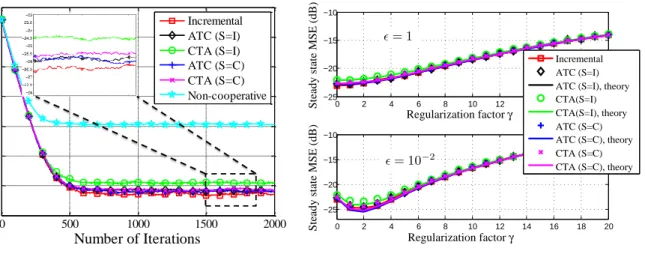
this result is due to (94) withwo there replaced bywˆo. Fig. 2(a) shows the learning curves for different algorithms for γ = 2 and = 10−3. We see that the diffusion and incremental schemes have similar performance, and both of them have about 10 dB gain over the non-cooperation case. To examine the
0 500 1000 1500 2000 -30 -25 -20 -15 -10 -5 0 5 Number of Iterations N e tw ork M S E (dB) Incremental ATC (S=I) CTA (S=I) ATC (S=C) CTA (S=C) Non-cooperative
(a) Learning curves (γ= 2and= 10−3).
0 2 4 6 8 10 12 14 16 18 20 −25 −20 −15 −10 Regularization factor γ
Steady state MSE (dB)
0 2 4 6 8 10 12 14 16 18 20 −25 −20 −15 −10 Regularization factor γ
Steady state MSE (dB)
Incremental ATC (S=I) ATC (S=I), theory CTA(S=I) CTA(S=I), theory ATC (S=C) ATC (S=C), theory CTA (S=C) CTA (S=C), theory ²= 1 ²= 10−2 (b) Steady-state MSD (µ= 10−3). Fig. 2. Transient and steady-state performance of distributed estimation with sparse parameters.
impact of the parameter and the regularization factor γ, we show the steady-state MSE for different values ofγ andin Fig. 2(b). Whenis small (= 10−2), adding a reasonable regularization (γ = 1∼4) decreases the steady-state MSE. However, when is large (= 1), expression (113) is no longer a good approximation for kwk1, and regularization does not improve the MSE.
B. Distributed Collaborative Localization
The previous example deals with a convex cost (112). Now, we consider a localization problem that has a non-convex cost function and apply the same diffusion strategies to its solution. Assume each node is interested in locating a common target located atwo = [0 0]T. Each node kknows its positionx
k and has a noisy measurement of the squared distance to the target:
dk(i) =kwo−xkk2+zk(i), k= 1,2, . . . , N
where zk(i) ∼ N(0, σz,k2 ) is the measurement noise of node k at time i. The component cost function
Jk(w) at node k is chosen as Jk(w) = 1 4E dk(i)− kw−xkk2 2 (120)
where we multiply by1/4here to eliminate a factor of4that will otherwise appear in the gradient. If each node k minimizes Jk(w) individually, it is not possible to solve for wo. Therefore, we use information from other nodes, and instead seek to minimize the following global cost:
Jglob(w) = 1 4 N X Edk(i)− kw−xkk2 2 (121)
This problem arises, for example, in cellular communication systems, where multiple base-stations are interested in locating users using the measured distances between themselves and the user. Diffusion algorithms (18) and (19) can be applied to solve the problem in a distributed manner. Each nodekwould update its estimate of wo by using the gradient vectors of{Jl(w)}
l∈Nk, which are given by:
∇wJl(w) =−Edl(i) (w−xl) +kw−xlk2(w−xl) (122)
However, the nodes are assumed to have access to measurements {dl(i), xl} and not to Edl(i). In this case, nodes can use the available measurements to approximate the gradient vectors in (24) and (25) as:
b
∇wJl(w) =−dl(i)(w−xl) +kw−xlk2(w−xl) (123)
If we do not exchange the local gradients with neighbors, i.e., if we set S = I, then the base-stations only share the local estimates of the target position wo with their neighbors (no exchange of {x
l}l∈Nk).
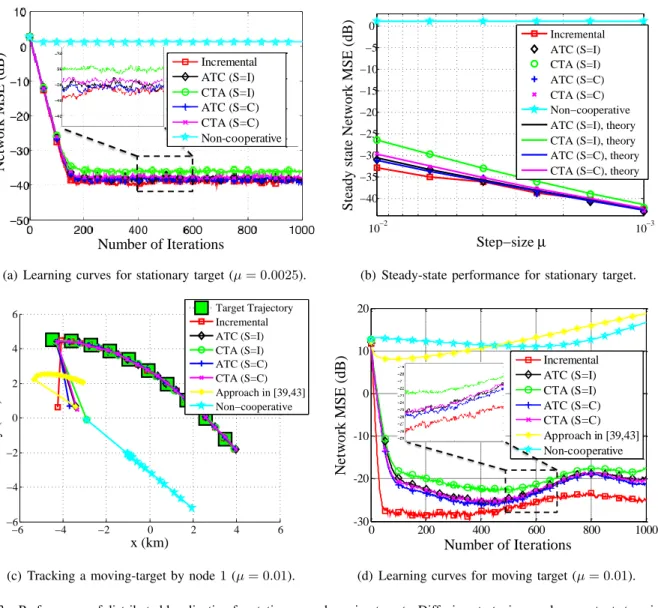
We first simulate the stationary case, where the target stays atwo. In Fig. 3(a), we show the MSE curves for non-cooperative, ATC, CTA, and incremental algorithms. The noise variance is set to σ2
z,k= 1. We set the step-sizes to µ= 0.0025/N for the incremental algorithm, andµ= 0.0025for other algorithms. For ATC and CTA strategies, we use simple averaging for the combination step {al,k}, and for ATC and CTA with gradient exchange, we use Metropolis weights for {cl,k} to combine the gradients. The performance of CTA and ATC algorithms are close to each other, and both of them are close to the incremental scheme. In Fig. 3(b), we show the steady state MSE with respect to different values of µ. We also use expression (110) to evaluate the theoretical performance of the diffusion strategies. As the step-size becomes small, the performances of diffusion and incremental algorithms are close, and the MSE decreases as µ decreases. Furthermore, we see that exchanging only local estimates (S = I) is enough for localization, compared to the case of exchanging both local estimates and gradients (S=C). Next, we apply the algorithms to a non-stationary scenario, where the target moves along a trajectory, as shown in Fig. 3(c). The step-size is set to µ = 0.01 for diffusion algorithms, and to µ = 0.01/N
for the incremental approach. To see the advantage of using a constant step-size for continuous tracking, we also simulate the vanishing step-size version of the algorithm from [39], [43] (µk,i = 0.01/i). The diffusion algorithms track well the target but not the non-cooperative algorithm and the algorithm from [39], [43], because a decaying step-size is not helpful for tracking. The tracking performance is shown in Fig. 3(d).
0 500 1000 1500 2000 -30 -25 -20 -15 -10 -5 0 5 Number of Iterations A ve ra ge N e tw ork M S E (dB) Incremental ATC (S=I) CTA (S=I) ATC (S=C) CTA (S=C) Non-cooperation 0 500 1000 1500 2000 -30 -25 -20 -15 -10 -5 0 5 Number of Iterations A ve ra ge N e tw ork M S E (dB) Incremental ATC (S=I) CTA (S=I) ATC (S=C) CTA (S=C) Non-cooperation 0 500 1000 1500 2000 -30 -25 -20 -15 -10 -5 0 5 Number of Iterations N e tw ork M S E (dB) Incremental ATC (S=I) CTA (S=I) ATC (S=C) CTA (S=C) Non-cooperation 0 500 1000 1500 2000 -30 -25 -20 -15 -10 -5 0 5 Number of Iterations N e tw ork M S E (dB) Incremental ATC (S=I) CTA (S=I) ATC (S=C) CTA (S=C) Non-cooperative
(a) Learning curves for stationary target (µ= 0.0025).
10−3 10−2 −40 −35 −30 −25 −20 −15 −10 −5 0 Step−size µ
Steady state Network MSE (dB)
Incremental ATC (S=I) CTA (S=I) ATC (S=C) CTA (S=C) Non−cooperative ATC (S=I), theory CTA (S=I), theory ATC (S=C), theory CTA (S=C), theory
(b) Steady-state performance for stationary target.
−6 −4 −2 0 2 4 6 −6 −4 −2 0 2 4 6 x (km) y (km) Target Trajectory Incremental ATC (S=I) CTA (S=I) ATC (S=C) CTA (S=C) Approach in [39,43] Non−cooperative
(c) Tracking a moving-target by node1(µ= 0.01).
0 200 400 600 800 1000 -30 -20 -10 0 10 20 Number of Iterations N e tw ork M S E (dB) Incremental ATC (S=I) CTA (S=I) ATC (S=C) CTA (S=C) Approach in [39,43] Non-cooperative
(d) Learning curves for moving target (µ= 0.01). Fig. 3. Performance of distributed localization for stationary and moving targets. Diffusion strategies employ constant step-sizes, which enable continuous adaptation and learning even when the target moves (which corresponds to a changing cost function).
VI. CONCLUSION
This paper proposed diffusion adaptation strategies to optimize global cost functions over a network of nodes, where the cost consists of several components. Diffusion adaptation allows the nodes to solve the distributed optimization problem via local interaction and online learning. We used gradient approximations and constant step-sizes to endow the networks with continuous learning and tracking abilities. We analyzed the mean-square-error performance of the algorithms in some detail, including their transient and steady-state behavior. Finally, we applied the scheme to two examples: distributed sparse parameter estimation and distributed localization. Compared to incremental methods, diffusion
strategies do not require a cyclic path over the nodes, which makes them more robust to node and link failure.
APPENDIXA
PROOF OFMEAN-SQUARESTABILITY Taking the ∞−norm of both sides of (79), we obtain
kWik∞ ≤ kP2TΓP1Tk∞·kWi−1k∞+σ2vkSk21·kP2Tk∞·kΩk2∞ ≤ kP2Tk∞· kΓk∞· kP1Tk∞· kWi−1k∞ +σv2kSk21· kP2Tk∞· kΩk2∞ =kΓk∞·kWi−1k∞+ max 1≤k≤Nµ 2 k ·σ2vkSk21 (124)
where we used the fact that kPT
1 k∞ =kP2Tk∞= 1 because each row of P1T and P2T sums up to one. Moreover, from (76), we have
kΓk∞= max 1≤k≤N(γ 2 k+µ2kαkSk21) (125) Iterating (124), we obtain kWik∞ ≤ kΓki∞· kW0k∞ + max 1≤k≤Nµ 2 k ·σv2kSk21 i−1 X j=0 kΓkj∞ (126)
We are going to show further ahead that condition (80) guaranteeskΓk∞<1. Now, given thatkΓk∞<1,
the first term on the right hand side of (126) converges to zero as i→ ∞, and the second term on the right-hand side of (126) converges to:
lim i→∞σ 2 vkSk21 i−1 X j=0 kΓkj ∞= σ2 vkSk21 1− kΓk∞ (127)
Therefore, we establish (82) as follows:
lim sup i→∞ kWik∞≤ max 1≤k≤Nµ 2 k · σ 2 vkSk21 1− kΓk∞ = max 1≤k≤Nµ 2 k ! · kSk21σ2v 1− max 1≤k≤N(γ 2 k+µ2kαkSk21) (128)
The only fact that remains to prove is to show that (80) ensures kΓk∞ <1. From (125), we see that
the condition kΓk∞<1is equivalent to requiring:
γk2+µ2kαkSk21 <1, k= 1, . . . , N. (129)
Then, using (65), this is equivalent to:
1−µk N X l=1 sl,kλl,max 2 +µ2kαkSk21<1 (130) 1−µk N X l=1 sl,kλl,min 2 +µ2kαkSk21 <1 (131)
fork= 1, . . . , N. Recalling the definitions forσk,max andσk,min in (81) and solving these two quadratic inequalities with respect toµk, we arrive at:
0< µk< 2σk,max σ2 k,max+αkSk21 , 0< µk< 2σk,min σ2 k,min+αkSk21 and we are led to (80).
APPENDIX B
BLOCKMAXIMUMNORM OF AMATRIX
Consider a block matrix X with blocks of size M×M each. Its block maximum norm is defined as [35]: kXkb,∞,max x6=0 kXxkb,∞ kxkb,∞ (132)
where the block maximum norm of a vectorx,col{x1, . . . , xN}, formed by stackingN vectors of size
M each on top of each other, is defined as [35]:
kxkb,∞, max
1≤k≤Nkxkk (133)
where k · k denotes the Euclidean norm of its vector argument.
Lemma 4 (Block maximum norm). If a block diagonal matrix X ,diag{X1, . . . , XN} ∈ RN M×N M consists ofN blocks along the diagonal with dimensionM×M each, then the block maximum norm of X is bounded as
kXkb,∞≤ max
1≤k≤NkXkk (134)
Proof:Note that Xx= col{X1x1,. . . ,XNxN}. Evaluating the block maximum norm of vectorXxleads to kXxkb,∞= max 1≤k≤NkXkxkk ≤ max 1≤k≤NkXkk · kxkk ≤ max 1≤k≤NkXkk ·1max≤k≤Nkxkk (135) Substituting (135) and (133) into (132), we establish (134) as
kXkb,∞,max x6=0 kXxkb,∞ kxkb,∞ ≤max x6=0 max1≤k≤NkXkk ·max1≤k≤Nkxkk max1≤k≤Nkxkk = max 1≤k≤NkXkk (136)
Next, we prove that, if all the diagonal blocks of X are symmetric, then equality should hold in (136). To do this, we only need to show that there exists an x0 6= 0, such that
kXx0kb,∞
kx0kb,∞
= max
1≤k≤NkXkk (137)
which would mean that
kXkb,∞,max x6=0 kXxkb,∞ kxkb,∞ ≥ kXx0kb,∞ kx0kb,∞ = max 1≤k≤NkXkk (138)
Then, combining inequalities (136) and (138), we would obtain desired equality that
kXkb,∞= max
1≤k≤NkXkk (139)
when X is block diagonal and symmetric. Thus, without loss of generality, assume the maximum in (137) is achieved by X1, i.e.,
max
1≤k≤NkXkk=kX1k
For a symmetricXk, its 2-induced normkXkk(defined as the largest singular value ofXk) coincides with the spectral radius ofXk. Letλ0denote the eigenvalue ofX1of largest magnitude, with the corresponding right eigenvector given by z0. Then,
max
We selectx0= col{z0,0, . . . ,0}. Then, we establish (137) by: kXx0kb,∞ kx0kb,∞ = kcol{X1z0,0, . . . ,0}kb,∞ kcol{z0,0, . . . ,0}kb,∞ = kX1z0k kz0k = kλ0z0k kz0k =|λ0|= max 1≤k≤NkXkk APPENDIX C STABILITY OFBANDF Recall the definitions of the matrices B andF from (93) and (100):
B=P2T[IM N− MD∞]P1T (140) F =P1[IM N − MD∞]P2 ⊗P1[IM N− MD∞]P2 =BT ⊗ BT (141)
From (140)–(141), we obtain (see Theorem 13.12 from [57, p.141]):
ρ(F) =ρ(BT ⊗ BT) = [ρ(BT)]2= [ρ(B)]2 (142)
where ρ(·) denotes the spectral radius of its matrix argument. Therefore, the stability of the matrixF is equivalent to the stability of the matrix B, and we only need to examine the stability of B. Now note that the block maximum norm (see the definition in Appendix B) of the matrix B satisfies
kBkb,∞≤ kIM N− MD∞kb,∞ (143)
since the block maximum norms ofP1 andP2 are one (see [35, p.4801]):
P1T b,∞= 1, P2T b,∞= 1 (144)
Moreover, by noting that the spectral radius of a matrix is upper bounded by any matrix norm (Theorem 5.6.9, [50, p.297]) and that IM N − MD∞ is symmetric and block diagonal, we have
ρ(B)≤ kIM N− MD∞kb,∞=ρ(IM N− MD∞) (145)
Therefore, the stability of B is guaranteed by the stability of IM N − MD∞. Next, we call upon the
following lemma to bound kIM N−MD∞kb,∞.
Lemma 5 (Norm of IM N−MD∞). It holds that the matrix D∞ defined in (90) satisfies
whereγk is defined in (65).
Proof: Since D∞ is block diagonal and symmetric, IM N− MD∞ is also block diagonal with blocks
{IM−µkDk,∞}, where Dk,∞ denotes the kth diagonal block ofD∞. Then, from (134) in Lemma 4 in
Appendix B, it holds that
kIM N−MD∞kb,∞= max
1≤k≤NkIM−µkDk,∞k (147) By the definition of D∞ in (90), and using condition (45) from Assumption 1, we have
N X l=1 sl,kλl,min ! ·IM ≤ Dk,∞≤ N X l=1 sl,kλl,max ! ·IM
which implies that
IM −µkDk,∞≥ 1−µk N X l=1 sl,kλl,max ! ·IM (148) IM −µkDk,∞≤ 1−µk N X l=1 sl,kλl,min ! ·IM (149)
Thus, kIM−µkDk,∞k ≤γk. Substituting into (147), we get (146).
Substituting (146) into (145), we get:
ρ(B)≤ max
1≤k≤Nγk (150)
As long as max
1≤k≤Nγk<1, then all the eigenvalues of B will lie within the unit circle. By the definition ofγk in (65), this is equivalent to requiring
|1−µkσk,max|<1, |1−µkσk,min|<1
for k = 1, . . . , N, where σk,max and σk,min are defined in (81). These conditions are satisfied if we chooseµk such that
0< µk<2/σk,max, k= 1, . . . , N (151)
which is obviously guaranteed for sufficiently small step-sizes (and also by condition (80)).
REFERENCES
[1] J. Chen, S.-Y. Tu, and A. H. Sayed, “Distributed optimization via diffusion adaptation,” in Proc. IEEE International Workshop on Comput. Advances Multi-Sensor Adaptive Process. (CAMSAP), Puerto Rico, Dec. 2011, pp. 281–284. [2] J. Chen and A. H. Sayed, “Performance of diffusion adaptation for collaborative optimization,” inProc. IEEE International