Highway Asset Management
By
Chao Yang
A Doctoral Thesis
Submitted in partial fulfilment of the requirements for the award of Doctor of Philosophy of the University of Nottingham
Abstract
The aim of this thesis is to provide a framework for a decision making system to operate a highway network, to evaluate the impacts of maintenance activities, and to allocate limited budgets and resources in the highway network. This integrated model is composed of a network level traffic flow model (NTFM), a pavement deterioration model, and an optimisation framework.
NTFM is applicable for both motorway and urban road networks. It forecasts the traffic flow rates during the day, queue propagation at junctions, and travel delays throughout the network. It uses sub-models associated with different road and junction types which typically comprise the highway. To cope with the two-way traffic flow in the network, an iterative algorithm is utilised to generate the evolution of dependent traffic flows and queues. By introducing a reduced flow rate on links of the network, the effects of strategies employed to carry out roadworks can be mimicked. In addition, a traffic rerouting strategy is proposed to model the driver behaviour, i.e. adjusting original journey plans to reduce journey time when traffic congestion occurs in the road network. A pavement age gain model was chosen as the pavement deterioration model, which is used to evaluate the current pavement condition and predict the rate of pavement deterioration during the planning period. It deploys pavement age gain as the pavement improvement indicator which is simple and easy to apply. Moreover, the deterministic pavement age gain model can be transformed to a probabilistic one, using the normal distribution to describe the stochastic nature of pavement deterioration.
A multi-objective and multi-constraint optimisation model was constructed to achieve the best pavement maintenance and rehabilitation (M&R) strategy at the network level. The improved non-dominated sorting genetic algorithm (NSGA-II) is applied to perform system optimisation. Furthermore, the traffic operations on worksites, i.e. lane
closure options, start time of the maintenance, and traffic controls, are investigated so as to prevent, or at least to reduce, the congestion that resulted from maintenance and reconstruction works.
The case studies indicated that NTFM is capable of identifying the relationship between traffic flows in the network and capturing traffic phenomenon such as queue dynamics. The maintenance cost is reduced significantly using the developed optimisation framework. Also, the cost to the road users is minimised by varying the worksite arrangements. Consequently, the integrated decision making system provides highways agencies with the capability to better manage traffic and pavements in a highway network.
Keywords: NTFM, iterative algorithm, traffic rerouting strategy, optimisation, genetic algorithms, M&R strategy, NSGA-II, worksite arrangements
Acknowledgements
First and foremost, I would like to express my sincere appreciation and gratitude to my supervisors, Prof. John Andrews, Dr. Rasa Remenyte-Prescott, and Dr. Matthew Byrne, for their inspiring guidance and encouragement throughout the research as well as for always being friendly and helpful.
I would like to extend my thanks to other members of Infrastructure Asset Management Group and the people of the Nottingham Transportation Engineering Centre for their assistance, encouragement and friendship.
Finally, I wish to thank my parents and sister for their endless inspiration, constant support and understanding during the research.
Abbreviations
AADT Annual Average Daily Traffic ARRB Australian Road Research Board BGA Binary-coded Genetic Algorithm CTM Cell Transmission Model
D Diverge junction
D2AP Dual 2 lane Carriageway D3M Dual 3 lane Motorway GAs Genetic Algorithms
HDM-4 Highway Development and Management model LWR
MG Merge junction
Lighthill, Whitham and Richards
MOGA Multi-Objective Genetic Algorithm M&R Maintenance and Rehabilitation
NSGA Non-dominated Sorting Genetic Algorithm NTFM Network level Traffic Flow Model
O-D Origin-Destination
Ov Overlay
PCI Pavement Condition Index PCU Passenger Car Unit
PMS Pavement Management System PSI Pavement Serviceability Index
R Roundabout
Re Resurfacing
S On-ramps and Off-ramps S2 Single Carriageway SD Surface Dressing SI Signalized Intersection SR Signalized Roundabout ST Signalized T-junction
I
Contents
1 Introduction ... 1 1.1 Background ... 2 1.1.1 Highway Networks ... 2 1.1.2 Road Classes ... 21.1.3 Traffic Related Organisations ... 3
1.2 Objectives ... 3
1.3 Contributions of this Thesis ... 4
2 Literature Review on Traffic Modelling ... 6
2.1 Introduction ... 6
2.2 Traffic Models ... 6
2.2.1 Macroscopic Traffic Flow Models ... 7
2.2.2 Priority Junction Models ... 9
2.3 Traffic Rerouting Control Approaches ... 12
2.4 Summary ... 14
3 Network Level Traffic Flow Model ... 16
3.1 Introduction ... 16
3.1.1 Network Representation ... 17
3.1.2 Model Data ... 18
3.1.3 Main Principle of NTFM... 19
3.2 Junction Sub-models ... 23
3.2.1 Signalized Intersection Model ... 24
3.2.2 T-junction Model ... 27
3.2.3 Signalized T-junction Model ... 31
3.2.4 Roundabout Model ... 32
3.2.5 Signalized Roundabout Model ... 43
3.2.6 On-ramp and Off-ramp Models ... 44
3.2.7 Merge and Diverge Models ... 46
3.2.8 Roadwork Node Model ... 48
3.3 Link Model ... 50
3.3.1 Calculation of Travel Duration ... 51
II
3.3.3 Extension for Multi-lane Link ... 54
3.3.4 Extension for Roadwork ... 57
3.4 Highway Network Performance Metrics ... 58
3.5 Network Solution Routine ... 60
3.5.1 Convergence of In Profiles and Out Profiles... 60
3.5.2 Forecast of Traffic Condition ... 61
3.6 Case Study ... 63
3.6.1 Network Simulation ... 64
3.6.2 Evaluation of Traffic Condition ... 64
3.6.3 Discussion ... 68
3.7 Traffic Rerouting Strategy ... 69
3.7.1 Introduction ... 69
3.7.2 Methodology ... 69
3.7.3 Case Study ... 75
3.8 Summary ... 82
4 Literature Review on Highway Asset Modelling ... 83
4.1 Introduction ... 83
4.2 M&R Operations for Pavement ... 84
4.2.1 Minor Maintenance ... 85
4.2.2 Surface Treatments ... 85
4.2.3 Major Maintenance ... 86
4.3 Decision Making Strategies for M&R ... 87
4.3.1 M&R Prioritisation Model ... 88
4.3.2 M&R Optimisation Model ... 90
4.4 Genetic Algorithms ... 94
4.4.1 Introduction ... 94
4.4.2 Simple Genetic Algorithms ... 95
4.4.3 Multi-objective Genetic Algorithms ... 101
4.5 Summary ... 112
5 Scheduling of Pavement Maintenance ... 114
5.1 Introduction ... 114
5.2 Scheduling of Pavement Maintenance using NSGA-II at the Network Level ... 115
5.2.1 Age Gain Maximisation Model ... 115
III
5.2.3 Model Formulation ... 118
5.2.4 Case Study ... 120
5.2.5 Probabilistic Pavement Deterioration Model ... 133
5.3 Scheduling of Pavement Maintenance using the NTFM at the Project Level ... 141
5.3.1 Methodology ... 142
5.3.2 Case Study ... 148
5.4 Maintenance Planning using the NTFM in the Long-term ... 156
5.5 Maintenance Planning by Balancing between Maintenance Costs and Road User Costs ... 159
5.6 Summary ... 162
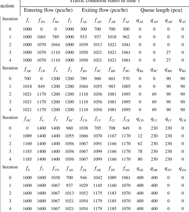
6 Model Application to the Loughborough-Nottingham Network ... 164
6.1 Loughborough-Nottingham Highway Network ... 164
6.2 Model Calibration ... 168
6.2.1 Network Calibration ... 168
6.2.2 Available Traffic Flow Data ... 168
6.2.3 Movement of Traffic Flow ... 169
6.3 The Evaluation of Traffic Condition ... 170
6.3.1 Highway Network Performance under Normal Conditions ... 170
6.3.2 The Implementation of Roadworks ... 182
6.3.3 Discussion ... 188
6.4 Maintenance Planning for Road Sections in the Long-term ... 189
6.4.1 Dual Carriageway (MG2-R4) ... 189
6.4.2 Single Carriageway (SR2-R4) ... 194
6.4.3 Motorway (S4-S7) ... 196
6.4.4 Dual Carriageway (SI1-ST2) ... 198
6.4.5 Motorway (S2-S3) ... 200
6.4.6 Discussion ... 201
6.5 Maintenance Planning for the Road Sections in the Short-term ... 202
6.5.1 Possible Maintenance Arrangements on Dual Carriageway (MG2-R4) ... 202
6.5.2 Optimisation of Maintenance Arrangements on Dual Carriageway (MG2-R4) . 204 6.5.3 Optimisation of Maintenance Arrangements on Single Carriageway (SR2-R4) 207 6.5.4 Discussion ... 209
6.6 Summary ... 209
IV
7.1 Summary ... 211
7.2 Sensitivity of Main Assumptions ... 213
7.2.1 Junction model ... 213
7.2.2 Queue model ... 215
7.2.3 Pavement deterioration model ... 216
7.2.4 Road user cost ... 216
7.2.5 Maintenance implementation ... 217
7.3 Conclusions ... 217
7.4 Future Model Validation ... 218
7.5 Future Work ... 219
References ... 221
Appendix A: Flow Diagram of NTFM ... 230
Appendix B: Practical Implementation and Computational Time of the Decision Making System ... 233
1
1
Introduction
Since the late-1980s, more than 90% of motorised passenger travel and around 65% of domestic freight in the UK have been delivered on the highway network. The total road length of highway networks in the UK was estimated to be 245,000 miles in 2010 [1]. Also, the total road length in the UK has increased by about 2,500 miles in the decade since 2000, approximately 1% per year. It demonstrates that the highways authorities have shifted its attention from construction of new roads to the maintenance and rehabilitation of existing ones. According to the Annual Local Authority Road Maintenance Survey [2], in England, the government has spent heavily on road maintenance in recent years. £2,240m was spent in 2006, £937m in 2007 and another £861m in 2008, an aggregate total of £6,867m from 2002 to 2008, in order to maintain the serviceability level of pavements.
3
The survey also reports that a further £10.65b is currently required to bring the UK’s roads to the desired standard. In addition to the expenditure on carrying out the work, the travel delay cost to the road users caused by maintenance is significant and expected to substantially exceed the corresponding cost of maintenance [ ].
In this thesis a framework of decision making system is developed. Its purpose is to assist the highways agencies in operating the highway network, predicting traffic characteristics in the network, preventing, or at least reducing, traffic congestion, maintaining the pavement condition at a serviceable level, identifying the maintenance requirements, and minimising both maintenance and road user costs.
2
1.1 Background
1.1.1 Highway Networks
The highway network in the UK is comprised of motorways, ‘A’ roads, rural minor roads and urban minor roads. Motorways are usually used by long-distance traffic, while ‘A’ roads are used by both medium-distance and long-distance traffic. As for the short-distance traffic, urban minor roads and rural minors are employed. Motorways and ‘A’ roads occupied 1% and 12% respectively of the total road length of the highway network in the UK, while rural minor roads and urban roads accounted for the remaining 54 % and 33%. Nonetheless, 19.8% of the total transportation volume was conveyed on motorways and 44.3% on ‘A’ roads.
1.1.2 Road Classes
To distinguish the purposes and functions of different kind of roads, the road classes adopted in UK are listed in Table 1-1 [4]:
Table 1-1: COBA Road classes
Road class Description Speed limit (mph)
1 Rural single carriageway 70
2 Rural all-purpose dual 2 lane carriageway 70 3 Rural all-purpose dual 3 or more lane carriageway 70 4 Motorway (urban or rural), dual 2 lanes 70 5 Motorway (urban or rural), dual 3 lanes 70 6 Motorway (urban or rural), dual 4 or more lanes 70 7 Urban road, Non-central, single or dual carriageway 30 8 Urban road, Central, single or dual carriageway 30 9 Small town road, single or dual carriageway 30 or 40 10 Suburban main road, single carriageway 40 11 Suburban main road, dual carriageway 40
3
The COBA (COst Benefit Analysis) software can be used to compare the costs of road projects with benefits derived by road user costs. Classes 1 to 6 are recognised as all-purpose roads (‘A’ roads) and motorways that are generally restricted by the maximum speed, 70 mph. The traffic flow model developed in this thesis works with average speeds which are not allowed to exceed the specified speed limits. Further, the flow capacity for each road class as stated in Table 1-1 is depicted in Table 1-2 [5]:
Table 1-2: Default road capacity
Road class Capacity (pcu/hr/standard lane)
1 1400
2 and 3 1800 4, 5 and 6 2000 7, 8, 9 and 10 1400
11 1800
1. “pcu” stands for passenger car unit, which is used to express highway capacity. For example, one car is recognised as a single unit, motorcycle is considered as half unit, heavy vehicles are considered as more than 3 units.
1.1.3 Traffic Related Organisations
In England, the Highways Agency (HA) is responsible for managing motorways and trunk roads, whereas other roads are run by the local authorities, e.g. Nottingham County Council. While in Scotland and Wales, roads are operated by Transport Scotland and the Welsh Assembly Government, respectively. As for Northern Ireland, roads are the responsibility of Roads Service Northern Ireland.
1.2 Objectives
The aim of this thesis is to develop an integrated decision making system to forecast and operate traffic flows, evaluate the impacts of different maintenance activities, and allocate limited budgets and resources in a highway network. This system will be
4
utilized to facilitate traffic on the network and to maintain the pavement service level to ensure optimal performance. To fulfil this aim, the following specific objectives are considered:
• To construct a macroscopic traffic flow model for identifying the traffic characteristics in a highway network.
• To develop a traffic rerouting strategy based on the proposed traffic model for modeling driver behavior when traffic congestion takes place in the highway network, i.e. divert traffic heading to the congested areas to take alternative routes and avoid traffic delays.
• To select an appropriate pavement deterioration model to evaluate pavement condition during the planning period.
• To derive all combinations of maintenance and rehabilitation actions that can be applied to the network and model their effects.
• To develop a genetic algorithm-based optimization technique for pavement maintenance management. The optimization technique will be used to achieve the optimal pavement maintenance and rehabilitation strategy with the purpose of minimising maintenance cost and user cost and maximising pavement condition.
In summary, this thesis provides a framework and the sub-models to improve network performance, enhance pavement serviceability, and minimise maintenance cost and road user cost.
1.3 Contributions of this Thesis
5
• A novel network level traffic flow model (NTFM) is built and the software developed that is applicable for an integrated motorway and urban road network, in which two-way traffic flow is predicted using an iterative simulation method. More junction types are taken into account by NTFM than the existing integrated traffic flow models.
• A roadwork node sub-model is introduced to NTFM, which is used to evaluate the traffic conditions in a highway network under normal conditions and different maintenance scenarios.
• A traffic rerouting strategy is developed to model driver behavior when traffic congestion takes place in the highway network.
• An optimisation technique is built that allows for the selection and scheduling of maintenance and rehabilitation operations for road sections on a highway network.
• NTFM is utilised to optimise maintenance cost and road user cost together with pavement deterioration models in both long-term and short-term, where Genetic Algorithms are employed to perform optimisation.
• Overall, the capability of the model is to help highway engineers to make more effective decisions in terms of the limited annual budgets as well as the frequencies of maintenance activities.
6
2
Literature Review on Traffic Modelling
2.1 Introduction
The modelling of traffic flow in highway networks is of vital importance for pavement management, providing information for traffic control, traffic flow prediction, traffic diversion, and the implementation of roadwork. In this chapter, the literature on the traffic flow models will be discussed first. Since traffic rerouting techniques are for reducing excessive congestion, and, making more efficient use of the existing roads, the second part of the literature review will be devoted to that area.
2.2 Traffic Models
Typically, traffic flow models are categorised into two main groups: macroscopic models and microscopic models. Macroscopic traffic models are used to identify the aggregate behaviour of sets of vehicles, easy to validate and ensure a good real-time quality, such as the fluid-dynamic traffic models [6, 7]. Microscopic models are applied to model the travel behaviour of an individual vehicle which is recognised as a function of the traffic conditions in its environment [8, 9]. As drivers’ behaviour in real traffic is difficult to observe and measure, microscopic models are difficult to validate accurately [10]. In addition, the computational effort required by microscopic models is significantly higher than that for macroscopic models and the data required by microscopic models are harder to get. As for macroscopic models, they do not distinguish their components flows by origins and destinations; therefore when the traffic stream arrives at junctions, macroscopic models usually assign fixed turning ratios for the traffic stream [10]. In this thesis, focus is on macroscopic models.
7 2.2.1 Macroscopic Traffic Flow Models
During the past decades, a number of macroscopic traffic models have been constructed to identify traffic behaviour on motorways and urban roads. Lighthill and Whitham [6] and Richards [7]
As an extension to LWR model,
provided a pioneering flow-dynamic model based on first-order differential equations, termed the LWR model, which was the first model used to describe unidirectional traffic flow on highway networks.
Payne [11] developed a second-order model [12]
Daganzo [10
based on the car-following model [13] that considered the driver’s reaction time. This results in a dynamic mean speed equation rather than the static one applied in first-order models, in which the dynamic flow phenomena, i.e. emergent traffic congestion and stop-and-go traffic, are modelled. Because first-order models and second-order models are mainly focused on the traffic characteristics on road links, they would only be sufficient for signalized networks where the traffic interaction among flows from competing arms is eliminated.
] developed a cell transmission model (CTM) that adopted a convergent approximation to the LWR model to evaluate the traffic on a highway network with a single entrance and exit. Afterwards, Daganzo [14] applied merge cell and diverge cell in a CTM to generalise the junctions within a highway network. CTM can be used to reproduce kinematic waves, the formation and dissipation of a queue in an explicit manner, in both congested and uncongested regimes, and to model the traffic movement on a simple highway network with three-legged junctions. Lo [15] introduced signal control to CTM, and Lo et al. [16] further developed signalized merge and diverge cells in CTM to broaden its applicability. However, priority junctions, i.e. T-junction and roundabout, are not considered, so the conflicting requirements of the traffic flows from
8
competing directions cannot be captured. Thus it is only suitable for signalized networks.
Messmer and Papageorgiou [17] considered the situation of a motorway network based on the second-order traffic flow model, METANET model. The approach has been widely applied to simulate traffic flow phenomena on motorway networks of arbitrary characteristics, including motorway links, on-ramps and off-ramps (slip roads). Other research has been performed to improve METANET, the adoption of variable speed limits on motorways is described in Breton, et al. [18] and Hegyi, et al. [19], and the application of route guidance is depicted in Deflorio [20] and Karimi et al. [21]. Subsequently, Van den Berg et al. [22] developed an integrated traffic control capability for mixed urban and motorway networks, as motorway traffic is heavily influenced by the traffic flows on the connected urban roads, and vice versa. This model is composed of the METANET model that was used to evaluate motorway traffic and a queue length model based on the Kashani model [23] for urban traffic, coupled via on-ramps and off-ramps. However, these studies referred to METANET do not identify the traffic interaction among competing flows, since the inflow and outflow for each node in METANET is only characterised by turning ratios of traffic flows from each link that is connected to the node. In Van den Berg et al. [22], the traffic in the major road and the slip road for an on-ramp are treated separately. They need to be addressed dependently since traffic from slip road is also restricted by the traffic on the major road. Also, the updated urban traffic model assigns sub-queues for each turning direction on road link; however, shared lanes are not taken into account where traffic heading to different directions might be mixed together.
9 2.2.2 Priority Junction Models
Many different approaches for evaluation of traffic at unsignalized intersections have been presented and investigated, including gap acceptance theory, and queuing theory. 2.2.2.1 Gap Acceptance Theory
In traditional gap acceptance models, it has been assumed that the vehicles in the major stream have absolute priority over the vehicles in the minor stream. It means that the major stream is unaffected by the minor stream vehicles. Within unsignalized intersection theory, it is also assumed that drivers are both consistent and homogenous [24]. A consistent driver is assumed to act the same way every time in all similar situations. For a homogeneous traffic stream, all drivers are supposed to behave in the same way.
In the gap acceptance theory two major parameters are investigated, critical gap and follow-up time. The critical gap is the minimum gap for drivers in the minor stream to accept and enter the intersection, any shorter gap will be rejected and any longer gap accepted. The follow-up time is the headway between two departing minor stream vehicles in very long gaps. Many techniques have been applied to estimate the critical gaps at unsignalized intersections. Some of the important methods are examined in [24] and [25], and a set of quality criteria has been formulated by which the usefulness of each method is appraised [25]. Furthermore, Brilon et al. [25] found that the maximum likelihood method [26] and Hewitt’s method [27] are superior to other methods for estimating the critical gap.
In addition, the capacity at the unsignalized intersection is very important. Capacity on the minor road is determined as the maximum number of minor stream vehicles that can cross the intersection during a unit time under predefined conditions. In 1973, Siegloch [28] developed the fundamental capacity equation of the minor road. Based on this
10
equation, numerous capacity formulas are computed using different headway models [24]. The distribution of headway is essential for the calculation of capacity at unsignalized intersections, including negative exponential distribution (M1), shifted exponential distribution (M2) and dichotomized distribution (M3) [29]. The M3 model allows a portion of the vehicles to be bunched and the remaining vehicles are free vehicles that move without interacting with the front vehicles, where the latter is characterised by a shifted exponential distribution. A more practical M3 model is proposed by Cowan [29], which does not attempt to model the bunched vehicles as their headways are not accepted by minor stream vehicles but rather model the larger gaps between the free vehicles. Based on Cowan’s M3 headway model, Plank and Catchpole [30] derived the corresponding capacity formula using Siegloch’s capacity equation [28].
Kimber [31] found that the vehicles in the minor stream could also affect the vehicles in the major steam, especially under high flow circumstances. Thus a new gap acceptance model based on limited priority for the major stream was proposed by Troutbeck and Kako [32], in which the major stream vehicles are expected to be slightly delayed so as to accommodate the merging minor stream vehicles. The limited priority gap acceptance model has been applied to evaluate the merging behaviours at roundabouts [32] and freeway on-ramps [33].
2.2.2.2 Queuing Theory
Starting from the capacity at unsignalized intersections, further traffic parameters, which represent the quality of traffic operations, can be evaluated. Queuing theory is generally used to evaluate situations which involve average delays, average queue lengths, distribution of delays and distribution of queue lengths. In 1962, Tanner [34] established the equations for the average delays for minor stream vehicles at
11
unsignalized intersections with only one major stream and one minor stream. This kind of intersection belongs to the M/G2/1 queuing system [35], M represents the traffic flow arrival pattern of the minor stream, i.e. exponentially distributed headway; G is service time, i.e. the time spent in the first position of the queue. Two types of service times are involved, one is the service time for vehicles entering the empty system and the other is the service time for vehicles joining the queue when other vehicles are already queuing. Finally “1” stands for one service facility, i.e. one service lane for the minor stream. Comparable solutions to the M/G2/1 queuing system have been introduced by Yeo and Weesakul [36] and Kremser [37, 38], who [37] proposed the formulae for the expectations of the two service times. Afterwards, Daganzo [39] and Poeschl [40] have derived new formulae to improve Kremser’s approach. Based on queuing theory, Ning [41] proposed a universal procedure for calculating the capacity for the M/G2/1 queuing system under different predefined conditions, extending the method to cope with the queuing system with more than one major stream.
2.2.2.3 Discussion
One disadvantage for the gap acceptance models is that they have failed to capture conflicts among the major streams. For instance, the right-turning vehicles (for left-side driving, i.e. in the UK) in the major stream have to give way to the vehicles going ahead from the opposing direction, resulting in a queue forming on the major road. It also led to the variation of the headway distributions on the major road so that the original gap acceptance criteria no longer applies [42]. As a result, gap acceptance models are only sufficient for unsignalized intersections under simpler conditions.
In a mixed road network, adjacent signalized intersections can have a significant impact on capacity and performance of unsignalized intersections [43]. On one hand, signalized intersections can group the vehicles into a queue during the red phases, and then result
12
in a cyclic recurrence of a set of long headways (between vehicles departing freely during the green phase) and a set of short headways (between vehicles departing from the queue), thus it is impractical to model the recurrence of headways with gap acceptance theory [43]. On the other hand, signalized intersections can cause the vehicles to arrive at the downstream intersections in platoons, while the gap acceptance models can be applied only when the platoon does not exist [44]. This is because the headways among a platoon are supposed to be shorter than the critical gap that led to no entry for minor stream vehicles. Consequently, the traditional gap acceptance models are not readily applied in network level analysis.
Moreover, the critical gap is difficult to determine and implement for some special conditions, including a two-stage gap-acceptance process, downstream queue spill back, and driver lane preference [26]; and gap acceptance models are not accurate for modelling directional flow [45].
Compared to gap acceptance theory, queuing theory is a more abstract technique for describing driver departure patterns, and it can be more easily applied to measure the delays at more complicated unsignalized intersections [41]. However, it is also constructed based on headway distribution models, thus it suffers the same drawbacks of the gap acceptance theory that resulted from the variation of headway distributions. As gap acceptance theory and queuing theory mainly focused on investigating the traffic at a single intersection, and not accurate for modelling directional flow [45], they are not capable of identifying traffic characteristic at the network level.
2.3 Traffic Rerouting Control Approaches
A number of techniques have been developed previously for routing control in transportation networks: so as to alleviate traffic congestion, which involve user equilibrium assignments and control strategies that are constructed by combining
13
optimal control theory and macroscopic traffic flow models. Messmer and Papageorgiou [46] applied a nonlinear optimisation approach based on the METANET model [17] to handle the route guidance problem in motorway networks, a parallel solution derived in terms of user equilibrium principles [47] has been proposed by Wie et al. [48]. Another method to this problem of integrated control is the application of a linear programming approach as described in Papageorgiou [49] where both motorways and signal-controlled urban roads are considered. Iftar [50], [51] also presented a linear optimisation approach based on a decentralized routing controller to reduce queue build-up for congested highways, the deployed routing controller is decentralized in the manner that the computations for each node on the network are done locally without any information transfer from any other nodes. Van den Berg et al. [22] formulated a model predictive control approach for mixed motorway and urban networks, based on the METANET model [17], Kashani urban network model [23] and improved on-ramp and off-ramp models. A practically integrated control model when both a motorway and a parallel arterial are included in the network was proposed by Chang et al. [52], [53]. On the basis of the previous studies [52-55], Yue et al. [56] proposed an integrated control approach for mixed road networks, in which traffic flow evolution on on-ramps, off-ramps and surface streets, as well as queue propagation, have been explicitly identified. However, this integrated control is only applicable for motorway and signal-controlled urban network, as the effect of conflicting flow from competing routes on the traffic demand of road link is not taken into account.
In addition, some of the existing traffic control strategies are implemented using origin-destination (O-D) trip matrix, which are exposed to the difficulty of collecting accurate O-D information. The reliability of the obtained O-D trip matrix and computational complexity are the two main disadvantages hindering such strategies from being applied
14
broadly. Furthermore, the traffic flow models themselves are very complicated, which makes these control strategies hard to reach the global optimality [57].
2.4 Summary
The literature review showed that there are numerous different techniques for predicting the traffic condition in the network, but that the following deficiencies exist:
a. A review of the existing traffic flow models indicated that CTM and METANET are widely adopted in traffic management. However, both the models failed to capture the traffic movement taking place at the priority junction.
b. Only limited junction types are taken into account by CTM and METANET, it means that the traffic interaction experienced at some junction types, i.e. signalized T-junction and roundabout, cannot be identified, especially not suitable for the integrated motorway and urban road network that composed of different kinds of junctions.
c. As for priority junctions, the most common methods are gap acceptance theory and queuing theory. They have been applied to investigate the traffic at different kinds of priority junctions. Nevertheless, they become inefficient when modelling directional flow and identifying traffic behaviours at the network level.
d. Based on the proposed traffic models, numerous traffic rerouting control measures have been developed. Most of the control measures take advantage of O-D matrix to describe the modification of journey plans, which require abundant information on individual journey plans.
Considering the traffic interaction at both signalized and priority junctions, this thesis describes a macroscopic traffic flow model the purpose of which is to provide a method for predicting the traffic flow and travel delay for each junction in the network. One
15
feature of this model is that both motorway junctions and urban junctions are evaluated based on the principle of a maximum capacity flow rate at these junctions where flows compete. Another feature is that this model works with the observed junction turning ratios rather than O-D matrix. In addition, queue propagation is used to model traffic congestion through the network.
16
3
Network Level Traffic Flow Model
3.1 Introduction
This chapter develops a network level traffic flow model (NTFM) which is applicable for an integrated motorway and urban road network. It forecasts the traffic flow rates, queue propagation at the junctions and travel delays through the network. NTFM uses sub-models associated with all road and junction types which comprise the highway. The principles involved in the modelling methodology are explained and a detailed description given for the signalized intersection, T-junction and roundabout sub-models provided. These are typical of the unit models developed and demonstrate how the traffic flow and queuing is calculated at the junctions. Where the flow to a junction exceeds the capacity of the network then a queue forms and the propagation of this queue back through the network will impact upon the flow achieved at other junctions. The flow at any one part of the network is obviously therefore very dependent upon the flows at all other parts of the network. To predict the two-way traffic flow in NTFM, an iterative simulation method is executed to generate the evolution of dependent traffic flows and queues. Moreover, instead of applying an O-D trip matrix this model takes advantage of the observed traffic flow turning ratios at junctions. It should be noted that the accuracy of the results of this model will depend critically on the validity of the monitored turning ratios. But it is considered that this information is more practically obtained than individual journey plans.
To demonstrate the capability of the model it is applied to a case study network. The results indicated that NTFM is capable of identifying the relationship between traffic flows and capturing traffic phenomena such as queue dynamics. One of the features which represents the capability of a road network is the traffic flow characteristics. By
17
introducing a reduced flow rate on links of the network then the effects of strategies employed to carry out roadworks can be mimicked. Different traffic management schemes will result in different flow rates past the active work. By comparing the whole network flow and queue characteristics under alternative maintenance strategies the best way of managing the highway repairs, minimising the disruption caused to the road users can be established. Furthermore, a traffic rerouting strategy is incorporated to model journey behaviour when traffic congestion takes place in the highway network.
3.1.1 Network Representation
The road network studied in NTFM consists of nodes and links. Links are used to represent roads, i.e. motorway links and urban road links, and nodes are junctions, including signalized intersections and roundabouts, etc. Moreover, parts of the same road with different characteristics such as flow capacity are separated by a node (e.g. when a dual 2 lane carriageway reduces to a single carriageway). Prior to the evaluation of the road network, the relationships between traffic flows and queue build up at the network need to be identified. Models for junctions have links which enable the exit traffic from one junction to enter the second junction; this will work in two directions as for these two junctions two-way traffic flow is deployed. In this way, all the junctions in the network are connected to each other.
In terms of the network flow theory a network can have a number of source nodes and sink nodes, where a source node defines the flow into the network and a sink node defines the flow out of the network. Source and sink nodes can be used to model the edges of the network or include the rest of the network in the model of a sub-network. In addition, the links themselves can have source and sink nodes, which are used to model cumulative traffic entering/leaving the link. This can represent significant traffic
18
flows to/from the network from such elements as housing estates, airports, railway stations or places of employment. In this way it is possible to avoid the inclusion of all minor roads on the network.
3.1.2 Model Data
Data is needed to describe each link by the flow capacity and the link capacitance and each node, which represents a junction, the flow capacity through the node. Such data can be derived from the system description or recording flow data at different times during the day. Data necessary for the modelling is described below:
ci,j
cp
- flow capacity on the link between nodes i and j (pcu/hr), where pcu is passenger car unit
i,j
sr
- link capacitance, i.e. the maximum number of cars which can queue on the link from node j (pcu), which is obtained based on the full length from junction j to junction i
i,j(tk) - source flow entering the link in time tk
sk
, for example, cumulative traffic joining the main road from an estate (pcu/hr)
i,j(tk) - sink flow leaving the link in time tk
d
, for example, cumulative traffic leaving the main road for an estate (pcu/hr)
i,j,l(tk
p
) - proportion of flow on the link choosing the outflow direction l, l is expressed either in direction left, right, ahead or in the ID of the destined node, i.e. j+1
i,j(tk) - proportion of flow leaving the motorway link in time tk
Some data depends on the system structure, for example, the link capacitance, which is described by the room for the queue on the link, and is time independent. Some data
19
depends on time, for example, the proportion of flow travelling to a certain direction, and can be different throughout the day.
Additional data needed for nodes describing the different types of junction is described in the separate junction models.
3.1.3 Main Principle of NTFM
Three main variables are defined in the model: fi,j(tk) - flow on the link in time tk
q
(pcu/hr)
i,j(tk) - average number of vehicles queuing on the link in time tk
q
(pcu)
i (tk) - average number of vehicles propagating back to the upstream links of
node i in time tk
NTFM is constructed based on the principle of the queue model. Firstly, flows from the network source nodes are passed through the network to all the sink nodes, calculating the flow on each link, f
(pcu)
i,j(tk). Then the flow on each link is compared with the flow
capacity of the link, applying the general equations for the queue on the link and the models for the different types of junction, and the queue is calculated, qi,j(tk). If the
queue exceeds the link capacitance, effects of the queue are propagated back through the network, qi (tk). Finally, in the following time steps, different flows from the
network source nodes are propagated through the network, to represent situation such as the rush hour, and their effects are added to the queues present on the network from the previous time steps. If the flow through the network improves, for example, traffic flow rates from the source nodes decrease or traffic lights are adjusted to allow a better flow through the congested links, the queues can decrease and eventually the links can become clear of queues. In this manner the traffic characteristic for a given highway
20
network throughout a day can be identified by NTFM. Detailed rules for calculating flows and queues on the link are described in the following section.
3.1.3.1 Main Equations Flow on the link i-j in time tk
( )
( ) ( )
i j( )
k ij( )
k s all k i s k j i s k j i t d t f t sr t sk t f, =∑
,, , + , − ,is calculated as a sum of all the flows to node i, the flow entering the link and the negative flow leaving the link:
(3-1)
Once the flow on each link in time tk is calculated (for the circumstances that there are no restrictions), the flow value and the queue value on the link i-j might need to be updated according to the flow capacity on this link ci,j and the link capacitance cpi,j. The updated flow is expressed as fi,′j
( )
tk and the updated queue is expressed as qi′,j( )
tk .t
∆ is equal to tk −tk−1. Three cases are considered:
• Flow on the link is higher than the flow capacity and there is no queue on the link in time tk If :
( )
k i j j i t c f, > , , and qi,j( )
tk =0, then (3-2)( )
k i j j i t c f , ' , = and( )
t(
f( )
t c)
t qij k = i,j k − i,j ⋅∆ ' , (3-2 a if )( )
k i j j i t cp q , ' , > , then qi j( )
tk cpi,j ' , = , and qi( )
tk =(
fi,j( )
tk −ci,j)
⋅∆t−cpi,j(3-2 b• Flow on the link is higher than the flow capacity and there is a queue on the link in time t ) k If :
( )
k ij j i t c f, > , , and qi,j( )
tk >0, then fi j( )
tk ci,j ' , = (3-3)21
( )
t q( )
t(
f( )
t c)
t qi'j k = i,j k + i,j k − i,j ⋅∆ , (3-3 a if )( )
k ij j i t cp q , ' , > , then qi j( )
tk cpi,j ' , = and( )
k i j( )
k(
ij( )
k i j)
ij i t q t f t c t cp q = , + , − , ⋅∆ − , (3-3 b• Flow on the link is lower than the flow capacity and there is a queue on the link in time ) k t : If fi,j
( )
tk ≤ci,j, and qi,j( )
tk >0, then fi'j( )
tk ci,j , =( )
t q( )
t(
f( )
t c)
t qi'j k = i,j k + i,j k − i,j ⋅∆ , and (3-4) (3-4a if )( )
0 ' ,j k < i t q , then( )
( )
t t q c t fij k i j i j k ∆ + = ' , , ' , and( )
0 ' ,j k = i t q (3-4b In the third case, described above, when the flow is less than the flow capacity and a queue is present, the link can be cleared of the queue, depending on the size of the queue and the difference between the flow capacity and the flow. The queue becomes zero, if the difference between the flow capacity and the flow is not greater than the queue size. When the size of the queue is smaller than the difference between the flow capacity and the flow, the flow value is adjusted by the size of the queue, as shown in Equation 3-4)
b
The flow and the queue on the link with a junction are updated according to the appropriate model of the junction, when the flow capacity for the node is used in the model. More complexity is introduced in the junction models, when separate lanes are modelled on the links and the flow capacity and the capacitance on each lane are considered.
22
3.1.3.2 Queue Propagation back through the Network
Once the queue is larger than the link capacitance, as described in the Equations 3-2b or 3-3b, the queue at the end of the link, qi
( )
tk , is passed back to the connecting network, i.e. to the links that contributed to the build-up of the queue. This is done using the queue propagation algorithm. The general idea is that a proportion of the queue is passed to each link that contributed to the build-up of the queue. The proportion of the queue for each link is calculated as the proportion of the flow from that link contributing to the overall flow. For example, if a queue builds up on the link from j to j+1 and it exceeds the capacity of the link by the number of vehicles qj( )
tk , it is proportionally distributed back to all the links that enter node j. This process is going to increase the size of the queue and decrease the flow on each link that enters node j:( )
( )
( )
( ) ( )
j k k j j k j i k j i k j i q t t f t f t q t q = + ⋅ +1 , , , ' , (3-5)( )
( )
( )
( )
( )
t t q t f t f t f t f j k k j j k j i k j i k j i = − ⋅ ∆ +1 , , , ' , (3-6)If after this process the size of the increased queue, qi′,j
( )
tk , exceeds the capacity of thelink, cpi,j, the effects of the queue are passed back further through the network until a
queue can be accommodated and does not exceed the capacity of the link. For example, if qi j
( )
tk cpi,j ' , > ,then qi( )
tk qi j( )
tk cpi,j ' , − = and qij( )
tk cpi,j ' , = (3-7)( )
k i t23 3.1.3.3 Queue Update in Time
If the queue is present in time tk, i.e. qi',j
( )
tk >0, it is also present at the beginning of the modelling step tk+1, i.e. qi,j( )
tk+1 =qi',j( )
tk , which then depends on the flow in timetk+1, fi,j
(
tk +1)
, and the relevant equations are applied to update the flow and the queue on the link as necessary.3.2 Junction Sub-models
In addition to the basic link model, the sub-models for each junction type are constructed to express the traffic interaction at junctions. The junction types studied in this model are listed inTable 3-1.
Table 3-1: Junction types in NTFM Junction groups Junction types Signalized Junctions Signalized T-junction Signalized Intersection Signalized Roundabout Priority Junctions T-junction Urban Roundabout Motorway
Roundabout One-way
Junctions
On-ramp and Off-ramp
Merge and Diverge Roadwork node
The traffic flow at a signalized junction is influenced by both the flow capacity of the entry arm and the green split time of the traffic signals (proportion of times the signals gives priority to flow in its direction), where the conflictions among competing traffic flows are eliminated owing to the application of traffic lights. For the group of one-way junctions where (except for the on-ramp of motorways), the entering traffic for the one-way junction is only characterized by the corresponding flow capacity. The on-ramp is also evaluated as a priority junction. For priority junctions, the traffic flow is based on
24
right-of-way rules, where the entering traffic flow for each arm of the junction is restricted by the flow capacity and also by the traffic flows from competing arms. The underlying methodologies for the each junction type stated above are described in detail to explicitly demonstrate these concepts.
3.2.1 Signalized Intersection Model
In terms of Figure 3-1, each road to the intersection has two lanes, lane 1 is used for going straight on and turning left and lane 2 for turning right. Assume that the traffic lights are on green for lane 1 and for lane 2 for different lengths of time, but they turn to red for both lanes at the same time.
3.2.1.1 Junction Specific Data ci
c
- flow capacity for junction i, depending on gaps between vehicles and vehicle speed (pcu/hr)
j-1,i,l
g
- flow capacity for lane l on the link between nodes j-1 and i (pcu/hr), depending on gaps between vehicles and vehicle speed (pcu/hr)
j-1,l(tk) - proportion of time on green in lane l from direction j-1
25 cpj-1,i,l
3.2.1.2 Model
- link capacitance in lane l, i.e. the maximum number of cars which can queue in lane l of the link (pcu)
Since the intersection is controlled by traffic lights, the node flow capacity in the lane is described as a product of the time proportion on green in the lane and the node flow capacity. For example, the flow capacity for node i in lane l from direction j-1 is calculated as:
( )
k j l( )
k i l i j t g t c c −1,, = −1, ⋅ (3-8)According to the junction description, flow in the lane is described as the appropriate proportion of the flow in the lane. For example, the flow in lane 1 and lane 2 from direction j-1 is described as:
( )
k(
j i j( )
k j ii( )
k)
j i( )
k i j t d t d t f t f −1,,1 = −1,, +1 + −1,,−1 −1, (3-9)( )
k j ii( )
k j i( )
k i j t d t f t f −1,,2 = −1,,+1 −1,A queue might build up in lane 1 and/or lane 2, depending on flow capacity in the lane and lane capacitance. Similarly to the general rules of the queue calculation on the link, three cases are considered:
• Flow on the link in lane l is higher than the flow capacity in lane l through the intersection and there is no queue in the lane in time tk
If :
( )
k j il l i j t c f −1,, > −1,, and qj−1,i,l( )
tk =0, then fj' il( )
tk cj 1,i,l , , 1 − − = and (3-10)( )
t(
f( )
t c)
t qj− il k = j−1,i,l k − j−1,i,l ⋅∆ ' , , 1 (3-10 a if )( )
k j il l i j t cp q 1,, ' , , 1 − − > , then qj il( )
tk cpj 1,i,l ' , , 1 − − = and( )
k(
j il( )
k j il)
j il j t f t c t cp q −1 = −1,, − −1,, ⋅∆ − −1,, (3-10b)26
• Flow on the link in lane l is higher than the flow capacity in lane l through the intersection and there is a queue in the lane in time tk
If :
( )
k j il l i j t c f −1,, > −1,, and qj−1,i,l( )
tk >0, then fj il( )
tk cj 1,i,l ' , , 1 − − = and (3-11)( )
t q( )
t(
f( )
t c)
t qj− il k = j−1,i,l k + j−1,i,l k − j−1,i,l ⋅∆ ' , , 1 (3-11 a if )( )
k j il l i j t cp q 1,, ' , , 1 − − > , then qj il( )
tk cpj 1,i.,l ' , , 1 − − = and( )
k j il( )
k(
j il( )
k j il)
j il j t q t f t c t cp q −1 = −1,, + −1,, − −1,. ⋅∆ − −1,, (3-11b• Flow on the link in lane l is lower than the flow capacity in lane l through the intersection and there is a queue in the lane in time t
) k If :
( )
k j il l i j t c f −1,, ≤ −1,, and qj−1,i,l( )
tk >0, then fj' il( )
tk cj 1,i,l , , 1 − − = and (3-12)( )
t q( )
t(
f( )
t c)
t qj− il k = j−1,i,l k + j−1,i,l k − j−1,i,l ⋅∆ ' , , 1 (3-12 a if )( )
0 ' , , 1 < − il k j t q , then( )
t t q c t fj il k j il j il k ∆ + = − − − ) ( ' , , 1 , , 1 ' , , 1 and( )
0 ' , , 1 = − il k j t q (3-12bFlow from the intersection to some direction is calculated as a sum of all the flows leaving the link on the appropriate lane. For example, flow from i to direction j+1 is calculated as a sum of the proportion of the flow from i-1 turning left in lane 1, the proportion of the flow from j-1 going straight in lane 1 and the proportion of the flow from i+1 turning right in lane 2. Also, the flow from the number of cars in the queue in the previous time steps travelling that direction is also added to the expression:
)
( )
( )
( )
( )
( )
( )
( )
( )
( )
( )
( )
1,,2( )
(
1,,1( 1))
(
1,,1( 1))
(
1,,2( 1))
1 , , 1 1 , , 1 1 , , 1 1 , , 1 1 , , 1 1 , , 1 1 , , 1 1 , , 1 1 , , 1 1 , , 1 1 , − + − − − − + + + + + − − − + − + − − + − + − + − + + + + ⋅ + ⋅ + + ⋅ + = k i i k i j k i i k i i k j i i k j i i k i j k i i j k j i j k j i j k i i k i i i k j i i k j i i k j i t q f t q f t q f t f t d t d t f t d t d t d t f t d t d t d t f (3-13) For example, variable f(
qi−1,i,1(tk−1))
describes the flow from the queue in the previous time step between the junctions i-1 and i that is going to the direction of j+1.27
Once the queue exceeds the link capacitance, its effects are propagated back through the network, following the general algorithm.
3.2.2 T-junction Model
This junction, shown in Figure 3-2, is controlled assuming that drivers obey the right-of-way rules. On the T-junction a vehicle travelling on the major roads has right-right-of-way and a vehicle approaching the major road must allow it to pass before joining the flow of traffic. Some roads to the intersection have a single lane, some have two lanes. Two lanes are used on the left part of major road, where lane 1 is used for going straight on and lane 2 is used for turning right and crossing the oncoming traffic on the major road. Also, two lanes are used on the minor road, lane 1 is used for turning left and lane 2 is used for turning right. The rest of the roads have a single lane.
The junction specific data applied in this model is: ) ( , , 1il k i t f− -k t
flow at node i that coming from direction i-1 and going in lane l, i.e. 1 represents the left lane, in time
) ( , 1i k i t f+ (pcu/hr)
- flow at node i that coming from direction i+1 in time tk
l i i
c−1,,
(pcu/hr)
- node i flow capacity for the traffic coming from direction i-1 and going in lane l, depending on gaps between vehicles and vehicle speed (pcu/hr)
28 l
i i
cp−1,, - link capacitance in lane l, i.e. the maximum number of cars which can
queue in lane l of the link (pcu) ) ( , , 1il k i t
q− - average number of vehicles queuing on lane l of arm i-1 for node i at the beginning of tk (pcu)
) (
1 k
i t
q− - average number of vehicles propagating back to the upstream links of node i from arm i-1 in time tk (pcu)
The T-junction is controlled by right-of-way rules and a priority is set for certain directions. Therefore, in order to calculate the queue for each direction on the junction, i.e. the major roads i-1 and i+1 and the minor road j-1, has to be considered separately. 3.2.2.1 The Major Road i-1
For the flow from direction i-1 to direction i+1, i.e. in lane 1, no conflicting traffic restriction on the flow exists. Therefore, a queue can only build up due to the flow capacity on the link after the junction, following the general rule described in Section 3.1.3.
For the flow from direction i-1 to direction j-1, i.e. in lane 2, the conflicting flow is the flow from direction i+1 to i. A queue builds up if the flow in lane 2 or the conflicting flow is higher than the flow capacity in lane 2 through the intersection. The updated flow is expressed as fi′−1,i,l(tk) and the updated queue is expressed as qi′−1,i,l(tk).
Five cases are considered:
• Flow on the link in lane 2 is higher than the flow capacity in lane 2 through the intersection, the conflicting flow from direction i+1 is lower than the flow capacity in lane 2 through the intersection, and there is no queue in the lane in time tk:
29
If fi−1,i,2
( )
tk >ci−1,i,2, and fi+1,i( )
tk ≤ci−1,i,2 and qi−1,i,2( )
tk =0, then (3-14)( )
1,,2 ' 2 , , 1i k i i i t c f− = −( )
t(
f( )
t c)
t qi'− i k = i−1,i,2 k − i−1,i,2 ⋅∆ 2 , , 1 and (3-14a if )( )
1,,2 ' 2 , , 1i k i i i t cp q− > − , then '( )
1,,2 2 , , 1i k i i i t cp q− = − and (3-14 b( )
(
1,,2( )
1,,2)
1,,2 1 k i i k i i i i i t f t c t cp q− = − − − ⋅∆ − − )• The conflicting flow from direction i+1 is higher than the flow capacity in lane 2 through the intersection and there is no queue in the lane in time tk:
If fi+1,i
( )
tk >ci−1,i,2 and qi−1,i,2( )
tk =0, then fi−'1,i,2( )
tk =0( )
t f( )
t t qi− i k = i−1,i,2 k ⋅∆ ' 2 , , 1 and (3-15) (3-15 a if )( )
1,,2 ' 2 , , 1i k i i i t cp q− > − , then '( )
1,,2 2 , , 1i k i i i t cp q− = − , and (3-15b( )
1,,2( )
1,,2 1 k i i k i i i t f t t cp q− = − ⋅∆ − − )• Flow on the link in lane 2 is higher than the flow capacity in lane 2 through the intersection, the conflicting flow from direction i+1 is lower than the flow capacity in lane 2 through the intersection and there is a queue in the lane in time
k t :
If fi−1,i,2
( )
tk >ci−1,i,2, and fi+1,i( )
tk ≤ci−1,i,2 and qi−1,i,2( )
tk >0, then (3-16)( )
1,,2 ' 2 , , 1i k i i i t c f− = −( )
t q( )
t(
f( )
t c)
t qi− i k = i−1,i,2 k + i−1,i,2 k − i−1,i,2 ⋅∆ ' 2 , , 1 and (3-16a if )( )
1,,2 ' 2 , , 1i k i i i t cp q− > − , then '( )
1,,2 2 , , 1i k i i i t cp q− = − , and (3-16b)30
( )
1,,2( )
(
1,,2( )
1,,2)
1,,21 k i i k i i k i i i i
i t q t f t c t cp
q− = − + − − − ⋅∆ − −
• The conflicting flow from direction i+1 is higher than the flow capacity in lane 2 through the intersection and there is a queue in the lane in time tk:
If fi+1,i
( )
tk >ci−1,i,2 and qi−1,i,2( )
tk >0, then fi−'1,i,2( )
tk =0,( )
t q( )
t f( )
t t qi'− i k = i−1,i,2 k + i−1,i,2 k ⋅∆ 2 , , 1 and (3-17) (3-17 a if )( )
1,,2 ' 2 , , 1i k i i i t cp q− > − , then '( )
1,,2 2 , , 1i k i i i t cp q− = − , and (3-17b( )
1,,2( )
1,,2( )
1,,2 1 k i i k i i k i i i t q t f t t cp q− = − + − ⋅∆ − − )• Flow on the link in lane 2 is lower than the flow capacity in lane 2 through the intersection, the conflicting flow from direction i+1 is lower than the flow capacity in lane 2 through the intersection and there is a queue in the lane in time
k t :
If fi−1,i,2
( )
tk ≤ci−1,i,2, and fi+1,i( )
tk ≤ci−1,i,2 and qj−1,i,l( )
tk >0, then (3-18)( )
1,,2 ' 2 , , 1i k i i i t c f− = −( )
t q( )
t(
f( )
t c)
t qi'− i k = i−1,i,2 k + i�


![Figure 4-3 is removed from [86]. The solutions B, D, F, H and J are recognized as non- non-dominated solutions, while other solutions are non-dominated by them](https://thumb-us.123doks.com/thumbv2/123dok_us/1053605.2639741/113.892.273.699.133.492/figure-removed-solutions-recognized-dominated-solutions-solutions-dominated.webp)