Detecting Spam Email With Machine Learning Optimized With Bio-Inspired Metaheuristic Algorithms

(1)

Northumbria Research Link

Citation: Gibson, Simran, Issac, Biju, Zhang, Li and Jacob, Seibu Mary (2020) Detecting Spam Email with Machine Learning Optimized with Bio-Inspired Meta-Heuristic Algorithms. IEEE Access. ISSN 2169-3536 (In Press)

Published by: IEEE

URL: https://doi.org/10.1109/ACCESS.2020.3030751

<https://doi.org/10.1109/ACCESS.2020.3030751>

This version was downloaded from Northumbria Research Link:

http://nrl.northumbria.ac.uk/id/eprint/44488/

Northumbria University has developed Northumbria Research Link (NRL) to enable users to access the University’s research output. Copyright © and moral rights for items on NRL are retained by the individual author(s) and/or other copyright owners. Single copies of full items can be reproduced, displayed or performed, and given to third parties in any format or medium for personal research or study, educational, or not-for-profit purposes without prior permission or charge, provided the authors, title and full bibliographic details are given, as well as a hyperlink and/or URL to the original metadata page. The content must not be changed in any way. Full items must not be sold commercially in any format or medium without formal permission of the copyright holder. The full policy is available online: http://nrl.northumbria.ac.uk/pol i cies.html

This document may differ from the final, published version of the research and has been made available online in accordance with publisher policies. To read and/or cite from the published version of the research, please visit the publisher’s website (a subscription may be required.)

(2)

(3)

Detecting Spam Email with Machine

Learning Optimized with Bio-Inspired

Meta-Heuristic Algorithms

SIMRAN GIBSON1_{, BIJU ISSAC}1_{(SENIOR MEMBER, IEEE), LI ZHANG}1_{(SENIOR MEMBER,} IEEE), SEIBU MARY JACOB2_{(MEMBER, IEEE)}

1_{Department of Computer and Information Sciences, Northumbria University, Newcastle upon Tyne, UK} 2_{School of Computing, Engineering and Digital Technologies, Teesside University, Middlesbrough, UK}

Corresponding author: Biju Issac (e-mail: [email protected])

ABSTRACT Electronic mail has eased communication methods for many organisations as well as individuals. This method is exploited for fraudulent gain by spammers through sending unsolicited emails. This paper aims to present a method for detection of spam emails with machine learning algorithms that are optimized with bio-inspired methods. A literature review is carried to explore the efficient methods applied on different datasets to achieve good results. An extensive research was done to implement machine learning models using Naïve Bayes, Support Vector Machine, Random Forest, Decision Tree and Multi-Layer Perceptron on seven different email datasets, along with feature extraction and pre-processing. The bio-inspired algorithms like Particle Swarm Optimization and Genetic Algorithm were implemented to optimize the performance of classifiers. Multinomial Naïve Bayes with Genetic Algorithm performed the best overall. The comparison of our results with other machine learning and bio-inspired models to show the best suitable model is also discussed.

INDEX TERMS Machine Learning, Bio-inspired Algorithms, Cross-validation, Particle Swarm Optimiza-tion, Genetic Algorithm.

I. INTRODUCTION

M

ACHINE learning models have been utilized for mul-tiple purposes in the field of computer science from resolving a network traffic issue to detecting a malware. Emails are used regularly by many people for communica-tion and for socialising. Security breaches that compromises customer data allows ‘spammers’ to spoof a compromised email address to send illegitimate (spam) emails. This is also exploited to gain unauthorized access to their device by tricking the user into clicking the spam link within the spam email, that constitutes a phishing attack [1].

Many tools and techniques are offered by companies in order to detect spam emails in a network. Organisations have set up filtering mechanisms to detect unsolicited emails by setting up rules and configuring the firewall settings. Google is one of the top companies that offers 99.9% success in detecting such emails [2]. There are different areas for deploying the spam filters such as on the gateway (router), on the cloud hosted applications or on the user’s computer. In order to overcome the detection problem of spam emails,

methods such as content-based filtering, rule-based filtering or Bayesian filtering have been applied.

Unlike the ‘knowledge engineering’ where spam detection rules are set up and are in constant need of manual updat-ing thus consumupdat-ing time and resources, Machine learnupdat-ing makes it easier because it learns to recognise the unsolicited emails (spam) and legitimate emails (ham) automatically and then applies those learned instructions to unknown incoming emails [2].

The proposed spam detection to resolve the issue of the spam classification problem can be further experimented by feature selection or automated parameter selection for the models. This research conducts experiments involving five different machine learning models with Particle Swarm Optimization (PSO) and Genetic Algorithm (GA). This will be compared with the base models to conclude whether the proposed models have improved the performance with parameter tuning.

The rest of this paper is organised as follows: Section II presents the research to identify techniques and methods

(4)

used to resolve the classification problem. This is followed by section III that introduces the proposed work. Section IV explains the tools and implementation techniques. Section V introduces the Machine Learning algorithms that are imple-mented followed by section VI that explains the structure of the Python program, datasets and requirements. Section VIII discusses on the results of base model on datasets. Section IX explains the tuning of parameters. Section X explains the PSO and GA integration. The results of the optimized classifiers on different datasets are described in section XI, followed by comparison and evaluation in section XII. Sec-tion XIII and XIV talks about the future implementaSec-tion and conclusion.

II. RELATED WORK

A. MACHINE LEARNING

Researchers have taken a lead to implement machine learning models to detect spam emails. In the paper [3], the authors have conducted experiments with six different machine learn-ing algorithms: Naïve Bayes (NB) classification, K-Nearest Neighbour (K-NN), Artificial Neural Network (ANN), Sup-port Vector Machine (SVM), Artificial Immune System and Rough Sets. Their aim of the experiment was to imitate the detecting and recognising ability of humans. Tokenisation was explored and the concept provided two stages: Training and Filtering. Their algorithm consisted of four steps: Email Pre-Processing, Description of the feature, Spam Classifica-tion and Performance EvaluaClassifica-tion. It concluded that the Naïve Bayes provided the highest accuracy, precision and recall.

Feng et al. [1] describes a hybrid system between two machine learning algorithms i.e. SVM-NB. Their proposed method is to apply the SVM algorithm and generate the hyperplane between the given dimensions and reduce the training set by eliminating datapoints. This set will then be implemented with NB algorithm to predict the probability of the outcome. This experiment was conducted on Chinese text corpus. They successfully implemented their proposed algo-rithm and there was an increase in accuracy when compared to NB and SVM on their own.

Mohammed et al. [4] aimed to detect the unsolicited emails by experimenting with different classifiers such as: NB, SVM, KNN, Tree and Rule based algorithms. They generated a vocabulary of Spam and Ham emails which is then used to filter through the training and testing data. Their experiment was conducted with Python programming language on Email-1431 dataset. They concluded that NB was the best working classifier followed by Support Vector Machine.

Wijaya et al. [5] proposes a hybrid-based algorithm, which is integrating Decision Tree with Logistic Regression along with False Negative threshold. They were successful in in-creasing the performance of DT. The results were compared with the prior research. The experiment was conducted on the SpamBase dataset. The proposed method presented a 91.67% accuracy.

B. BIO-INSPIRED METHODS

Agarwal et al. [6] experimented with NB along with Particle Swarm Optimisation (PSO) technique. The paper used the emails from Ling-Spam corpus and aimed to acquire an improvement in F1-score, Precision, Recall and Accuracy. The paper used Correlation Feature Selection (CFS) to select appropriate features from the dataset. The dataset was split into 60:40 ratio. Particle Swarm Optimisation was integrated along with Naïve Bayes. They concluded a success when their proposed integrated method increased the accuracy of the detection compared to NB alone [6].

Belkebir et al. [7] reviewed the SVM algorithm along with Bee Swarm Optimization (BSO) and Chi-Squared on Arabic Text. Since there have been plenty of research conducted for text mining on English and some European languages, the authors considered to review the algorithms work on Arabic language. They experimented with three different approaches to categorise automatic text – Neural networks, Support Vec-tor Machine (SVM) and SVM optimizing with Bee Swarm Algorithm (BSO) along with Chi-Squared. Bee Swarming Optimization algorithm is inspired by the behaviour of swarm of bees to achieve global solution. A search area is divided and each area within the divided section is assigned to other bees to explore. Every solution is distributed amongst the bees and the best solution is accepted and the process is repeated until the solution meets the criteria of the problem.

The main problem advertised is: “The problem of select-ing the set of attributes is NP-hard”. The research explains the problem dealing with the feature selection due to the computation time. A vocabulary is generated and fed into the Chi2-BSO algorithm to acquire the features and finally the achieved result is loaded within the SVM algorithm. The experiment was carried on OSAC dataset which included 22,429 text records. The study randomly selected 100 texts from each category distributed by 70:30 ratio. The pro-gram performed removal of digits, Latin alphabets, isolated letters, punctuation marks and stopwords. The document representation step was conducted with different modes for all approaches – SVM, BSO-CHI-SVM and artificial neural network (ANN). The SVM outperformed the ANN execution time. The proposed algorithm BSO-CHI-SVM exceeds the learning time but it is still identified as effective [7]. The paper concluded that the proposed algorithm provides an accuracy rate of 95.67%. They have also stated that SVM approach outperformed ANN. A further development is to evaluate the approach of this paper on other datasets and use modes such as n-gram or concept representation.

Many researchers have also researched the human evo-lutionary processes to optimize the ML algorithm’s perfor-mance. Taloba et al. [8] explored Genetic Algorithm (GA) optimization by integrating it with Decision Tree (DT). The authors recognise the overfitting problem with dimension of feature space and attempt to overcome this issue by feature extraction with Principle Component Analysis (PCA). The paper provides an intensive background of algorithms used and proceeds with proposed algorithm. Their program

(5)

per-forms pre-processing, feature weighing and feature extrac-tion. The proposed algorithm is to find the optimal value of the parameter provided for the Decision tree (DT) algorithm. The DT algorithm used is J-48 to generate the rules and then apply GA with fitness function to obtain the accuracy. The program uses the BLX-αfor fitness search and performance. Their fitness function was conducted on each individual of GA. The experiment was conducted with the Enron spam dataset. The paper concluded that the GADT proposed algo-rithm provided higher accuracy when compared with other classifiers without PCA. Another experiment compared the performance measurement with using the PCA which pro-vided higher accuracy than GADT itself.

Renuka et al. [9] reviews the ML algorithm – SVM along with the optimization technique – Ant Colony Optimization (ACO). The proposed algorithm was performed on the Spam-Base dataset with supervised learning method. The paper briefly defines the existing work based on pheromone up-dating and fitness function. The paper provides an overview of the ML algorithm such as NB, SVM and KNN classi-fiers. The proposed algorithm was conducted by integrating the ACO algorithm into the SVM ML algorithm. ACO is based on the behaviour of the ants observed while creating a shortest path towards the food source. The paper states that the proposed ACO based feature selection algorithm deducts the memory requirement along with the computational time. The experiment uses the N-fold cross validation technique to evaluate the datasets with different measures. The feature selection methods were used with the ACO. The result of the proposed algorithm ACO-SVM was higher than the rest of the ML algorithms itself. The paper concluded that the accu-racy of ACO-SVM was 4% higher than the SVM itself alone. The paper evaluated that the optimization algorithm resolves the activities of the problem simultaneously to classify the emails into ham and spam [9].

Additional research looked at algorithms for optimization such as Firefly and Cuckoo search. The Firefly algorithm in the paper [10] was used with SVM. The researchers experimented with the Arabic text with feature selection. The paper concluded that the proposed method outperforms the SVM itself. The paper [11], proposes Enhanced Cuckoo Search (ECS) for bloom filter optimization. This is where the weight of the spam word is considered. It was concluded that their proposed optimization technique of ECS outperforms the normal Cuckoo search.

The work in the above research has provided an insight into hybrid systems as well as optimization techniques. The bio-inspired techniques show more promising results in terms of accurately detecting a spam email.

III. PROPOSED WORK

This research will experiment Bio-inspired algorithms along with Machine learning models. This will be conducted on different spam email corpora that are publicly available. The paper aims to achieve the following objectives:

1) To explore machine learning algorithms for the spam detection problem.

2) To investigate the workings of the algorithms with the acquired datasets.

3) To implement the bio-inspired algorithms.

4) To test and compare the accuracy of base models with bio-inspired implementation.

5) To implement the framework using Python.

Scikit-Learn library will be explored to perform the ex-periments with Python, and this will enable to edit the models, conduct pre-processing and calculate the results. The program scripts will be implemented further with the optimization techniques and compared with the base results i.e with default parameters.

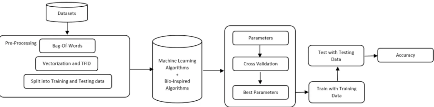
The spam detection engine should be able to take email datasets as input and with the help of text mining and opti-mized supervised algorithms, it should be able to classify the the email as ham or spam. Figure-1 represents the process that is followed to implement the model.

IV. TOOLS AND TECHNIQUES

Some of the tools and techniques used in this work are discussed below.

A. WEKA

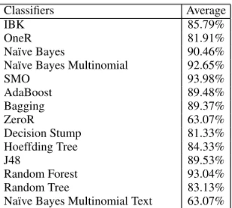
WEKA is a GUI tool that allows to load a dataset and apply different functions/rules upon an algorithm [51]. The application allows to apply the classification, regression, clustering algorithms and enable to visualise the data and the performance of the algorithm. An ’.arff’ file format of the spam datasets were fed into the program.

TABLE 1. WEKA Results

Classifiers Average

IBK 85.79%

OneR 81.91%

Naïve Bayes 90.46%

Naïve Bayes Multinomial 92.65%

SMO 93.98% AdaBoost 89.48% Bagging 89.37% ZeroR 63.07% Decision Stump 81.33% Hoeffding Tree 84.33% J48 89.53% Random Forest 93.04% Random Tree 83.13%

Naïve Bayes Multinomial Text 63.07%

Table-1 provides the average accuracy taken from the datasets for each algorithm within WEKA. The highest ac-curacy was provided by Multinomial Naïve Bayes (MNB), SMO, J48 and Random Forest. Three Naïve Bayes algo-rithms were tested using WEKA and MNB was the better amongst the three.

In this experiment WEKA acted as a black box and pro-vided the better performing algorithms which were Support Vector, Random Forest, Naïve Bayes and Decision Tree.

(6)

FIGURE 1. Spam detection block diagram

Since spam email detection falls into classification cate-gory, supervised learning method will be used. Supervised learning is a concept where the dataset is split into two parts: 1) Training data and 2) Testing data. The main aim of this learning method is to train a classifier with a given data and parameters and then predict the outcome with the testing dataset which will not be known to the program or classifier [12].

The models will be trained with a training dataset of 60%, 70%, 75% and 80%. Once the model is trained, model will be provided with the testing dataset which is distributed as 40%, 30%, 25% and 20% respectively with training dataset. This will provide a better knowledge of what percentage split is best suited and thus be more efficient to work with majority of the datasets. This will provide results on classifiers work-ing best with more or less trainwork-ing data.

B. SCIKIT-LEARN

Scikit-Learn (SKLearn) is an environment that is incorpo-rated with Python programming language. The library offers a wide range of supervised algorithms that will be suitable for this project [13]. The library offers high-level imple-mentation to train with the ’Fit’ methods and ’predict’ from an estimator (Classifier). It also offers to perform the cross validation, feature selection, feature extraction and parameter tuning [14].

C. KERAS

Keras is an API that supports Neural Networks. The API supports other deep learning algorithms for easy and fast ap-proach. It offers CPU and GPU running capabilities in order to simultaneously process the models. Online tutorials are available for neural network for learning and development. Their guide demonstrates the performance optimization tech-niques to utilize GPU and ways to work with RNN algorithm and other deep learning algorithms [15].

D. TENSORFLOW

Tensorflow is an end-to-end ML platform that is developed by Google. The architecture lets a user run the program on multiple CPUs and it also has access to GPUs. The website also provides a learning platform for both beginners and

experts. TensorFlow can also be incorporated with Keras to perform deep learning experiments [16].

E. PYTHON PLATFORMS

Research was conducted into the different platforms that could be used for ML program implementation in Python.

1) Spyder

Spyder is an Integrated Development Environment platform for Python programming language [17]. Spyder is incorpo-rated within the Anaconda framework. The software allows the user to investigate the workings of a program. The pro-gram is capable to include multiple panels such as ‘console’ where the output can be seen, ‘Variable Explorer’ where the assignment of the variables can be investigated, ‘Editor’ to edit the program and other panels such as ‘File Explorer’ and ’History’.

2) Jupyter Notebook

This is an open source tool that provides a Python framework. This is similar to ‘Spyder’ IDE, except this tool lets a user run the source code via a web browser [18]. Anaconda framework also offers ‘Jupyter’ to be utilised by the user through the local server.

F. ONLINE PLATFORMS

Along with the desktop-based platforms, other online plat-forms that offers additional support are: Google Collabora-tory and Kaggle. Both platforms are the top ML and DL based that also offers TPU (Tensor Processing Unit) [19] along with CPU and GPU. Multiple core servers can also be accessed. The platforms are cloud-based, and the user’s program is run until the ‘Runtime’ is ended.

V. MACHINE LEARNING MODELS

The subsections below explain each of the Machine Learning models that will be implemented to achieve the aim of this work. The sections are accompanied with mathematical equations along with the pseudocode algorithms. The algo-rithms define the variables "TrX" as a Training subset of "X" and "TeX" as Testing subset.

(7)

A. NAÏVE BAYES - MULTINOMIAL

Naïve Bayes model is used to resolve classification problems by using probability techniques. The Naïve Bayes algorithm for this paper can be denoted as equation-1 [20]:

P(Class|WORD) = (P(WORD|Class)×P(Class))

(P(WORD)) (1)

where WORD is (word1, word2,. . .wordn) from within an uploaded email and ‘Class’ is either ‘Spam’ or ‘Ham’. The algorithm calculates the probability of a class from the bag of words provided by the program. Where P(Class | WORD) is a posterior probability, P(WORD | Class) is likelihood and P(Class) is the prior probability [21].

If ‘Class’ = Spam, the equation could be rewritten to find the spam email from the given words, and this can be further simplified as equation-2:

P(Class|WORD) =Γ

n

i=1P(word_i|Spam)×P(Spam)

P(word_1,word_2, ...word_n) (2) There are three types of Naïve Bayes algorithms: Multi-nomial, Gaussian and Bernoulli. Multinomial Naïve Bayes algorithm has been selected to perform the spam email iden-tification because it is text related and outperforms Gaussian and Bernoulli [22] [23].

Multinomial Naïve Bayes (MNB) classifier uses Multino-mial Distribution for each given feature, focusing on term frequency. The Multinomial Naïve Bayes can be denoted as equation-3 [23]:

P(p|n)∝P(p) Y

1≤k≤nd

P(tk|p) (3)

where the number of token is represented by nd, n is the number of emails and P(tk|p) is calculated by:

P(tk|p) =

(count(tk|p) + 1)

(count(tp) +|V|)

(4)

In the equations (3) and (4),P(tk|p)is identified as the conditional probability for MNB. The tk is the spam term occurrence within an email andP(p)is classed as the prior probability. 1 and |V| are identified as the smoothing constant for the algorithm.

To test this algorithm, MNB module was loaded from the Scikit-learn library. The parameters for this model are optional. If none is specified, the default values are: Alpha value set to ‘1.0’, Fit Prior is set to ‘True’ and Class Prior is set to ‘None’ [23] [24].

The algorithm-1 shows the pseudocode for Multinomial Naïve Bayes with spam classification where "Tr" is Training and "Te" is Testing. The ˆP(tk|p)is the estimating/predicting variable, also known as the conditional probability.

Algorithm 1:Multinomial Naïve Bayes Initialise Input Variables;

N←No. of Documents; X←Datapoints; y←Target Inputs;

fori= 0; i < T rX; i+ +do if(i,y) = Spamthen

Learn i = Spam; else

Learn i = Ham;

fort in testSize// Test sizes = 20, 25, 30 and 40

do

forK in CVdo

X_test and y_test= testing size; X_train and y_train= training size; fori= 0; i < T eX; i+ +do

Calculate ˆP(tk|p); Calculate the Accuracy; returntk;

B. SUPPORT VECTOR MACHINE

This algorithm plots each node from a dataset within a dimensional plane and through classification technique the cluster of data is separated by a hyperplane into their re-spective groups [25]. The hyperplane can be described as equation-5:

H =V X+c (5)

where c is a constant andV is the vector. The SGD Clas-sifier was loaded from scikit-learn library, which is the lin-ear model with ‘Stochastic Gradient Descent (SGD)’, also known as the optimized version of SVM. This algorithm provides more accurate results than SVM (SVC algorithm) itself. Disadvantage of working with SVC algorithm is that it cannot handle a large dataset, whereas SGD provides efficiency and other tuning opportunities.

The algorithm-2 shows the pseudocode for Stochastic Gra-dient Descent.

The model was implemented with ‘Alpha’, ‘Epsilon’ and ‘Tol’ values with default as ‘Hinge’ for loss providing linear SVM, also known as ’Soft-Margin’ which is easier to com-pute [25].

The algorithm uses the learning rate to iterate over the sample data to optimize the Linear algorithm and it is denoted by the following equation-6 for the default learning rate as ’Optimal’:

1

α(t0+t) (6)

where t is the time step which is acquired by multiplying number of iterations with number of samples (Emails). The Learning Rate allows implementation of the parameter space

(8)

Algorithm 2:Stochastic Gradient Descent Initialise Input Variables;

N←No. of Documents; X←Datapoints; y←Target Inputs;

Initialise Alpha, Epsilon values; fori= 0; i < T eX; i+ +do

Calculate Hyperplane// Equation (5)

Measure the Distance (Xi,Xj);

fort in testSize// Test sizes= 20, 25, 30 and 40

do

forK in CVdo

X_test and y_test= testing size; X_train and y_train= training size; Call the SGD function;

Calculate the Training Error; Calculate the Rate;

Calculate the Accuracy; returntk;

during the training time. Theαis represents the regulariza-tion term andt0is a hueristic approach.

C. DECISION TREE CLASSIFIER

The Decision Tree model is based on the predictive method. The model creates a category which is further distributed into sub-categories and so on. The algorithm runs until the user has terminated or the program has reached its end decision. The model predicts the value of the data by learning from the provided training data. The longer and deeper the tree implies it has more complicated rules to be executed.

The algorithm-3 shows the pseudo-code for Decision Tree, where it terminates at the end of the node for each split of the tree depth.

Similar to MNB and SGD, Decision Tree (DT) algorithm was loaded from the Scikit-learn library and it is executed on the default parameters which are ‘Gini’ for Criterion and ‘best’ for Splitter. The advantage of Gini is that it calculates the incorrectly labelled data that was selected randomly [26]. This is given by the below equation-7:

Gini :Gi= 1− n

X

k=1

p(i,k)2 (7)

The second criterion is ‘entropy’ which is based on in-formation gain based on the selected attributes and it is calculated by equation-8 [26]: . Entropy :Hi= n X k=1 pik6=0

p(i,k)log2(p(i,k)) (8)

whereP is the probability andiis a node from the training data within both equation (7) and (8).

Algorithm 3:Decision Tree - CART Algorithm Initialise Input Variables;

N←No. of Documents; X←Datapoints; y←Target Inputs; Ln = Number of Leaves; D = Tree Depth ; C = Criterion// (Gi) or (Hi)

do

forK in CVdo

X_test and y_test= testing size; X_train and y_train= training size; fori < Xdo

Call DT function; forj < Ddo

Calculate the best split; Predict the class (c); Ln++;

For the node: (c,C)// Use equation (7) or (8)

returnPredicted Class (ˆc) Calculate the Accuracy;

D. RANDOM FOREST CLASSIFIER

Random Forest (RF) algorithm can be used for both classi-fication and regression. The algorithm predicts the classes by using multiple decision tree, where each tree predicts the classification class. This is evaluated by the RF model to select the high number of predicted class as an assigned prediction [27].

The algorithm-4 explains the workings of the Random Forest classifier with the Spam Email dataset, where Fˆc is the outcome predicted from the entire forest.

Equation-7 and equation-8 are also utilised to calculate the Gini and Entropy for Random Forest (RF) algorithm to calculate the Criterion.

This module was loaded from Scikit-learn library and it is based on the depth of the tree and number of DT to be produced. These are usually considered as the termination criteria. This means the more the depth and the number of trees the more the computational time required for the algorithm.

E. MULTI-LAYER PERCEPTRON (MLP)

The MLP is a feed-forward Artificial Neural Network (ANN). It is a supervised method which includes non-linear hidden layers between the input and the output layer. The algorithm works with the linear activation function on a training dataset set by default known as Hyperbolic Tan (equation-9) [28]:

(9)

Algorithm 4:Random Forest Initialise Input Variables; N←No. of Documents; X←Datapoints; y←Target Inputs; Ln = Number of Leaves; D = Tree Depth ; C = Criterion// (Gi) or (Hi) Nt = Number of Trees;

do

forK in CVdo

X_test and y_test= testing size; X_train and y_train= training size; fori < Ntdo

fori < Ddo

Randomly select from X; Split the nodes with C;

Calculate the Predicted ˆc from each tree;

returnPredicted from the tree Tˆc Provide the array of DT decision for all

trees;

Calculate the prediction from the majority; returnPredicted from the Forest Fˆc

wheremis the input (spam words in this case) andois the number of outputs from the function. The algorithm can have one or more layers between input and output layer known as ‘Hidden Layer(s)’. The hidden layer accepts the values from the previous layer and transforms with linear summation, whereas the ‘Output’ layer provides the output values after transformation from the previous hidden layer [28].

The algorithm-5 shows the pseudocode for Multi-Layer Perceptron.

The algorithm uses back-propagation technique to cal-culate the gradient descent for each variable weight. The algorithm has the ability to learn when it becomes part of one neuron and one hidden layer of MLP function as indicated in equation-10.

f(x) =W2g(W1Tx+b1) +b2 (10)

where W2 and W1 are the weights from the input layer

and hidden layer. The W1

i becomes the part of ni layers in the hidden layer [28]. To compare the results of NN and ML models, the modules were loaded from the Scikit-learn similar to the ML models. The default parameter was changed for hidden layer to lower number of neurons for faster computation.

Algorithm 5:Multi-Layer Perceptron Initialise Input Variables;

N←No. of Documents; X←Datapoints; y←Target Inputs; H = No.Hidden Layer; Nu = No.of Neurons; Ac= Activation; S = Solver;

do

forK in CVdo

X_test and y_test= testing size; X_train and y_train= training size; Call the MLP Function←H, Nu, Solver ; Calculate the Error Rate;

Error×Activation; Calculate the Accuracy;

VI. PROGRAM STRUCTURE, DATASETS AND REQUIREMENTS

The Python program will load all the necessary Python libraries that will assist the ML modules to classify the emails and detect the spam emails.

A. ADDING CORPUS

This section will load all the email datasets within the program and distribute into training and testing data. This process will be accepting the datasets in ’*.txt’ format for individual email (Ham and Spam). This is to help understand the real-world issues and how can they be tackled.

B. TOKENIZATION

Tokenization is the method where the sentences within an email are broken into individual words (tokens). These tokens are saved into an array and used towards the testing data to identify the occurrence of every word in an email. This will help the algorithms in predicting whether the email should be considered as spam or ham [49].

C. FEATURE EXTRACTION AND STOP WORDS

This was used to remove the unnecessary words and char-acters within each email, and creates a bag of words for the algorithms to compare against.

The module ‘Count Vectorizer’ from Scikit-learn assigns numbers to each word/token while counting and provides its occurrence within an email. The instance is invoked to exclude the English stopwords, and these are the words such as: A, In, The, Are, As, Is etc., as they are not very useful to classify whether the email is spam or not. This instance is then fitted for the program to learn the vocabulary [49].

Once tokenized, the program applies ‘TfidfTransformer’ module to compute the Inverse Document Frequency (IDF).

(10)

The most occurring words within the documents will be assigned values between 0-1, and lower the value of the word means that they are not unique. This allows the algorithms/-modules to read the data [49]. The TF-IDF can be calculated by the Equation-11 where (t, d) is the term frequency (t) within a document (d):

tf−idf(t,d) = tf(t,d)×idf(t) (11) where IDF is calculated by the Equation-12, given nis the number of documents:

idf(t) = log( n

idf(t)) + 1 (12)

D. MODEL TRAINING AND TESTING PHASE

As discussed through the research, supervised learning meth-ods were used and the model was trained with known data and tested with unknown data to predict the accuracy and other performance measures. To acquire the reliable results K-Fold cross validation was applied. This method does have its disadvantages such as, there is a chance that the testing data could be all spam emails, or the training set could include the majority of spam emails. This was resolved by Stratified K-fold cross validation, which separates the data while making sure to have a good range of Spam and Ham into the distributed set [50].

Lastly, parameter tuning was conducted with the Scikit-Learn and bio-inspired algorithms approach to try and im-prove the accuracy of ML models. This provides a platform to compare the Scikit-learn library with the bio-inspired algorithms

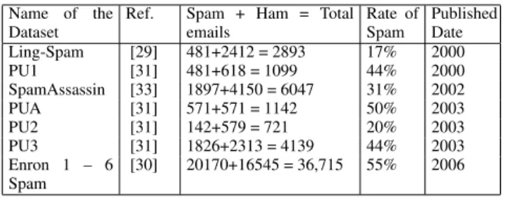
E. DATASETS

The project accessed the publicly available datasets and included each email as an individual text file. The text files were string based. A list of the few spam email datasets from the public repository are explained below:

1) Ling-Spam dataset is divided into 10 parts from the ‘bare’ distribution that includes individual emails as a text file (.txt). This data is not pre-processed, and it includes numbers, alphabets and characters [29]. Each part was trained and tested to acquire the average accuracy.

2) Enron dataset includes 6 separate datasets that contain 3000-4000 individual emails as text files. The dataset includes numbers, alphabets and characters [30]. 3) The PUA dataset is a numerical dataset that includes

sets/combination of numbers characterised as a string. PU1, PU2 and PU3 are similar to PUA dataset but include different weights of spam and ham emails and they are extracted from different users [31]. Folders include individual emails as a text file. For all PU datasets, the publisher has replaced the tokens with a unique combination of numbers to respect their user’s privacy. The respective words for these unique num-bers have not been made public, making the process of removing certain features difficult [32].

From PU1 and PU2 datasets, duplicate emails that were received were discarded manually. Whereas in PU3 and PUA, this was conducted with the UNIX command ’diff’. Each of these emails were collected during different lengths of time for both Ham and Spam emails.

4) SpamAssassin dataset is more advanced with header information such as source or From address, IP ad-dress, return path, message ID and delivery informa-tion. Each individual email within the folder will be converted into text files [33].

Table-2 presents the spam rate of each of the datasets that are used within this project along with their published date [2].

TABLE 2. Datasets

Name of the Dataset

Ref. Spam + Ham = Total emails Rate of Spam Published Date Ling-Spam [29] 481+2412 = 2893 17% 2000 PU1 [31] 481+618 = 1099 44% 2000 SpamAssassin [33] 1897+4150 = 6047 31% 2002 PUA [31] 571+571 = 1142 50% 2003 PU2 [31] 142+579 = 721 20% 2003 PU3 [31] 1826+2313 = 4139 44% 2003 Enron 1 – 6 Spam [30] 20170+16545 = 36,715 55% 2006

F. SOFTWARE AND HARDWARE

Python 3.4 or above was used and Anaconda platform seemed like a good option as it provides the advantage of using both Spyder and Jupyter Notebook for implementing the programs.

Some online applications such as Google Collaboratory and Kaggle can be used to speed up the training and testing process for the multiple datasets. This can be helpful towards any NN algorithms that can be implemented.

The project was conducted on a standard laptop, with 8 GB RAM and AMD Ryzen 3 3200U (2.60 GHz) processor.

G. LIBRARIES AND MODULES

Scikit-Learn will be used as it offers the majority of the machine learning libraries and dataset processing modules.

As per the papers discussed in the related work section, PSO performed much better among the bio-inspired algo-rithms. For comparison purposes, the second implementation of bio-inspired algorithm will be based on human evolution. Libraries like PySwarms for Particle Swarm Optimisation and TPOT for Genetic Algorithm will be utilised to optimise the accuracy of the machine learning algorithms.

VII. PERFORMANCE MEASURES

There are different performance metrics that were used in this work as follows.

A. CONFUSION MATRIX

The detection of spam emails can be evaluated by different performance measures. Confusion Matrix is being used to

(11)

visualise the detection of the emails for models. Confusion matrix can be defined as below:

HAM SPAM

HAM TN FP

SPAM FN TP

where [34]:

1) TN = True Negative – Ham email predicted as ham 2) TP = True Positive – Spam email predicted as spam 3) FP = False Positive – Spam email predicted as ham 4) FN = False Negative – Ham email predicted as spam B. ACCURACY

The research was aimed at finding the highest accuracy for detecting the emails correctly as ham and spam. The module from the Scikit-learn library called ‘Accuracy’ helped anal-yse the correct number of emails classified as ‘Spam’ and ‘Ham’. This can be measured by equation-13 below [35]:

Accuracy = (TN + TP)

(TP + FN + FP + TN) (13) where the denominator of the equation is the total number of emails within the testing data.

C. RECALL

The recall measurement provides the calculation of how many emails were correctly predicted as spam from the total number of spam emails that were provided. This is defined by equation-14, where ‘TP + FN’ are the total number of spam emails within the testing data [35]:

Recall = TP

TP + FN (14)

D. PRECISION

The precision measurement is to calculate the correctly iden-tified values, meaning how many correctly ideniden-tified spam emails have been classified from the given set of positive emails. This means to calculate the total number of emails which were correctly predicted as positive from amongst the total number of emails predicted positive [35]. This is defined by equation-15:

Precision = TP

TP + FP (15)

E. F1-SCORE

The F-measure or the value ofFβis calculated with the help of precision and recall scores, where β is identified as 1,

Fβ orF1 provides the F1-score. F1-score is the ‘Harmonic

mean’ of the precision and recall values. This can be defined by equation-16 [35]:

Fβ=

(1 +β2_)(precision_×_recall)

(β2_×_{(precision + recall))} (16)

when the β is substituted with the value 1, the formula is simplified to:

Fβ=

2×(precision×recall)

(1×precision + recall) (17)

VIII. RESULTS OF BASE MODEL ON DATASETS

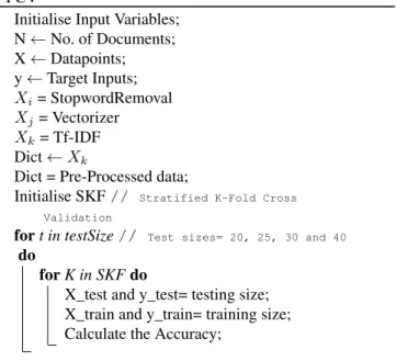
Stratified K-Fold Cross Validation (SKFCV) was applied to all the machine learning models. Algorithm-6 represents the pseudocode for the base models, this was executed with the default values for parameters explained in section V and VI.

Algorithm 6:Base Model Implementation with SK-FCV

Initialise Input Variables; N←No. of Documents; X←Datapoints; y←Target Inputs; Xi= StopwordRemoval Xj= Vectorizer Xk= Tf-IDF Dict←Xk

Dict = Pre-Processed data;

Initialise SKF// Stratified K-Fold Cross Validation

do

forK in SKFdo

X_test and y_test= testing size; X_train and y_train= training size; Calculate the Accuracy;

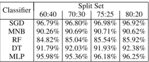
The visual representation of five models is shown in Figure-2: ML algorithms, from left: SGD, MNB, RF, DT and MLP. The figure displays the 4 split sets used for each classifier (CLF). The selected algorithms have provided 90% and above accuracy for email detection except RF. This was applied on the 7 datasets and the average was taken. Amongst the five algorithm RF has performed poorly and SGD is the highest performing algorithm.

(12)

The respective accuracies for each split set in Figure-2 are defined in Table-3.

TABLE 3. Stratified K-Fold Cross-Validation - Accuracy

Classifier _60:40 _70:30Split Set_75:25 _80:20 SGD 96.79% 96.80% 96.98% 96.92% MNB 90.26% 90.69% 90.71% 90.62% RF 84.82% 85.04% 85.54% 85.92% DT 91.79% 92.03% 91.93% 92.38% MLP 95.98% 95.36% 96.18% 96.25%

Computational timing depends on the depth of a dataset and the classification. For base classifiers, the approximate times are shown below to train for each iteration of cross-validation for the respective classifiers.

1) Naïve Bayes: 0.003 sec to 0.0013 sec approx. 2) Support Vector Machine: 0.040 sec approx. 3) Random Forest: 1.080 sec approx.

4) Decision Tree: 4.06 sec approx. 5) Multi-Layer Perceptron: 8.0 sec approx.

The experiment evaluates that the more the training data, the better accuracy the testing data provides. The NN model will later be tested for 75:25 and 80:20 split set with bio-inspired algorithms.

IX. TUNING OF PARAMETERS

For every model, certain parameters were selected and pro-vided with a range of possibilities. These parameters are the ones that have high impact towards detecting the emails and learning rate. This will then be implemented within bio-inspired algorithms.

A. SGD PARAMETERS

Hyperparameter tuning the algorithm offers 3 parameters from the SGD algorithm: Alpha values, Epsilon values and Tol values for the search space. Values for all three keys ranged from 0.0001 to 1000 as a dictionary.

• Alpha: The variable could help set the optimal learning rate. It is also classed as the constant for regularization term.

• Epsilon: This value determines the learning rate for the algorithm.

• Tol: This is the criteria for termination. B. MNB PARAMETERS

The dictionary of parameters provided for the optimization were values of:

• Alpha: This is used as a smoothing parameter for Laplace or Lidstone to the raw counts. This parameter will be passed as a float for PSO. This is combined with the number of features within the module. The value ranged from 0.0001 to 1000 as a dictionary

• Fit Prior: This is to learn the class probabilities.

C. RF PARAMETERS

• Number of estimators: This states number of trees in the forest.

• Max depth: This indicated maximum depth of the tree.

• Minimum leaf sample: Specifies the minimum number of leaves at the leaf node.

• Criterion: This is in a string format. This is a tree

specific parameter that can be ‘Gini’ for Gini impurity or ‘Entropy’ for information gain.

D. DT PARAMETERS

• Splitter: This is a string-based parameter which can be

either ‘Best’ or ‘Random’. This specifies the strategy for the split at a node.

• Max Depth: This will specify the depth of the tree. • Criterion: This measures the quality of the split. • Minimum leaf sample: This is passed as an integer

to specify the minimum number of samples that are necessary at the leaf node.

E. MLP PARAMETERS

• Hidden layer sizes: Number of neurons to be considered by the classifier. This is where each feature is intercon-nected with each neuron.

• Alpha: This is a regularization parameter. The value was ranged from 0.001 to 0.01. These values were less than the default value.

• Solver: According to the Scikit-learn documentation, the solver when set to ‘LBFGS’, the module’s perfor-mance and speed can increase on small datasets. Due to the computational time required for the MLP classifier, for this project purpose, the optimisation was done on ’5’ hidden layers and the solver set to ‘LBFGS’ which is an optimizer that can converge fast and provide better performance. The greater number of neurons added to the hidden layer, the more time it will require to train the model [28].

X. BIO-INSPIRED OPTIMIZATION ALGORITHMS

There are two bio-inspired optimization approaches that are discussed here which helped to improve the results of the experiments, i.e. Particle Swarm Optimisation and Genetic Algorithm.

A. PARTICLE SWARM OPTIMISATION

The PSO is based on the swarming methods observed in fish or birds. The particles are evaluated based on their best position and overall global position. Particles within a search space are scattered to find the global best position.

(13)

The Pyswarms library offers different calculations and techniques for PSO to be used with an ML model such as feature subset selection or parameter tuning optimization. As researched in the previous sections, the feature selection can reduce feature space but can also discard some features that can be useful during the classification. Therefore, PSO will be used to tune and find the hyper-parameter for a given ML/NN model.

The PSO will use the ‘GlobalBestPSO’ from the

‘pyswarms.single.global_best’ module. This will

then use the ‘optimize’ method with an objective function and number of iterations to run the PSO before terminating. This will then provide the ‘Global best cost’ and ‘Global Best position” [36].

The ‘global_best’ module and equation-18 denotes the updating of each particle position:

xi(t+ 1) =xi(t) +vi(t+ 1) (18) where xi is the position of the particle, t is the current timestamp and t + 1 is the computed velocity which gets updated. The velocity (vi) can be further defined as below:

vij(t+ 1) =w×vij(t) +c1r1j(t)[yij(t) −xij(t)] +c2r2j(t)[ˆyj(t)−xij(t)]

(19) wherer1andr2are the random numbers,c1is the cognitive parameter and c2 is the social parameter. These parameters control the behaviours of the particle. The w is the inertia parameter that controls the swarm’s movements, which is the important parameter and hence the value is bigger than the other parameters. The parameters for cognitive and inertia parameter remained with default value as the demonstrated algorithm in ‘Optimizer’ package [36].

The social parameter was increased by 0.5. The parameters passed onto theGlobal_bestmodule are:

• Number of particles: 10; this was considered by the examples set within the Pyswarms library.

• Dimension: This is the number of dimensions within a given space. The number of parameters for the base algorithms such as Alpha, Tol, Epsilon etc.

• Options: C1 = 0.5, C2 = 0.7 and W = 0.9. These

parameters have effect on the computation time.

• Bounds: This is a tuple, obtained through the dimension.

Higher and lower value within the base algorithm’s parameters will be considered.

The option setting of coefficients is important. The smaller the number, the distance of the particle movement will be small too. This can take more time in computing the models. Algorithm-7 shows the pseudocode for Particle Swarm Optimization. This is implemented on top of the base model in algorithm-6.

Figure-3 shows the visual representation of PSO algorithm accuracies for the 5 models/classifiers. The accuracy score was taken from the average of all seven datasets. The highest accuracy of 98.47% was provided by Naïve Bayes on 80%

Algorithm 7:PSO Implementation Initialise Input Variables;

N←No. of Documents; X←Datapoints; y←Target Inputs; Xi= StopwordRemoval; Xj= Vectorizer; Xk= Tf-IDF; Dict←Xkl

Initialise ML Parameters;// This will include the key and the values

Declare ML Algorithm;// MNB, SGD, DT, RF and MLP

DefPSO:

Initialise PSO parameters; C1=0.5;// Cognitive Parameter

C2=0.7;// Social Parameter

W=0.9;// Weight Ni=NumberOfIteration;

Np=NumberOfParticles; Calculating the Dimension;

(Key,Value)←Parameters;// The parameters of the algorithm i.e MNB, SGD

Call PSO G_Best algorithm;// Global Best

PSO Module←Dimension, C1, C2, w,Ni, Np; Call Objective FunctionOf;

PSO←Of;

Calculate the Best_Position of the Swarm; Best_Position←Ni;

Calculate the Measures;

Measures←Best_position, TrData, TeData; returnAccuracy

DefOf:

fori <Npdo

Initialise StratifiedKF; Calculate the Score;

returnThe array of accuraciesAq

// conducted with the dimensions and the Key and Value provided

fort in test sizedo

X_test and y_test= testing size; X_train and y_train= training size; Call the function PSO (training and testing

(14)

training data and 20% testing data. Overall, MNB provided higher accuracy from all the other classifiers.

FIGURE 3. Particle Swarm Optimization – Accuracy

The respective accuracies for each split set in the above figure-3 are defined in Table-4.

TABLE 4. PSO - Accuracy

Classifier Split Set

60:40 70:30 75:25 80:20 SGD 97.37% 97.54% 97.21% 97.64% MNB 98.41% 98.38% 98.43% 98.47% RF 91.94% 91.37% 91.62% 90.81% DT 91.37% 91.65% 92.29% 92.28% MLP - - 97.11% 97.18%

The entire program took nearly a day for all 5 classifiers to run on different platforms. The computational time required for the runs depending on the dataset are as follows:

1) Multinominal Naïve Bayes: 5 mins approx. 2) Support Vector Machine: 5 mins approx. 3) Random Forest: 2 mins to 15 mins approx. 4) Decision Tree: 2 mins to 25 mins approx. 5) Multi-Layer Perceptron: 25 min to 1hour approx. In terms of datasets, the highest achieving algorithm is MNB with 70:30 split set on SpamAssassin dataset. The parameters chosen were: Alpha: ‘0.0004940843999793119’ and Fit Prior: ’false’.

The highest occurred accuracy from the given datasets along with the classifier (CLF), Test Size and the parameters that were selected by the PSO algorithm is shown in table-5. Tables 6, 7, 8 and 9, represent the F1-score, Precision and Recall in comparison to Accuracy. It shows the average of performance measurements for the ML algorithms applied on 7 datasets. The MNB algorithm was the one which provided the best performance amongst other ML algorithms for all four different split sets. The percentage calculated are taken from the average of all 7 datasets.

From these tables, 98% of the emails were correctly de-tected by MNB on the average. The average precision was 97.50% and average recall was 97.40% and average F1-score was 97.50%.

TABLE 5. PSO Selected Values

CLF Dataset Test

Size

Acc. Parameters MNB SpamAssassin 70:30 99.89% Alpha:

0.0004940843999793119, Fit Prior: false

SGD SpamAssassin 80:20 99.67% Alpha:

0.00011028738827772605, Epsilon:

0.0008410556148690041, Tol: 0.0004946026859321408 RF SpamAssassin 60:40 97.75% No. of estimators: 5, Max

Depth: 7.154304302293813, Min leaf sample: 1, Criterion: ’entropy’

DT SpamAssassin 80:20 99.33% Splitter: ’best’, Criterion: ’entropy’, Max Depth: 6.910921197436718, Min Leaf Sample: 2

MLP SpamAssassin 80:20 99.67% Hidden Layer Size: (5,), Al-pha: 0.005177077568305584, Solver: ’lbfgs’

TABLE 6. PSO 60:40 Split Set

Classifier Accuracy F1-score Precision Recall

SGD 97.37% 95.37% 97.18% 93.83%

MNB 98.41% 97.80% 97.55% 97.55%

RF 91.94% 79.57% 94.23% 74.76%

DT 91.37% 85.16% 88.10% 83.24%

SGD 97.54% 96.21% 97.24% 95.20%

MNB 98.38% 97.51% 97.82% 97.31%

RF 91.37% 77.67% 96.95% 70.36%

DT 91.65% 86.64% 87.81% 85.96%

SGD 97.21% 94.79% 97.11% 93.11%

MNB 98.43% 97.60% 97.73% 97.24%

RF 91.62% 77.88% 96.58% 92.51%

DT 92.29% 87.48% 88.27% 88.04%

SGD 97.64% 95.78% 96.80% 95.59%

MNB 98.47% 97.54% 97.23% 97.86%

RF 90.81% 74.79% 96.11% 66.49%

DT 92.28% 86.71% 88.07% 86.45%

The highest accuracy noted was 98.47% achieved by MNB, providing precision of 97.23%, recall of 97.86% and F1-Score of 97.54%. This was achieved with training size 80% and Testing size 20%.

(15)

B. GENETIC ALGORITHM

The GA algorithm is an evolutionary algorithm based on Darwinian natural selection that selects the fittest individual from the given population. This involves the principle of variation, inheritance and selection. The algorithm maintains a population size and the individuals have a unique number (Chromosomes) that are binary represented. The algorithm iterates through a fitness function where best individuals are selected for reproduction of the offspring. The higher the fitness, the higher the probability [8].

Implementation of the GA was conducted with the help of TPOT library. The program selects the best parameters from a given dictionary of parameters. The TPOT classifier is then trained with cross validation. The parameters given to the TPOT are as follows [37]:

• Generation: Number of times the pipeline will conduct the optimization process. The default value is 100. The program has set this parameter as ‘10’.

• Population size: Number of individuals participating for Genetic programming within each generation. Default is 100. The program has set this parameter as ‘40’

• Offspring size: Offspring to be produced in each genera-tion. Default is 100. The program has set this parameter as ‘20’.

The program runs for 10 generations with 40 population size and 20 offspring production. This means 400 (10 x 40) hyperparameter combinations will be evaluated before termi-nating for each generation. Each pipeline will be evaluated with 10-fold cross validation i.e. 400 x 10. Once the TPOT classifier is terminated, it provides the best pipeline param-eters. The entire pipeline will be evaluated [(Generation x lambda) + Population size] = 240 times, where lambda is Offspring size. If no Offspring size is provided the pipeline will evaluate by substituting population as ‘lambda’.

The mutation rate and the crossover rate were set as default. The mutation rate is 0.9, which is the changes in the parameter value. The crossover rate is 0.1, which is the percentage of the individuals required from the population to create offspring. The TPOT warns that ‘Mutation rate + crossover rate’ should not exceed 1.0.

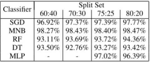
Algorithm-8 shows the pseudocode for Genetic Algorithm. This is implemented on top of the base model in algorithm-6. The Figure-4 shows the visual representation of GA algo-rithm accuracies for the 5 classifiers.

The respective accuracies for each split set in the figure-4 are defined in Table-10.

The computational time required for the runs depending on the dataset is given as:

1) Mutinomial Naïve Bayes: 12 mins approx. 2) Support Vector Machine: 15 mins approx. 3) Random Forest: 3 mins to 20 mins approx. 4) Decision Tree: 15 mins to 40 mins approx. 5) Multi-Layer Perceptron: 1 hour to 2 hours approx. Table-11 shows the output for every classifier that achieved highest accuracy, which is similar to that conducted with

Algorithm 8:GA Implementation Initialise Input Variables; N←No. of Documents; X←Datapoints; y←Target Inputs; Xi= StopwordRemoval; Xj= Vectorizer; Xk= Tf-IDF; Dict←Xk;

Initialise ML Parameters;// This will include the key and the values

Declare ML Algorithm;// MNB, SGD, DT, RF and MLP

DefGA: Initialise GA parameters; G = GenerationSize; P = PopulationSize; Os=OffSpringSize; M = MutationRate; C = CrossoverRate;

K = StratifiedKF;// Cross Validation

GA(TPOT) Module←G, P,Os, M, C; Calculate the Survivor of the Swarm; forG in Generationdo

forP in Populationdo fori < Kdo

Survival←Calculate the Fitness; Select two Individual;

Produce OffSpring←Os; Mutate←OffSpring, M; returnKScore

Calculate Parameters; returnP arameters

Calculate the Measures;

Measures←Parameters, TrData, TeData; returnAccuracy

fort in test sizedo

X_test and y_test= testing size; X_train and y_train= training size;

Call the function GA (training and testing data);

TABLE 10. GA - Accuracy

Classifier Split Set

60:40 70:30 75:25 80:20 SGD 96.92% 97.37% 97.39% 97.77% MNB 98.27% 98.43% 98.40% 98.47% RF 93.11% 93.69% 93.72% 94.36% DT 93.50% 92.76% 93.27% 93.42% MLP - - 97.02% 96.39%

PSO. The highest achieving accuracy of 100% was by MNB on 80:20 split set with SpamAssassin dataset. The parameters chosen were: Alpha: 0.01, Fit Prior: ’false’.

(16)

FIGURE 4. Genetic Algorithm – Accuracy TABLE 11. GA Selected Values

CLF Dataset Test

Size

Acc. Parameters

MNB SpamAssassin 80:20 100% Alpha: 0.01, Fit Prior: ’false’ SGD SpamAssassin 80:20 99.83% Alpha: 0.0001, Epsilon: 1.0,

Tol: 0.1

RF SpamAssassin 75:25 98.54% Criterion: ’entropy’, Max Depth: 30, Min Leaf Sample: 1, No. of estimators: 25 DT SpamAssassin 80:20 99.33% Criterion: ’entropy’, Max

Depth: 15, Min Leaf Sample: 1, Splitter: ’best’.

MLP SpamAssassin 75:25 and 80:20

99.33% Alpha: 0.001, Solver: ’lbfgs’.

and Recall in comparison to Accuracy when the Genetic Algorithm (GA) is applied on the machine learning (ML) algorithms. It shows the performance measurements for the ML algorithms. The MNB algorithm was the one to provides the best performance amongst other ML algorithms for all four different split sets like it did with PSO. The percentages shown are calculated from the average of all 7 datasets. TABLE 12. GA 60:40 Split Set

SGD 96.92% 95.27% 96.59% 94.13%

MNB 98.27% 97.32% 97.38% 84.63%

RF 93.11% 83.13% 96.51% 77.16%

DT 93.50% 88.42% 90.02% 86.96%

TABLE 13. GA 70:30 Split Set

SGD 97.37% 95.61% 96.98% 94.52%

MNB 98.43% 97.64% 97.76% 97.61%

RF 93.69% 85.83% 97.00% 80.11%

DT 92.76% 88.25% 89.34% 87.48%

SGD 97.39% 95.68% 97.48% 94.03%

MNB 98.40% 97.57% 98.09% 97.11%

RF 93.72% 85.73% 97.25% 80.43%

DT 93.27% 88.72% 90.68% 87.55%

SGD 97.77% 96.71% 97.61% 95.97%

MNB 98.47% 97.67% 98.01% 97.59%

RF 94.36% 87.42% 97.79% 81.74%

DT 93.42% 89.54% 91.07% 88.51%

From these tables, 98% of the emails were correctly de-tected by MNB on the average. The average precision was 97.50%, average recall was 93.00% and average F1-score was 97.00%.

The highest accuracy was 98.47% achieved by MNB, providing precision of 97.79%, recall of 81.74%, and F1-Score of 87.42%. This was achieved with training size 80% and Testing size 20%.

XI. RESULTS OF OPTIMIZED CLASSIFIERS ON DATASETS

There are two types of spam email dataset being used for this project, alphabetic-based and numeric-based files. These are described in table-16.

TABLE 16. Dataset Type

Sr.No Alphabetical Based Numerical Based

1) Ling-Spam PU1

2) Enron Spam PU2

3) SpamAssassin PU3

4) - PUA

FIGURE 5. Stochastic Gradient Descent Alpha/Num comparison Each of the four machine learning models/classifiers were tested with the average taken from the alphabetical datasets and compared with the average taken from the numerical datasets.

(17)

Figure-5 shows the split between the two types of dataset, namely numerical and alphabetical. The algorithm SGD provided the highest accuracy for alphabet-based datasets. Even though the accuracies for the numerical datasets are low, the improvement is much better than the base algorithm compared to the alphabet-based dataset.

FIGURE 6. Multinomial Naïve Bayes Alpha/Num comparison Figure-6 shows the performance of the MNB algorithm with both type of datasets. The algorithm performed similarly to SGD. The accuracy is higher for the alphabet-based dataset than the numerical dataset.

Both MNB and SGD algorithms worked well for numeri-cal and alphabet-based datasets with PSO and GA optimiza-tion. The accuracy is higher on the alphabet-based datasets for both algorithms. Split set 75:25 and 80:20 have worked better than the split set 60:40 and 70:30.

FIGURE 7. Random Forest Alpha/Num comparison

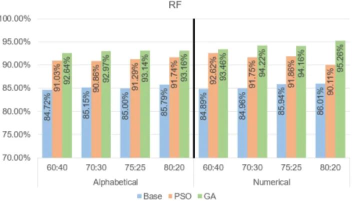
Figure-7 shows the performance of RF algorithm between the numerical and alphabetical datasets. This tree-based algo-rithm seems to have worked well with the numerical datasets in terms of accuracy and improvement.

Figure-8 shows the performance of DT algorithm. Similar to RF, the DT has worked better with numerical in terms of improvement. Whereas for alphabetical, there is very less improvement but higher accuracy.

FIGURE 8. Decision Tree Alpha/Num comparison

The tree-based algorithms (Figure-7 and Figure-8) have performed better with GA optimization than the PSO on both type of datasets.

For Neural Networks, the implementation with the PSO algorithm took more than 7 hours for 5/25 iterations to be completed for one split set with 100 neurons. Since the MLP classifier was taking more power, the algorithm was distributed between three platforms 1) Kaggle, 2) Google Collaboratory and 3) standard PC. The number of neurons were reduced to ‘50’ to acquire an idea of timing for the run. This time the algorithm took about a minimum of 6 hours to complete one split set. Hence, at the end the classifier was run with 5 Neurons providing some improvement and quicker completion.

FIGURE 9. Multi-Layer Perceptron Alpha/Num comparison The MLP classifier was experimented with the optimiza-tion techniques by integrating with PSO and GA. The classi-fier was testing with 75:25 and 80:20 split sets, as these were the highest providing accuracies for ML models/classifiers. The alphabet-based dataset performed much better than the Numerical dataset as shown in Figure-9.

XII. EVALUATION AND COMPARISON

The evaluation and performance comparison on the work is discussed in this section.

(18)

A. SPLIT SETS

Evaluating all the split sets for training and testing data on all seven datasets, sizes 72:25 and 80:20 were the top two splits to provide better accuracy and showed improvement. This could vary on the dataset size and the information separated during the split. This proves that the higher the rate of training data than testing data, better the performance achieved. This is a good sign, since when considered as a real-world example, the models will have bigger weight for training data than testing.

B. EXPERIMENTAL RESULTS - ACCURACY

According to the experiments, PSO and GA have improved the accuracy of all five models. The Multinomial Naïve Bayes (MNB) is the algorithm that has performed better than all the other algorithms. Comparing across the different types of datasets, Enron, SpamAssassin and Ling-Spam dataset provided more depth by eliminating certain features through the emails, hence, allowing the optimization techniques more search space. But the numerical dataset (PU1, PU2, PU3 and PUA) were very restricted, even though they successfully provided accuracy improvements on some split sets.

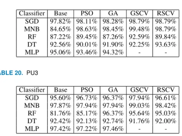
Taking the individual datasets into account, the SpamAs-sassin dataset performed very well with Naïve Bayes and Genetic Algorithm. Table-17 shows the accuracy comparison for SpamAssassin dataset on Machine Learning models for 80:20 split set. The table also compares with the optimization models that is provided by the Scikit-learn library. Grid Search CV (GSCV) and Random Search CV (RSCV) were both implemented within the base model and were loaded from the Scikit-learn library.

TABLE 17. SpamAssassin Dataset

Classifier Base PSO GA GSCV RSCV

SGD 99.28% 99.67% 99.83% 99.50% 99.66% MNB 89.28% 99.83% 100.00% 99.66% 99.66% RF 89.25% 97.33% 98.17% 98.33% 96.17% DT 98.47% 99.33% 99.33% 98.83% 99.00%

MLP 99.35% 99.67% 99.33% -

-In comparison to alphabetical datasets and numerical datasets, the tables 18, 19 and 20 show the accuracy achieved for 80:20 split set.

Taking Enron Spam dataset into account, it was the second-best corpus to work with followed by Ling-Spam. TABLE 18. Enron Spam Dataset

SGD 99.12% 99.20% 99.21% 99.17% 99.14% MNB 93.26% 98.58% 98.60% 99.52% 98.52% RF 80.88% 88.45% 94.05% 94.76% 94.27% DT 96.05% 93.62% 96.07% 95.50% 94.93%

MLP 98.12% 99.18% 99.05% -

-An average of all four PU datasets were taken into con-sideration and PU3 dataset provided better results and the highest accuracy amongst all four and that is shown in table 20.

TABLE 19. Ling-Spam Dataset

SGD 97.82% 98.11% 98.28% 98.79% 98.79% MNB 84.65% 98.63% 98.45% 99.48% 98.79% RF 87.22% 89.45% 87.26% 92.59% 89.84% DT 92.56% 90.01% 91.90% 92.25% 93.63% MLP 95.06% 93.46% 94.32% - -TABLE 20. PU3

SGD 95.60% 96.73% 96.37% 97.94% 96.61% MNB 97.87% 97.94% 97.94% 99.03% 98.42% RF 81.76% 85.17% 96.37% 95.64% 95.03% DT 92.42% 92.13% 92.74% 91.76% 92.00%

MLP 97.42% 97.22% 97.46% -

-Even though computational cost is low for PSO providing quick results than GA, GA has provided better results for some ML algorithms. The PSO had very less parameters to be considered for each algorithm i.e C1, C2 and W, whereas GA initiated the mutation and crossover of the original population. The MNB performed better once it was tuned automatically by bio-inspired algorithms and it predicts very highly with text-based datasets as it uses the feature vectors. Hence MNB with GA achieved good results overall for the spam datasets.

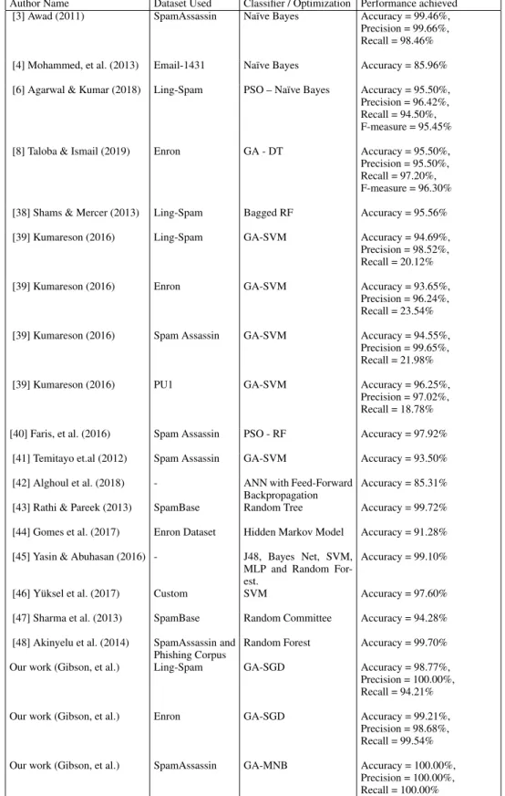
Table-21 shows the comparison of this work with similar work of other researchers. The table includes 15 additional papers similar to our paper. Some of the research work have defined additional measurements with accuracy. Majority of our work when compared to the others, provided either better accuracy or similar scores. The table displays the highest accuracies based on the datasets for our work and this is presented at the bottom of the table.

XIII. FUTURE IMPLEMENTATION AND RECOMMENDATION

We plan to further carry out the machine learning algorithms to optimize and compare with different bio-inspired algo-rithms such as Firefly, Bee Colony and Ant Colony Opti-mization as researched in the previous sections. We could also explore the Deep learning Neural Network with PSO and GA by exploring different libraries such as TensorFlow’s DNN Classifier or similar.

We found that the Neural Network algorithm could have worked better with more dimension like providing broader range of values for learning rate, activation, solver, and alpha. If this project is taken further, implementation for MLP could be done through Keras or TensorFlow with GPU application. This will allow the user to input other parameters and a range of possibilities as their key values.

The user can consider implementing the PSO objective Function with RSCV to compare the difference for accuracy improvement. The PSO and GA can provide better accuracies by incorporating NLP techniques.

(19)

TABLE 21. Comparison of our work with other works

Author Name Dataset Used Classifier / Optimization Performance achieved

[3] Awad (2011) SpamAssassin Naïve Bayes Accuracy = 99.46%,

Precision = 99.66%, Recall = 98.46% [4] Mohammed, et al. (2013) Email-1431 Naïve Bayes Accuracy = 85.96% [6] Agarwal & Kumar (2018) Ling-Spam PSO – Naïve Bayes Accuracy = 95.50%,

Precision = 96.42%, Recall = 94.50%, F-measure = 95.45%

[8] Taloba & Ismail (2019) Enron GA - DT Accuracy = 95.50%,

Precision = 95.50%, Recall = 97.20%, F-measure = 96.30% [38] Shams & Mercer (2013) Ling-Spam Bagged RF Accuracy = 95.56%

[39] Kumareson (2016) Ling-Spam GA-SVM Accuracy = 94.69%,

Precision = 98.52%, Recall = 20.12%

[39] Kumareson (2016) Enron GA-SVM Accuracy = 93.65%,

[39] Kumareson (2016) Spam Assassin GA-SVM Accuracy = 94.55%,

[39] Kumareson (2016) PU1 GA-SVM Accuracy = 96.25%,

Precision = 97.02%, Recall = 18.78% [40] Faris, et al. (2016) Spam Assassin PSO - RF Accuracy = 97.92%

[41] Temitayo et.al (2012) Spam Assassin GA-SVM Accuracy = 93.50% [42] Alghoul et al. (2018) - ANN with Feed-Forward

Backpropagation

Accuracy = 85.31% [43] Rathi & Pareek (2013) SpamBase Random Tree Accuracy = 99.72% [44] Gomes et al. (2017) Enron Dataset Hidden Markov Model Accuracy = 91.28% [45] Yasin & Abuhasan (2016) - J48, Bayes Net, SVM,

MLP and Random For-est.

Accuracy = 99.10%

[46] Yüksel et al. (2017) Custom SVM Accuracy = 97.60%

[47] Sharma et al. (2013) SpamBase Random Committee Accuracy = 94.28% [48] Akinyelu et al. (2014) SpamAssassin and

Phishing Corpus

Random Forest Accuracy = 99.70%

Our work (Gibson, et al.) Ling-Spam GA-SGD Accuracy = 98.77%,

Our work (Gibson, et al.) Enron GA-SGD Accuracy = 99.21%,

Precision = 98.68%, Recall = 99.54% Our work (Gibson, et al.) SpamAssassin GA-MNB Accuracy = 100.00%,