An economic analysis of adjusted gross Revenue-Lite insurance on farm income variability for southeast Kansas farms

(1)

AN ECONOMIC ANALYSIS OF ADJUSTED GROSS REVENUE-LITE INSURANCE ON FARM INCOME VARIABILITY FOR SOUTHEAST KANSAS FARMS

by

ANDREW THOMAS SAFFERT

B.S., University of Wisconsin River Falls, 2005

A THESIS

submitted in partial fulfillment of the requirements for the degree

MASTER OF SCIENCE

Department of Agricultural Economics College of Agriculture

KANSAS STATE UNIVERSITY Manhattan, Kansas

2007

Approved by:

Major Professor Dr. Jeffery R. Williams

(2)

Copyright

ANDREW THOMAS SAFFERT

(3)

Abstract

In today’s production agricultural sector, managing risk is essential to insuring the economic well being and sustainability of successful enterprises. Considering the

inherent risks present in today’s agricultural arena, risk management has become the central focus of discussions for policy makers and producers alike. Therefore the objective of this research paper is to examine the impact a whole-farm adjusted gross revenue insurance risk management program (AGR-Lite) has on reducing farm income variability using historical farm level data for Southeast Kansas farms.

A panel data set of actual farm level income data was compiled to evaluate the impact of AGR-Lite on farm income variability for 219 Southeast Kansas farms. Although actual income tax records were not available annual data over the period 1993 to 2005 from the Kansas Farm Management Association was used to reproduce the essential information a farm manager would need from IRS form 1040 schedule F and inventory records to purchase AGR-Lite (Langemeier, 2003). Income distributions for each farm from 1999 to 2005 were calculated for two strategies; the farm manager did not insure and the manager insured each year using AGR-Lite as a stand-alone product. The AGR-Lite insurance strategy assumed a 75% coverage level and 90% payment rate. The income distributions were compared using three premium scenarios.

In general, the results of this study reveal participation in the AGR-Lite program, in most instances, reduced standard deviation, Coefficient of Variation (CV), and

(4)

were increased with the product. The following results reflect application of Actuarially Fair Average Rate for farms with Indemnities (AFARI), which is believed to reflect actual market performance. Additionally the following reflects results using Net Farm Income (NFI). Results reveal that purchasing AGR-Lite reduced standard deviations 7.01%, 11.34%, 0.29%, and 2.53% for total, crop, livestock, and dairy farms assuming AFARI. However beef farms were the lone category to sustain a 0.81% standard deviation increase. Despite reductions in absolute variability, relative risk (CV)

increased 18.94%, 17.12%, 53.84%, and 3.19% for total, livestock, beef, and dairy. Crop farms were the only category to generate a CV reduction (9.52%). Under AFARI crop farms generated the largest minimum increase, reducing downside risk, by 69.97%. For total and dairy farm categories average minimums increased 62.93% and 0.60%. The remaining farm categories, livestock and beef, yielded 65.07% and 57.03% reductions to average minimum.

(5)

List of Figures

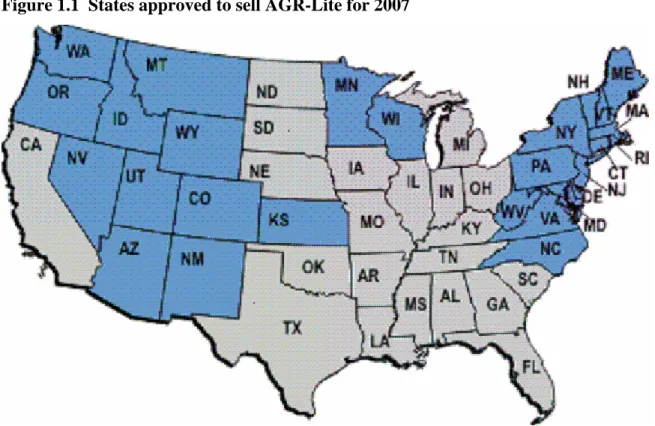
Figure 1.1 States approved to sell AGR-Lite for 2007...14

Figure 1.2 Percent of dollar coverage across federally insured designs for 2006 ...16

Figure 2.1 Acres insured under yield and revenue insurance designs from 1996 to 2006 ...42

Figure 3.1 Map of study area...45

Figure 3.2 Summary of income by category for 219 SE Kansas farms from 1993 through 2005...48

Figure 3.3 Summary of AFI, NFI, VFP, and AGRC for 219 SE Kansas Farms from 1993 through 2005 ..49

(8)

List of Tables

Table 1.1 Comparison between AGR and AGR-Lite policies...15

Table 1.2 Summary breakdown of liability by insurance design for 2006...17

Table 2.1 Summary of findings from literature review ...43

Table 3.1 Summary Statistics by farm category...50

Table 3.2 Summary of protection levels and limits and government subsidy levels...73

Table 3.3 Certainty Equivalent (CE) example calculation ...83

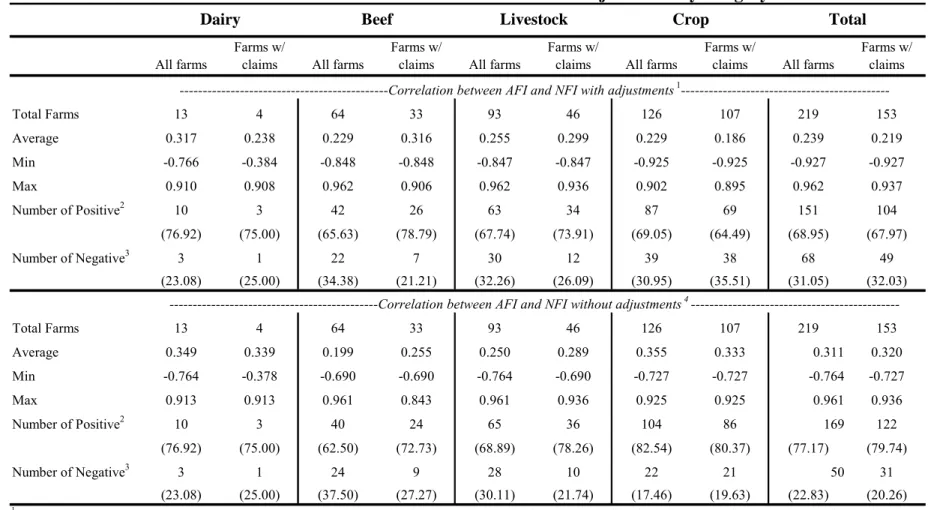
Table 3.4 Correlation coefficients between AFI and NFI with and without adjustments by category ...84

Table 3.5 Correlation coefficients between AGRC and NFI with and without adjustments by category ...85

Table 3.6 Downside risk (DR) example calculation...87

Table 4.1 Summary statistics for 219 SE Kansas farms assuming Actuarially Fair Premium by Farm (AFPF) ...144

Table 4.2 Summary by frequency of claim for 219 SE Kansas farms assuming AFPF, AFAR, and AFARI ...145

Table 4.3 Summary statistics for 153 SE Kansas farms with at least one claim assuming Actuarially Fair Premium by Farm (AFPF) ...146

Table 4.4 Summary statistics for 219 SE Kansas farms assuming Actuarially Fair Average Rate (AFAR) ...147

Table 4.5 Summary statistics for 153 SE Kansas farms with at least one claim assuming Actuarially Fair Average Rate (AFAR) ...148

Table 4.6 Summary statistics for 219 SE Kansas farms assuming Actuarially Fair Average Rate for farms with Indemnities (AFARI)...149

Table 4.7 Summary statistics for 153 SE Kansas farms with at least one claim assuming Actuarially Fair Average Rate for farms with Indemnities (AFARI) ...150

Table 4.8 Summary statistics for 126 SE Kansas crop farms assuming Actuarially Fair Premium by Farm (AFPF) ...151

Table 4.9 Summary by frequency of claim for 126 SE Kansas crop farms assuming AFPF, AFAR, and AFARI ...152

Table 4.10 Summary statistics for 107 SE Kansas crop farms with at least one claim assuming Actuarially Fair Premium by Farm (AFPF)...153

Table 4.11 Summary statistics for 126 SE Kansas crop farms assuming Actuarially Fair Average Rate (AFAR)...154

(9)

Table 4.12 Summary statistics for 107 SE Kansas crop farms with at least one claim assuming Actuarially Fair Average Rate (AFAR)...155 Table 4.13 Summary statistics for 126 SE Kansas crop farms assuming Actuarially Fair Average Rate for

farms with Indemnities (AFARI)...156 Table 4.14 Summary statistics for 107 SE Kansas crop farms with at least one claim assuming Actuarially

Fair Average Rate for farms with Indemnities (AFARI) ...157 Table 4.15 Summary statistics for 93 SE Kansas livestock farms assuming Actuarially Fair Premium by

Farm (AFPF)...158 Table 4.16 Summary by frequency of claim for 93 SE Kansas livestock farms assuming AFPF, AFAR, and AFARI ...159 Table 4.17 Summary statistics for 46 SE Kansas livestock farms with at least one claim assuming

Actuarially Fair Premium by Farm (AFPF)...160 Table 4.18 Summary statistics for 93 SE Kansas livestock farms assuming Actuarially Fair Average Rate

(AFAR)...161 Table 4.19 Summary statistics for 46 SE Kansas livestock farms with at least one claim assuming

Actuarially Fair Average Rate (AFAR) ...162 Table 4.20 Summary statistics for 93 SE Kansas livestock farms assuming Actuarially Fair Average Rate

for farms with Indemnities (AFARI) ...163 Table 4.21 Summary statistics for 46 SE Kansas livestock farms with at least one claim assuming

Actuarially Fair Average Rate for farms with Indemnities (AFARI) ...164 Table 4.22 Summary statistics for 64 SE Kansas beef farms assuming Actuarially Fair Premium by Farm

(AFPF) ...165 Table 4.23 Summary by frequency of claim for 64 SE Kansas beef farms assuming AFPF, AFAR, and

AFARI ...166 Table 4.24 Summary statistics for 33 SE Kansas beef farms with at least one claim assuming Actuarially

Fair Premium by Farm (AFPF)...167 Table 4.25 Summary statistics for 64 SE Kansas beef farms assuming Actuarially Fair Average Rate

(AFAR)...168 Table 4.26 Summary statistics for 33 SE Kansas beef farms with at least one claim assuming Actuarially

Fair Average Rate (AFAR)...169 Table 4.27 Summary statistics for 64 SE Kansas beef farms assuming Actuarially Fair Average Rate for

farms with Indemnities (AFARI)...170 Table 4.28 Summary statistics for 33 SE Kansas beef farms with at least one claim assuming Actuarially

Fair Average Rate for farms with Indemnities (AFARI) ...171 Table 4.29 Summary statistics for 13 SE Kansas dairy farms assuming Actuarially Fair Premium by Farm

(10)

Table 4.30 Summary by frequency of claim for 13 SE Kansas dairy farms assuming AFPF, AFAR, and AFARI ...173 Table 4.31 Summary statistics for 4 SE Kansas dairy farms with at least one claim assuming Actuarially

Fair Premium by Farm (AFPF)...174 Table 4.32 Summary statistics for 13 SE Kansas dairy farms assuming Actuarially Fair Average Rate

(AFAR)...175 Table 4.33 Summary statistics for 4 SE Kansas dairy farms with at least one claim assuming Actuarially

Fair Average Rate (AFAR)...176 Table 4.34 Summary statistics for 13 SE Kansas dairy farms assuming Actuarially Fair Average Rate for

farms with Indemnities (AFARI)...177 Table 4.35 Summary statistics for 4 SE Kansas dairy farms with at least one claim assuming Actuarially

Fair Average Rate for farms with Indemnities (AFARI) ...178 Table 4.36 Summary statistics for 33 SE Kansas crop farms with Value of Farm Production (VFP) of less

than $100,000 assuming Actuarially Fair Premium by Farm (AFPF) ...179 Table 4.37 Summary by frequency of claim for 33 SE Kansas crop farms with Value of Farm Production

(VFP) of less than $100,000 assuming AFPF, AFAR, and AFARI...180 Table 4.38 Summary statistics for 26 SE Kansas crop farms with Value of Farm Production (VFP) of less

than $100,000 with at least one claim assuming Actuarially Fair Premium by Farm (AFPF)...181 Table 4.39 Summary statistics for 33 SE Kansas crop farms with Value of Farm Production (VFP) of less

than $100,000 assuming Actuarially Fair Average Rate (AFAR) ...182 Table 4.40 Summary statistics for 26 SE Kansas crop farms with Value of Farm Production (VFP) of less

than $100,000 with at least one claim assuming Actuarially Fair Average Rate (AFAR)...183 Table 4.41 Summary statistics for 33 SE Kansas crop farms with Value of Farm Production (VFP) of less

than $100,000 assuming Actuarially Fair Average Rate for farms with Indemnities (AFARI)...184 Table 4.42 Summary statistics for 26 SE Kansas crop farms with Value of Farm Production (VFP) of less

than $100,000 with at least one claim assuming Actuarially Fair Average Rate for farms with

Indemnities (AFARI)...185 Table 4.43 Summary statistics for 49 SE Kansas crop farms with Value of Farm Production (VFP) of

$100,000 to $249,999 assuming Actuarially Fair Premium by Farm (AFPF) ...186 Table 4.44 Summary by frequency of claim for 49 SE Kansas crop farms with Value of Farm Production

(VFP) of $100,000 to $249,999 assuming AFPF, AFAR, and AFARI ...187 Table 4.45 Summary statistics for 44 SE Kansas crop farms with Value of Farm Production (VFP) of

$100,000 to $249,999 with at least one claim assuming Actuarially Fair Premium by Farm (AFPF) ...188 Table 4.46 Summary statistics for 49 SE Kansas crop farms with Value of Farm Production (VFP) of

(11)

Table 4.47 Summary statistics for 44 SE Kansas crop farms with Value of Farm Production (VFP) of $100,000 to $249,999 with at least one claim assuming Actuarially Fair Average Rate (AFAR) ....190 Table 4.48 Summary statistics for 49 SE Kansas crop farms with Value of Farm Production (VFP) of

$100,000 to $249,999 assuming Actuarially Fair Average Rate for farms with Indemnities (AFARI) ...191 Table 4.49 Summary statistics for 44 SE Kansas crop farms with Value of Farm Production (VFP) of

$100,000 to $249,999 with at least one claim assuming Actuarially Fair Average Rate for farms with Indemnities (AFARI)...192 Table 4.50 Summary statistics for 38 SE Kansas crop farms with Value of Farm Production (VFP) of

$250,000 to $500,000 assuming Actuarially Fair Premium by Farm (AFPF) ...193 Table 4.51 Summary by frequency of claim for 38 SE Kansas crop farms with Value of Farm Production

(VFP) of $250,000 to $500,000 assuming AFPF, AFAR, and AFARI ...194 Table 4.52 Summary statistics for 33 SE Kansas crop farms with Value of Farm Production (VFP) of

$250,000 to $500,000 with at least one claim assuming Actuarially Fair Premium by Farm (AFPF) ...195 Table 4.53 Summary statistics for 38 SE Kansas crop farms with Value of Farm Production (VFP) of

$250,000 to $500,000 assuming Actuarially Fair Average Rate (AFAR) ...196 Table 4.54 Summary statistics for 33 SE Kansas crop farms with Value of Farm Production (VFP) of

$250,000 to $500,000 with at least one claim assuming Actuarially Fair Average Rate (AFAR) ....197 Table 4.55 Summary statistics for 38 SE Kansas crop farms with Value of Farm Production (VFP) of

$250,000 to $500,000 assuming Actuarially Fair Average Rate for farms with Indemnities (AFARI) ...198 Table 4.56 Summary statistics for 33 SE Kansas crop farms with Value of Farm Production (VFP) of

$250,000 to $500,000 with at least one claim assuming Actuarially Fair Average Rate for farms with Indemnities (AFARI)...199 Table 4.57 Summary statistics for 6 SE Kansas crop farms with Value of Farm Production (VFP) of

greater than $500,000 assuming Actuarially Fair Premium by Farm (AFPF) ...200 Table 4.58 Summary by frequency of claim for 6 SE Kansas crop farms with Value of Farm Production

(VFP) of greater than $500,000 assuming AFPF, AFAR, and AFARI...201 Table 4.59 Summary statistics for 4 SE Kansas crop farms with Value of Farm Production (VFP) of

greater than $500,000 with at least one claim assuming Actuarially Fair Premium by Farm (AFPF) ...202 Table 4.60 Summary statistics for 6 SE Kansas crop farms with Value of Farm Production (VFP) of

greater than $500,000 assuming Actuarially Fair Average Rate (AFAR) ...203 Table 4.61 Summary statistics for 4 SE Kansas crop farms with Value of Farm Production (VFP) of

(12)

Table 4.62 Summary statistics for 6 SE Kansas crop farms with Value of Farm Production (VFP) of greater than $500,000 assuming Actuarially Fair Average Rate for farms with Indemnities (AFARI)

...205 Table 4.63 Summary statistics for 4 SE Kansas crop farms with value of farm production (VFP) of greater

than $500,000 with at least one claim assuming Actuarially Fair Average Rate for farms with

Indemnities (AFARI)...206 Table 4.64 Summary statistics of rates and premiums for SE Kansas farms by farm category ...207 Table 4.65 Summary statistics of rates and premiums for SE Kansas crop farms by Value of Farm

Production (VFP)...208 Table 4.66 Certainty Equivalent (CE) analysis assuming a logarithmic utility function for AFPF for all

farms and farms with at least one claim...209 Table 4.67 Certainty Equivalent (CE) analysis assuming a logarithmic utility function for Actuarially Fair

Average Rate (AFAR) for all farms and farms with at least one claim ...210 Table 4.68 Certainty Equivalent (CE) analysis assuming a logarithmic utility function for Actuarially Fair

Average Rate for farms with Indemnities (AFARI) for all farms and farms with at least one claim 211 Table 4.69 Certainty Equivalent (CE) analysis of crop farms assuming a logarithmic utility function under

Actuarially Fair Premium by Farm (AFPF) by Value of Farm Production (VFP) for all farms and farms with at least one claim ...212 Table 4.70 Certainty Equivalent (CE) analysis for crop farms assuming a logarithmic utility function under

Actuarially Fair Average Rate (AFAR) by Value of Farm Production (VFP) for all farms and farms with at least one claim ...213 Table 4.71 Certainty Equivalent (CE) analysis for crop farms assuming a logarithmic utility function under

Actuarially Fair Average Rate for Farms with Indemnities (AFARI) by Value of Farm Production (VFP) for all farms and farms with at least one claim ...214 Table 4.72 Downside Risk (DR) analysis for all farms assuming Actuarially Fair Average Rate (AFAR)

...215 Table 4.73 Downside Risk (DR) analysis for farms with at least on claim assuming Actuarially Fair

Average Rate (AFAR) ...216 Table 4.74 Downside Risk (DR) analysis for all farms assuming Actuarially Fair Average Rate for farms

with Indemnities (AFARI)...217 Table 4.75 Downside Risk (DR) analysis for farms with at least one claim assuming Actuarially Fair

Average Rate for farms with Indemnities (AFARI) ...218 Table 4.76 Downside Risk (DR) analysis for crop farms assuming Actuarially Fair Average Rate (AFAR)

by Value of Farm Production (VFP)...219 Table 4.77 Downside Risk (DR) analysis for crop farms with at least one claim assuming Actuarially Fair

(13)

Table 4.78 Downside Risk (DR) analysis for crop farms assuming Actuarially Fair Average Rate for farms with Indemnities (AFARI) by Value of Farm Production (VFP) ...221 Table 4.79 Downside Risk (DR) analysis for crop farms with at least one claim assuming Actuarially Fair

Average Rate for farms with Indemnities (AFARI) by Value of Farm Production (VFP) ...222 Table 5.1 Summary of risk measures for AFPF, AFAR, and AFARI by farm category including all farms

for Net Farm Income (NFI)...245 Table 5.2 Summary of risk measures for AFPF, AFAR, and AFARI by farm category for farms with at

least one claim for Net Farm Income (NFI)...246 Table 5.3 Summary of risk measures for AFPF, AFAR, and AFARI for crop farms by Value of Farm

Production (VFP) for all farms for NFI ...247 Table 5.4 Summary of risk measures for AFPF, AFAR, and AFARI for crop farms by Value of Farm

Production (VFP) for farms with at least one claim for Net Farm Income (NFI)...248 Table 5.5 Certainty Equivalent (CE) summary by farm category for all farms and farms with at least one

claim for AFPF, AFAR, and AFARI ...249 Table 5.6 Certainty Equivalent (CE) summary for VFP categories for all farms and farms with at least one

claim for AFPF, AFAR, and AFARI ...250 Table 5.7 Downside Risk (DR) summary by farm category for all farms and farms with at least one claim

for AFAR and AFARI*_...251

Table 5.8 Downside Risk (DR) summary of crop farms for all farms and farms with at least one claim for AFAR and AFARI for VFP categories*_...252

(14)

Acknowledgements

I would like to take this opportunity to acknowledge a number of individuals who contributed to my accomplishments and success throughout my graduate study at Kansas State University.

First I would like to extend my sincere appreciation to my major professor, Dr. Jeff Williams. His consistent support and guidance helped me to learn much along this journey in developing this thesis and pursuit of a Master’s degree. In addition I would like to extend my genuine gratitude to the other committee members Dr. G. Art Barnaby for all his expertise and knowledge of the insurance industry and Dr. Michael Langemeier for all his work creating and developing the data used in this thesis.

Outside of my committee, I would like to give recognition to Jon Newkirk, John Nelson, Rebecca Davis, and Dave Paul for their assistance in rate development for AGR-Lite in Kansas and responding to the technical questions regarding the AGR-AGR-Lite policy. A special thanks to the Kansas Farm Management Association extension Ag Economists for all their work collecting the data over the years that were used in this thesis. Finally I would like to acknowledge Frontier Farm Credit, Farm Credit Services of Central

Kansas, Farm Credit of Western Kansas, and Farm Credit of SW Kansas.

Additionally, I want to thank the staff and my fellow colleagues. I have learned much and developed great friendships with each of you. You provided assistance and guidance when needed and I am forever appreciative for that. It has been a pleasurable experience to work with each and every one of you.

(15)

Finally I would like to thank my parents for believing in me and supporting me in all my endeavors. I would not be where I am today or achieved what I have without their continued support and guidance. Lastly, I want to thank my fiancée, who has been a continual source of support, encouragement, and love throughout the pursuit of my graduate degree.

(16)

CHAPTER 1 - Introduction

1.1 Overview

In today’s production agricultural sector, managing risk is essential to insuring the economic well being and sustainability of successful enterprises. Despite the inherent and inescapable presence of risk in agriculture, some risk is manageable. Risk

management is not addressed as a single solution nor does it operate with defined set of procedures that inoculates a farm against risk. In this uncertain and unpredictable environment in which farm managers and policy makers operate, mechanisms employed to mitigate risk must continually undergo modifications as the face of agriculture

continues to change. Farm managers purchase crop and livestock insurance as a means of insulating themselves from environmental and economic shocks, predominantly related to production, price, and revenue variability. Yield variability exists due to the presence and uncertainty in weather, diseases, insects, and other pests, which

subsequently triggers volatility in market prices (Gray, Richardson, and McClaskey, 1995). In addition to environmental factors, shocks to market supply and demand, both domestically and internationally, create heightened volatility in market prices. Given the previous scenario and the inherent inelastic demand of agricultural products, risk

associated with price is further exacerbated. Historically crop and livestock insurance has provided valuable risk management by transferring production risk to insurance providers who are reinsured by the Risk Management Agency (RMA). Government programs implemented through the Farm Service Agency (FSA) provide a stabilizing mechanism and limit the degree and severity to which producers experience variability in

(17)

farm prices, yields/production, and income. Gray, Richardson, and McClaskey contend the transfer of risk to government stems primarily from, “the inherent instability of farms prices and income” which have been the leading motivators in justifying government intervention (1995).

According to the Insurance Information Institute, “crop insurance has become the largest single source of financial protection to farmers”, which in 2005 insured nearly 250 million acres (2006). As legislation begins for the 2007 Farm Bill, many economists anticipate a transition from the traditional income enhancement approach to one focusing on and promoting risk management. Government spending on U.S. farm programs has shifted from primarily price supports to one focusing on risk management. In the future we can expect to see a greater reallocation of government spending toward programs targeting risk management.

1.2 History of U.S. Crop and Livestock Insurance Program

The Federal Crop Insurance Corporation (FCIC), an organization within the United States Department of Agriculture (USDA), first debuted following ratification of the Agricultural Adjustment Act of 1938. Their objective aimed to devise and implement an organization which promoted improvement of the agriculture sector through

development of crop insurance. Furthermore the objective was to reduce individual losses associated with unavoidable perils through an actuarially sound risk management program. The Crop Insurance Act of 1980 set out to coordinate a partnership between private and public sectors. This partnership eventually led to the expansion of numerous county crop programs implemented through the private sector. It was through this partnership which allowed for the development of an efficient and effective program.

(18)

From 1981 to 1990 insured acres soared from a reported 45 million to 101 million attributed to cheaper insurance as a result of subsidies. Despite such success, disaster assistance ballooned in the 1980’s attributed to severe droughts in ’81, ’88, and ’89. Even with efforts to eliminate disaster payments congress has continually provided disaster assistance to farmers with recent notable outlays in 2003 and 2004. It was the Crop Insurance Reform Act of 1994 which mandated participation for eligibility for additional government payments (i.e. deficiency payments). Farmers were now offered the option of a catastrophic insurance coverage for a minimal administrative fee. Congress’s goal for insurance to become the primary vehicle for providing assistance to farmers, away from ad hoc disaster assistance, was slowly becoming a reality as

participation rates reached all time highs. More recently, under the provisions of the Federal Agriculture Improvement and Reform (FAIR) Act of 1996, RMA was assembled to execute and supervise programs authorized under FCIC. According to RMA, their mission is to, “Promote, support, and regulate sound risk management solutions to preserve and strengthen the economic stability of America’s agricultural producers (RMA, 2005).” As of 2003, 22 RMA reinsured crop insurance plans existed, covering over 100 commodities and insuring 218 million plus acres. According to the RMA website, in 2005, just over 16.4 million acres were insured in Kansas, accounting for nearly 71% of total acreage committed to field and miscellaneous crops.

1.3 Yield Based Contracts

Yield based contracts dominated the insurance industry until the early 1990’s. Multiple Peril Crop Insurance (MPCI) more recently referred to as APH, the longest running insurance design, provides comprehensive coverage of unavoidable perils and

(19)

other losses including but not limited to, costs associated with prevented planting, replanting, and late planting. These contracts provide protection for individual

commodities. MPCI covers nearly 70 commodities with coverage levels from 50% to 85% with payout elections of 55% to 100% of expected market price. Indemnities are issued when harvested yield falls below the yield guarantee, determined by the producers Actual Production History (APH). APH is computed as a per acre average yield using a minimum of 4 and maximum of 10 consecutive crop years of past yields for the insured commodity. When less than four years of actual, temporary, and/or assigned yields are unavailable transitional yields are used in calculating average or approved APH yields. Low yields can be replaced with 60% of the transitional yield or farmers may select “yield cups” to limit reduction in the APH as result of multiple year losses. The yield guarantee is derived from the product of APH and producer chosen coverage level.

Another yield based contract, Group Risk Plan (GRP), is a management tool which determines losses based on a county index, irrespective of individual yields. GRP was introduced with hopes of addressing the inherent problems of adverse selection and moral hazard present in current insurance programs. Features of GRP include less paperwork, lower loss adjustment expenses, and lower overall administrative costs. When actual county yield of the insured commodity, published by National Agricultural Statistics Service (NASS) and approved by RMA, falls below the trigger yield,

indemnities are issued in accordance with producer’s elected coverage level ranging from 70% to 90% in 5% increments and selected protection level. The trigger yield or

coverage level is derived by multiplying expected county yield and producer chosen coverage level. Protection level for GRP, selected by the producer, is equated by

(20)

multiplying the percent revenue coverage, 60% to 100%, and maximum dollars of protection per acre. Maximum dollars of protection is derived from the product of expected county yield, GRP price, and 150%.

1.4 Revenue Based Contracts

Up until the early 1990’s, FCIC had sufficiently covered yield risk for many crops (under MPCI policies), however products addressing or associated with price risk did not exist. Federally insured crop programs endured a series of changes including the

introduction of insurance designs protecting producers from low prices, low yields, or a combination of the two. Revenue insurance designs enabled producers to manage price and yields through the guarantee of a predetermined revenue level. Consistent with yield based designs, the following programs provide protection for individual commodities. Income Protection (IP) and Crop Revenue Coverage (CRC) were introduced in 1996 with Revenue Assurance (RA) debuting in 1997. Collectively these policies protect producers against revenue deficiencies attributed to unfavorable prices and yields. IP, developed by the USDA and based on APH, protects producers from reductions in gross revenue and distributes indemnities when gross revenue falls below the revenue guarantee. The product of APH yield, base market price, and coverage level, equates a producer’s revenue guarantee. Producers can elect coverage levels from 50% to 75% in 5%

increments. Individual gross revenue equals harvest or actual yield times harvest price. Developed by American Agrisurance, CRC protects against low yields and low prices or a combination of the two. Following CRC provisions, indemnities will be disbursed when gross revenue falls below the revenue guarantee. The final revenue guarantee is calculated by multiplying producer APH by selected coverage level by the

(21)

higher of harvest price (which reflect market conditions at harvest time) or base price (determined prior to insurance purchase). Given the previous provision, CRC provides producers with upside as well as downside price protection. Coverage levels range from 50% to 85% in 5% increments. The producer’s gross revenue to count equals the actual harvested yield multiplied by harvest price.

Iowa Farm Bureau developed RA, which similar to alternative revenue insurance designs, protects producers against unfavorable market prices and production

shortcomings. Indemnities are received when the dollar value of production falls below the revenue guarantee. Per-acre revenue guarantee is the product of APH, higher of base price or harvest price, and the selected coverage level. Producers can select from a range of coverage for approved average yield from 65% to 85% in 5% increments. Following harvest, revenue to determine any payments is simply yield per acre multiplied by fall harvest price.

In 1999, Group Risk Income Protection (GRIP), recognized as the revenue component of GRP, debuted protecting producers on the basis of expected county gross revenue per acre of the insured commodity, irrespective of individual gross revenue. Producers receive indemnities when actual county gross revenue, computed by the product of actual county yield and harvest price, falls below some predetermined trigger revenue. Individual trigger revenue is equated by multiplying expected price, expected yield, and coverage level (ranging from 70% to 90% in 5% increments) of the insured commodity.

Introduced in 1999, Adjusted Gross Revenue (AGR) became the first revenue product insuring a percentage of average gross revenue for the entire farm. Currently

(22)

AGR is available in 18 states across the U.S however USDA has frozen further expansion of AGR. AGR provides coverage under one policy for multiple agricultural

commodities. Motivation for AGR was to provide insurance based on current and historical tax records, specifically Schedule F 1040 filings or equivalent tax forms. With the use of federal tax records, RMA believes this approach will “reinforce program credibility by using IRS forms and regulations to ensure compliance (RMA, 2003).”

1.5 Livestock Insurance

The Agricultural Risk Protection Act (ARPA) of 2000 gave the green light to develop federally reinsured livestock products. Prior to the enactment of ARPA, livestock remained a sector effectively excluded from RMA risk management programs specifically insurance. November 15, 2001 marked FCIC approval of federally reinsured livestock products known as Livestock Risk Protection (LRP) for swine, fed cattle, and feeder cattle. The basis of LRP is to protect producers against falling market prices, below some predetermined coverage price. Key features of LRP include coverage levels ranging from 70% to 95% of expected ending value and the flexibility to purchase insurance coinciding with individual marketing periods and number of actual insured livestock. Indemnities are paid when actual ending value, a weighted average price of the insured livestock, reported by Chicago Mercantile Exchange (CME), falls below the chosen coverage price. Taking expected ending value, reported daily on the RMA

website, and multiplying by producer chosen coverage percentage, establishes a coverage price protecting producers on a dollar per cwt basis.

Livestock Gross Margin (LGM) protects against producer shortcomings in gross margin which is simply livestock market value minus feed costs. Available coverage

(23)

levels range from 80% to 100% in 5% increments. Producers receive indemnities equal to the difference, between actual gross margin and guaranteed gross margin if positive. Actual gross margin is the product of total target marketings and actual gross margin of the insured livestock. Gross margin guarantee is derived by the product of expected total gross margin and chosen coverage level. Multiplying target marketings, as determined by the producer, by expected gross margin per livestock unit for each month and summing the values, equates expected total gross margin. Expected gross margin per livestock unit is established by subtracting expected feed cost, specified under LGM provisions, from the product of expected marketing month price, reported by CME, and marketing weight of the insured livestock.

1.6 Whole-Farm Revenue Insurance

In 2003, Adjusted Gross Revenue-Lite (AGR-Lite) was introduced. Designed with the parent program (AGR) in mind, this insurance program has a more simplified design continuing revenue protection for the whole-farm for all crop and livestock enterprises. AGR-Lite was first developed by the Pennsylvania Department of

Agriculture and for 2007 is available for sale in 28 states (AK, AZ, CO, CT, DE, ID, KS, MA, MD, ME, MN, MT, NC, NH, NJ, NM, NV, NY, OR, PA, RI, UT, VA, VT, WA, WI, WV, and WY). Figure 1.1 illustrates those states which are approved to sell AGR-Lite.

To encourage participation, maximum total liability approved for AGR-Lite for insurance year 2006 was increased from $250,000 to $1,000,000. However, liability is still substantially less than the maximum liability currently offered by AGR ($6,500,000). One other distinctive feature of AGR-Lite was the elimination of the livestock restriction.

(24)

AGR limits the maximum share of livestock and livestock product revenue in the

guarantee to 35% and AGR-Lite does not. Table 1.1 provides a comparison of the AGR and AGR-Lite programs. For further information on AGR and AGR-Lite refer to the following RMA websites:

¾ http://www.rma.usda.gov/pubs/2003/PAN-1667-06rev2.pdf ¾ http://www.rma.usda.gov/pubs/2003/PAN-1667-07.pdf

When comparing alternative insurance designs, AGR-Lite may be used as a standalone product or as an umbrella (wrap around) policy allowing producers to use AGR-Lite in conjunction with alternative crop insurance designs, excluding AGR. Farmer paid premiums for AGR-Lite will be reduced when producers purchase additional insurance products, which reduce total liability. However, a producer may not

accumulate indemnities from all insured products in excess of the total value of their losses.

Limitations of AGR-Lite specify that a qualifying person can generate no more than 50% of their total revenue from commodities purchased for resale. An example would be the purchase of grapes to be converted into wine. Potato revenue must not exceed 83.35% of their revenue stream. It is important to note the resale limitation does not apply to commodities purchased for further growth, such as stockers, cattle

backgrounded, and fed cattle.

Producers are able to select from three coverage levels (65%, 75%, and 80%) of average gross revenue with an indemnity payment rate of 75% and 90%. For 2006 virtually all producers will qualify for 65% and 75% coverage levels with a one commodity requirement. To qualify for higher coverage levels (80%), producers must

(25)

indicate on their intended agricultural commodity report that at least three agricultural commodities will be produced whose expected income will be greater than or equal to that determined by the diversification formula. The intended agricultural commodity report will be submitted at the beginning of each eligible insurance year and details the commodity, expected acreage, yield, expected value, and total value. The policy also requires that qualifying persons submit a minimum of five years of continuous, verifiable tax records for the same entity, preferably Schedule F 1040 filings or equivalent tax forms to document historical revenue and expenses.

To encourage participation in AGR-Lite RMA pays 59%, 55%, and 48% of the total premium for coverage levels of 65%, 75%, and 80% respectively. Calculations for revenue guarantee are derived from the lesser of the 5-year average gross revenue based on tax returns or the expected farm income times the producer’s elected coverage level percentage. When a producer realizes a shortfall in gross revenue, below the guarantee level, an indemnity is paid based on the producers selected payment rate percentage.

AGR-Lite provides protection for otherwise uninsurable commodities such as organic and direct marketed production; provides farm operations with a bottom line from severe economic loss; provides individual protection based on personal yield, price history, plus low price protection; and finally it may provide an alternative for farms with reduced APH caused by multiple years of crop losses.

AGR-Lite possesses great potential in filling the voids or gaps in the current FCIC product line as this product caters to small, diversified, livestock, and specialty crop firms. Despite such potential, the market for AGR-Lite in approved states has struggled as the following will illustrate. In 2003 74 policies were sold with subsequent year sales

(26)

of 88 in 2004, 162 in 2005, and an unofficial 348 in 2006. Refer to Figure 1.2 for a breakdown of crop insurance activity for 2005 production year. Furthermore Table 1.2 provides a numerical summary of liability by insurance design. Reasons or speculations for such stagnant sales include the initial maximum liability of $250,000 which has since been raised to $1,000,000. Furthermore, in a statement by Keith Collins, Chief

Economist at the USDA argues that poor participation levels may be attributed to, “the learning curve of a financial product as compared to a production agricultural type of insurance product, as well as the cost of delivery (2005).” Since its debut in 2003, AGR-Lite has undergone several revisions and in light of recent complaints, will continue to do so.

1.7 Research Objective

According to NASS census data for 2002, Kansas’s top six commodities (by production value) account for $8.65 billion or 98.8 percent of the state’s agricultural production. However, only one of these commodities is currently insurable: Grains, $2.1 billion attributing to 24 percent of Kansas’s agricultural production. The uninsurable commodities in the top six (by production value) are cattle and calves, $5.7 billion; hogs, $297.5 million; milk and other dairy, $248.5 million; hay and other production, $225 million; and nursery and greenhouse, $55.5 million. These uninsurable commodities account for $6.55 billion or over 74 percent of agricultural production currently without risk protection. These statistics further substantiate the need for analysis of AGR-Lite in Kansas agriculture.

Given the previous statistics, the objective of this research is to establish the impact of participation in AGR-Lite for SE Kansas farms on income variability.

(27)

Potential risk reduction associated with AGR-Lite will also be estimated. Five categories of farms are used to examine the impact of AGR-Lite on adjusted gross revenue to count (AGRC) and net farm income (NFI) variability. Categories used for analysis include all farms, crop farms, livestock farms, beef farms, and dairy farms. The farms were placed into each category if they averaged 50% or more of total income from crop, livestock, beef, or dairy over the 13 years. The Kansas Farm Management Association (KFMA) data was used to compile 13 years (1993-2005) of continuous farm level data that was used to evaluate participation in AGR-Lite. The primary objective of this study evaluates individual farm performance assuming farms participated in AGR-Lite. A more detailed and specific list of objectives for this study follow:

1. Establish an area of study, study period, and compile a panel data set of farm level data

2. Determine farm type categories for analysis.

3. Summarize the trend in the data for selected income variables. 4. Formulate a mathematical representation of the AGR-Lite policy.

5. Define procedures to estimate actuarially fair premiums that correspond to the policy.

6. Identify risk analysis procedures and statistics for comparison including standard deviation, Coefficient of Variation (CV), minimums, maximums, Downside Risk (DR), and Certainty Equivalents (CE).

7. Identify data limitations that caused revision of the procedures to calculate the income distributions with and without participation in AGR-Lite. 8. Estimate gross and net income distributions with and with out the

AGR-Lite policy under three premium calculation procedures. 9. Compare the previously identified statistics from the estimated

distributions to determine the overall impact of AGR-Lite by farm

category as well as Value of Farm Production (VFP) levels for crop farms, over all farms and farms with claims.

(28)

1.8 Chapter Outline

An outline describing the remaining contents of the thesis will follow. Chapter 2 reviews prior literature which has analyzed many of the current Federal Crop Insurance Corporation programs and their effectiveness at mitigating risk. Chapter 3 describes the data, methods, and assumptions used to conduct the analysis. Chapter 4 presents the results of the analysis. A brief summary of findings, research limitations, discussion of future research and concluding comments are presented in Chapter 5.

(29)

Figure 1.1 States approved to sell AGR-Lite for 2007

(30)

Table 1.1 Comparison between AGR and AGR-Lite policies

AGR* AGR-Lite

Maximum Liability $6,500,000 $1,000,000

Animal and Animal Product Limit 35% N/A

Purchased For Resale1 <50% <50%

Coverage Level (%)2 _{65, 75, 80} _{65, 75, 80}

Payment Rate (%) 75, 90 75, 90

Government Subsidy (%)3 48, 55, 59 48, 55, 59

Note: Adjusted Gross Revenue (AGR), Adjusted Gross Revenue-Lite (AGR-Lite)

3_{Government subsidy levels are 48%, 55%, and 59% for coverage levels of 80%, 75%, and 65% respectively} *_{AGR is currently unavailable in Kansas and will not be available in the succeeding crop year}

1_{Producer must not generate more than 50% of gross income from resale commodities. This does not include}

commodities purchased for further growth.

2_{There are minimum commodity requirements for each of the coverage level percentages. Each commodity must}

(31)

16

Figure 1.2 Percent of dollar coverage across federally insured designs for 2006

GRIP - Group Risk Income Protection

11% GRP - Group Risk Plan

2% Livestock Gross Margin

(LGM) & Livestock Risk Protection (LRP) 0% Revenue Insurance1 47% Other Products2 13%

APH - Actual Production History

26% AGR - Adjusted Gross

Revenue

1% AGR-Lite - Adjusted Gross

Revenue-Lite 0%

(32)

Table 1.2 Summary breakdown of liability by insurance design for 2006

Insurance Plan Liability

AGR - Adjusted Gross Revenue $293,767,147

AGR-Lite - Adjusted Gross Revenue-Lite $57,072,794

APH - Actual Production History $12,950,628,237

GRIP - Group Risk Income Protection $5,733,025,928

GRP - Group Risk Plan $1,051,980,975

Livestock Gross Margin (LGM) & Livestock Risk Protection (LRP) $189,561,978

Revenue Insurance1 $23,466,898,287

Other Products2 $6,331,318,483

Total $50,074,253,829

1_{Other Products Include: Aquaculture Dollar (AQU), Avacodo Revenue Coverage (ARC), Dollar Plan (DOL), Indexed APH}

(IAPH), Income Protection (IP), Indexed IP (IIP), Pecan Revenue (PRV), Tree Based Dollar Amount (TDO), Yield Based Dollar Amount (YDO)

2_{Revenue insurance combines liability from Revenue Assurance (RA) and Crop Revenue Coverage (CRC).}

Source: USDA, RMA at http://www3.rma.usda.gov/apps/sob/current_week/insplan2006.pdf and

(33)

CHAPTER 2 - Literature Review

2.1 Introduction

Exploring the use of crop insurance as a risk management instrument and its significance in the agricultural industry has been widely researched. With concerns from taxpayers regarding the costs of such safety net programs and increasing levels of

subsidization, there has been a renewed interest in evaluating performance of insurance designs and their effectiveness as risk reducing mechanisms. Section 2.2 and 2.3 review literature focused on performance of revenue based, as well as individual and area yield designs using farm level performance measures. Section 2.4 reviews literature

conducting cross comparison analysis between yield and revenue based schemes. Each section will provide detail on the methods employed in capturing the effectiveness and efficiency of federally endorsed insurance mechanisms and discuss significant findings of each.

2.2 Revenue Based Designs

Prior to presenting literature which analyzed revenue based designs, the following section discusses an article from Dismukes and Coble (2006) which contends revenue insurance may be more effective in risk management compared to alternative methods. Since introducing revenue based designs in 1996, participation has surpassed yield based designs covering over 57% of insured acreage. Figure 2.1 illustrates the transition from traditional yield based coverage to revenue based from 1996 to 2006. One key driver contributing to increased participation has been government subsidized

(34)

premiums. According to Dismukes and Coble (2006) government paid subsidies for revenue insurance in 2006 totaled $1.8 billion, exceeding producer paid premium by $400 million. Revenue insurance provides coverage for intra-season not inter-season, thus guarantee levels will more accurately reflect market conditions, ultimately limiting the presence of market distortion.

Unlike yield based designs, revenue oriented programs, according to Dismukes and Coble (2006), can be more effective as an income stabilizer due to the inherent characteristics of the design. First, it provides protection from loss in revenue rather than price or yield. Secondly revenue based designs are larger in scope in that dissimilar from individual designs, which only provide protection for individual segments of agriculture, revenue insurance establishes a common denominator regardless of farm composition.

Despite attractive features detailed above, Dismukes and Coble (2006) contend revenue insurance likely fails to offer “adequate coverage” as perceived by policy developers and farmers. First, unlike yield insurance, revenue products combine risks associated with yield and price, and given the highly negative correlation observed with price and yield; revenue insurance offsets the risks resulting in less variability leading to less frequent and often smaller indemnities. As such, producers often prefer purchasing separate insurance protection. Secondly, insurance often requires the insured to absorb a portion of the loss which, again, leads to the notion of “inadequate coverage” because the full value exceeds the coverage level. Lastly, is a problem that has confounded many, multiple year declines in income, to which individual and whole-farm products alike have failed to address. Multiple year declines have become the central source of contention for farmers and policy makers alike.

(35)

Gray, Richardson, and McClaskey (1995) investigated and compared the 1990 Farm Program, supporting agricultural prices through deficiency payments, acreage reduction, set-asides, and CCC loans, to two alternative schemes separate from the 1990 Farm program which proposed the following; 1) eliminate deficiency payment programs, federal crop insurance, and disaster assistance programs, 2) retain CCC non-recourse loans and Farmer-Owned reserve, and 3) eliminate all forms of acreage reduction or set-asides. These alternative schemes, developed by an Iowa Farm Bill Study Team, were called Revenue Assurance (RA) and protected producers through a guarantee of normal gross revenue at 70% and 90% coverage levels. These three alternative designs were then evaluated and compared for their effectiveness in stabilizing producer revenues and total government expenditure.

Producer gross return and government expenditure distributions were estimated through simulation models for each of the designs using eight representative farms across the nation. Estimated probability distributions enabled the authors to quantify producer support, stabilization, and government expenditures across programs. Producer gross revenue distributions were determined through Monte Carlo simulation. Ten years of national yield data were extracted to derive random national yields. In this study RA assumed protection for the whole farm, thus the process accounted for cross crop correlations within farms. Furthermore, simulations to derive correlations between national and producer yields where conducted via multivariate normal random generation (Gray, Richardson, and McClaskey, 1995). These results were then entered into a pricing formula which established a national average price. Taking national average price, multiplying by national yields, equated marketplace gross revenue. To quantify total

(36)

benefits from each design, gross revenue guarantee was computed, multiplying the five year moving average of price and yield for each crop, summing the observations, and multiplying by producer chosen coverage level (70% or 90%). Probability distributions were derived through 100 iterations for producer gross revenue and government

expenditures.

Their findings suggested that across alternative designs, the 1990 farm program supported mean producer revenues higher in comparison to RA designs. Support for mean producer revenue, assuming 90% coverage were comparable to the level supported by the 1990 farm program. Further, Gary, Richardson, and McClaskey contend the 1990 farm program to be more effective in income stabilization when price variability

constituted the principal risk confronted by the producer. On the contrary, RA provided greater income stabilization when primary revenue risk faced by producer was yield variability. When analyzing administrative costs, the 1990 farm program constituted the largest administrative outlay with 90% and 70% RA following respectively. Nationally, Gray, Richardson, and McClaskey argue, producers located in the Great Plains region (growing wheat and rice) suffer considerably under RA due to limited exposure to yield variability, resulting from irrigation and ample rainfall, and on average receive most if not all income support through components of the 1990 farm program. As for regions in the southeast and corn belt, comprised of mainly feed grain producers specifically soybeans and non-irrigated cotton, will benefit under the RA scheme, as producers receive little benefit from the 1990 farm program specifically soybean producers who received no income support under the 1990 farm program.

(37)

Hennessy, Babcock, and Hayes (1997), following the debut of revenue insurance, explored the effects of alternative revenue insurance designs to the 1990 commodity program, and no program alternatives. Specifically they investigated the effects of acreage allocations, administrative or government costs, and producer welfare across alternative policies using a representative corn and soybean farm from Sioux County Iowa.

Revenue insurance programs are broken down into individual and portfolio; then further characterized by farm or county level. These designs were then evaluated against one another for their resulting effects. The following comparisons were analyzed; revenue insurance to price and crop insurance; crop specific to portfolio designs employing state contingent approach; 1990 farm program to a no program alternative; crop specific to portfolio revenue insurance designs; and farm level revenue insurance to the 1990 farm program. Monte Carlo simulation with 5,000 iterations was used assuming prices follow a log-normal distribution and yields follow a beta distribution. The final analysis compared alternative revenue insurance designs for individual versus portfolio. Additionally producer risk preferences were assumed to be constant absolute risk

aversion.

Results suggested two important findings, first, offering revenue insurance with 75% coverage reduced government expenditures to a fraction of that under the 1990 farm program; and secondly, results were conclusive that revenue insurance offered greater protection and increased benefit irrespective of upfront expenditures. Additional findings suggested revenue insurance generated greater returns to society in comparison to the 1990 farm program. Furthermore, certainty equivalent returns (CERs), which measured

(38)

the certain return (assuming zero-risk) a producer would trade for a larger return associated with some risk. Under farm and county level revenue insurance designs, assuming 100% coverage, CERs exceeded those relative to the 1990 farm program suggesting increased producer welfare or expected income. Government expenditures were the highest under farm level crop specific revenue insurance with 100% coverage; however alternative revenue insurance designs and coverage cost less than that under the 1990 farm program.

In 2000 Miller, Coble, and Barnett investigated and compared the effectiveness of a multi-crop insurance design to individual yield and revenue insurance designs for a representative Mississippi farm. They attempted to formulate a model guaranteeing aggregate gross revenue from multiple enterprises. Cotton, soybeans, and wheat were the commodities selected for analysis. Ten combinations in total were analyzed, three

assumed 100% acreage devoted to each crop, with the remaining seven being divided across the three commodities (i.e. 50-50-0, 33-33-33, ect.).

Probability distributions were formulated, through re-sampling, via

non-parametric bootstrap simulation. County yield and historical prices from 1956-1998 were obtained from NASS. Before modeling the effectiveness of multi-crop revenue designs, equations were formulated to capture the yield variability across enterprises, and are as follows: (2.1) f ti C j C tj ij C i C ti ii f i f ti y B R R B R R e y = + ( − )+ ( − )+ where f ti

y is the yield for crop i in year t for farm f, f i

y is the mean yield for crop i on farm f, Bii and Bij are the interaction coefficients for crop i and county trend-adjusted

crop i and j, C ti

R and C i

(39)

C tj

R and C

j

R are predicted county and mean county yields for crop j, and f ti

e are the residuals for the respective crop (Miller, Coble, and Barnett, 2000). To complete the yield simulation, farm yield deviations were equated, and following simplification, are equated as: (2.2) f t f C s f s R d e y = + + where f s

y is the simulated yield for farm f, C s

R is the simulated county yield, _d f_{is the}

mean difference of yield of farm f from county yield, and f t

e is the residual for farm f in year t. Price yield relationships were equated to complete the final component required to conduct the multi-revenue simulation. Price relationships were also calculated for each crop. The subsequent equation is associated with crop i:

(2.3) 1) ( 1) ) ˆ ( 1 ( 0 1 p it C it C it p ij C it C it p ii is is R R a R R a P P = + − + − +ε where 1 is

P is the simulated price of crop i at harvest, 0

is

P is the simulated futures price at planting, p

ii

a and p

ij

a are the coefficients for deviation of county yield i from expected county yield for i and j, _C

it C it

R R

ˆ is the county yield for commodity i divided by the predicted county yield for commodity i in year t, and p

it

ε is the residual. Using equations (2.1) and (2.3), the following revenue simulation is derived:

(2.4) =

∑

i f is is i f s AP y MREV 1 where f s

MREV is the sum of revenues from multiple crops for farm f, Ai is acres planted

(40)

Using a non-parametric approach, risk reduction gains were analyzed and compared for Mississippi producers under yield, single crop revenue, and multi-crop revenue insurance designs. Certainty Equivalents (CE) were calculated, which again indicate the amount a producer would accept in lieu of some uncertain amount, and used to compare alternative insurance schemes. CE were calculated as followed:

(2.5) (1 ) ( )1 , 1 1 ≠ − = _r _E _U − _r CE r sr sr

where CEsr is the simulated CE with a risk aversion coefficient r, and E(Usr) is a

constant relative risk aversion utility function and was calculated as follows:

(2.6) , 1 1 ) ( 1 1 ≠ − =

∑

= − r r W U E s s r s s r ω

where ωs is the initial wealth and W is the ending wealth.

Under each scenario, CE increased compared to the baseline scenario of

production assuming no insurance. In some instances individual designs reported greater CE values than multi-crop designs, however Miller, Coble, and Barnett argue individual designs triggered indemnities with greater frequency compared to multi-crop schemes. All three insurance designs effectively eliminated the lower tails of revenue distributions; however, of alternative insurance schemes, multi-crop designs generated the smallest probability of low revenues.

In 2004 Gray et al. analyzed the 2001 farm program and crop revenue coverage (CRC) for what, if any impacts individual and combined mechanisms impose on the distribution of returns to land. Specifically two scenarios were analyzed, first, market returns combined with three other programs, Agricultural Market Transaction Act (AMTA) payments, Marketing Loan Payments (MLP), and Marketing Loss Assistance

(41)

(MLA) payments and secondly market returns augmented by AMTA, MLP, MLA, and CRC (Gray et al. 2004). Returns were evaluated for an Indiana crop farm operating a 50/50 rotation of corn and soybeans.

Conducting a stochastic simulation, multivariate distributions were derived for corn and soybean prices simulated in a multivariate lognormal distribution, corn and soybean yields simulated in a multivariate empirical distribution, and cumulative farm income simulated from a multivariate normal distribution. Using a budgeting model, distributions were derived under each scenario then compared against one another for their relative impact on returns to farm land. Additional criteria used in measuring impacts of alternative government payment mechanisms on the distribution of returns to land were certainty equivalents (CE). CE were calculated as follows:

(2.7) _CE ₌_[(₁₋ρ₎_EU₍_X ₊ω_)]1/(1−ρ)₋ω

where ρ is the coefficient of relative risk aversion, EU is the expected utility associated with a given return, X , and ω is the initial wealth (Gray et al. 2004). Assuming the power utility function form U follows:

(2.8) ρ ω ω ρ − + = + − 1 ) ~ ( ) ~ ( 1 X X U

and X~ was derived

(2.9) _X~ ₌_[(₁₋ρ₎_EU₍_X ₊ω_)]1/(1−ρ) ₋ω

Cash prices were procured from Indiana Agricultural Statistics Service with futures prices compiled from Chicago Board of Trade.

In comparing the two scenarios, average return to land per acre without CRC was $80.50 and $79.39 after CRC was included in the risk reducing portfolio. To reconcile

(42)

the $1.11 difference (which reflected the cost of insuring) in average returns to land, including CRC increased the bottom dollar return from $39.49 (without CRC) to $68.65, a near $30 difference; and reduced the standard deviation from $46.61 to $41.73.

Furthermore, an increase from 0.99 to 1.40 (with CRC) in skewness established the effectiveness of CRC in mitigating downward risk. For the simulated results, CE values suggested producers with greater risk aversion gained considerably compared to those associated with less risk aversion. For example, under scenario one, with no insurance assuming MLA payments, a producer with relative risk aversion of 0 observed a CE value of $16.92/acre, whereas producers with relative risk aversion 5 reported a CE value of $34.89/acre. Thus, risk reduction under MLA was more beneficial to producers with greater risk aversion. In the aggregate, producers receive greater benefits with increased risk aversion. Gray et al. contend that MLA, MLP, and AMTA, adequately removed the risk present in farming. With the addition of CRC, values were slightly higher,

insinuating greater risk reduction; however the increase is minimal suggesting that previous programs removed a significant portion of farm related risk. More importantly, this research claimed that net benefits from CRC are lessened with participation in additional government programs.

2.3 Yield Based Designs

Patrick and Rao (1989) examined the impact MPCI imposed on performance of hog –crop farms in Central Indiana. Farms were categorized by debt to asset (D/A) ratios, low, medium, and high with corresponding levels of 20%, 40%, and 70% respectively. To reflect greater yield variability experienced by farmers relative to county yields, CV were increased by 25%, 50%, and 100% of mean yields. Additional

(43)

scenarios analyzed whether or not a producer purchased MPCI, and the impacts on after-tax net present value of family withdrawals and change in net worth (ANPV), present value of ending net worth of solvent iterations (PVNW), probability of net worth gain (probability PVNW is greater than initial wealth) ( %NWG), and probability of survival (firm remains solvent for 10 year period) (%SUR). Three scenarios (MPCI assuming 1986 feedgrain and wheat program; a combination of MPCI, 1986 feedgrain and wheat program, and off farm income; or no coverage from either program) were selected and explored for the effects of increased yield variability on selected performance measures of farrow to finish hog-crop farms. Farms were further classified as having average gross farm income from $100,000 to $249,999, operated 360 acres, of which 160 is owned and 200 crop shared, and selected from corn, wheat, soybeans, or a combination of any sort.

Similar to Schumann et al. (2001), FLIPSIM was employed to investigate the impacts of various insurance designs. According to Patrick and Rao (1989), FLIPSIM is a recursive simulation model which incorporated an assortment of variables, including crop mix decisions, financial management, and marketing. Crop yield and prices were generated from multivariate normal distributions.

The first scenario analyzed the impacts of MPCI assuming 1986 feedgrain and wheat program. This scenario suggested that purchasing MPCI would in fact reduce the mean value of ANPV and PVNW under all D/A groups. Thus, participating in MPCI reduced ANPV which corresponded to a reduction in net farm income. Farm

survivability remained 100% for medium and low D/A groups. For MPCI and no 1986 feedgrain and wheat program, performance measure values were collectively worse than when augmented by the 1986 feedgrain and wheat program. Here again farms in the low

(44)

to mid D/A groups had 100% survivability. Under almost every scenario ANPV and PVNW were reduced when farmer purchased MPCI. The last scenario which included MPCI, 1986 feedgrain and wheat program, and off-farm income, suggested that an additional $12,000 of off-farm income increased ANPV, PVNW, %NWG, and %SUR under 40 and 70 percent D/A positions. Similar to previous results, ANPV and PVNW were reduced under 40% and 70% D/A with off-farm income and CV increases. Patrick and Rao concluded that for a diversified farm, as used in the study, MPCI played a trivial role in risk management due to areas of low yield variability, as is the case for Indiana hog-crop farm. In addition, participation in MPCI reduced net farm income and PVNW under a high D/A group; however engaging in MPCI yielded a positive response, albeit net farm income still declined, yet at a much smaller percentage. It is under the medium D/A group which MPCI participation has the potential to be effective. These groups benefited from increased liquidity, increased %NWG, and higher mean ANPV and PVNW values, especially under increased CV. Patrick and Rao contend that MPCI is an effective risk management tool for producers with medium D/A levels or high D/A levels with off farm income, primarily those with greater yield variability.

Miranda (1991) reevaluated area yield crop insurance, first promoted by Halcrow in 1949, questioning the effectiveness of the design in reducing yield risk with individual yield design comparisons. Furthermore, an investigation was conducted which analyzed variation across producers and techniques to optimize coverage under area yield designs. Recall that under the area yield scheme, producers will receive indemnities when area yield falls below some predetermined critical yield. Miranda discussed the theoretical aspect of area yield insurance, then, applied this framework through farm level data from

(45)

102 western Kentucky soybean farms. Although he provides no economic analysis, his discussion specifically addresses the effectiveness of these designs in yield risk reduction. He also contributed a theoretical approach which was used in other crop insurance

analysis.

To test the effectiveness of an area yield design, Miranda developed a model to measure the correlation between an individual farmer’s yield and area yields:

(10) γ~_i =μ_i+β_i(γ~−μ)+ε~_i

where γ~ is the individual farm yield, i μi is historical average farm yield,

2 ~ / ) ~ , ~ (γ γ σ_γ

βi =Cov i ; γ~ is the area yield; μ is the average area yield; and ε~ is the i

nonsystematic component. βi, which has a central tendency to one, established whether

or not area yield designs were risk reducing. The greater the β_i the higher the probability area yield designs were risk reducing. Furthermore if β_i is greater than some

criticalβ,βc, area yield is deemed risk reducing. βc were calculated as follows:

(11) ) ~ , ~ ( * 2 ~ 2 n Cov n C _γ σ β =−

where σ2n~_{is the variance of the indemnity under area yield insurance (Miranda, 1991).}

Individual yield risk, according to Miranda, can be decomposed into systematic and unsystematic components. Factors which affected producers in a selected area are captured within the systematic component while nonsystematic components are the residuals. Individual yield insurance is plagued by inherent problems of moral hazard and adverse selection. Thus, Miranda asserted, individual yield insurance is less effective due to such steep deductibles. Area yield insurance, on the other hand, is more effective as problems of moral hazard and adverse selection are limited. Results suggested that on