A Comparative Study of Bagging and Boosting of Supervised and Unsupervised Classifiers for Outliers Detection

(1)

Wright State University Wright State University

CORE Scholar

Browse all Theses and Dissertations Theses and Dissertations 2017

A Comparative Study of Bagging and Boosting of Supervised and

Unsupervised Classifiers for Outliers Detection

Yue Dang

Wright State University

Follow this and additional works at: https://corescholar.libraries.wright.edu/etd_all Part of the Electrical and Computer Engineering Commons

Repository Citation Repository Citation

Dang, Yue, "A Comparative Study of Bagging and Boosting of Supervised and Unsupervised Classifiers for Outliers Detection" (2017). Browse all Theses and Dissertations. 1814.

https://corescholar.libraries.wright.edu/etd_all/1814

This Thesis is brought to you for free and open access by the Theses and Dissertations at CORE Scholar. It has been accepted for inclusion in Browse all Theses and Dissertations by an authorized administrator of CORE

(2)

A COMPARATIVE STUDY OF BAGGING AND

BOOSTING OF SUPERVISED AND

UNSUPERVISED CLASSIFIERS FOR

OUTLIERS DETECTION

A thesis submitted in partial fulfillment

of the requirements for the degree of

Master of Science in Electrical Engineering

by

YUE DANG

B.E, University of Electronic Science and Technology of China, 2011

2017

(3)

Wright State University Graduate School

July 10 , 2017

I HEREBY RECOMMEND THAT THE THESIS PREPARED UNDER MY SUPER-VISION BY Yue Dang ENTITLED A Comparative Study of Bagging and Boosting of Supervised and Unsupervised Classifiers For Outliers Detection BE ACCEPTED IN PAR-TIAL FULFILLMENT OF THE REQUIREMENTS FOR THE DEGREE OF Master of Science in Electrical Engineering.

Zhiqiang Wu, Ph.D. thesis Director Brian Rigling, Ph.D. Department Chair Committee on Final Examination Zhiqiang Wu, Ph.D. Yan Zhuang, Ph.D. Bin Wang, Ph.D. Robert E. W. Fyffe, Ph.D. Vice President for Research and Dean of the Graduate School

(4)

ABSTRACT

Dang, Yue. M.S.E.E., Department of Electrical Engineering, Wright State University, 2017. A Comparative Study of Bagging and Boosting of Supervised and Unsupervised Classifiers For Out-liers Detection.

The problem of outlier detection has received increasing attention recently because it plays a great role in many fields such as credit fraud detection, cyber security, etc. Ma-chine Learning approach is an excellent choice for outlier detection due to its accuracy and efficiency. Outlier detection problem is unique due to the so-called classes imbalance: the inliers are extreme majority and the outliers are minority. Ensemble methods are popular in classification and regression task in practice to improve the performance of machine learn-ing algorithms. Bagglearn-ing and boostlearn-ing are two common methods of them. In this thesis, we want to show the performance of bagging and boosting compared with base algorithms in outlier detection. First of all, some basic algorithms for outlier detection are described for both supervised and unsupervised methods. Next, theoretical analysis and strategies of ensemble are discussed. Furthermore, groups of experiments are conducted and the experiment results confirm the effectiveness of bagging and boosting methods for outlier detection problem.

(5)

List of Figures

3.1 The frame of bagging . . . 16

3.2 The frame of boosting. . . 17

3.3 bias-variance dilemma . . . 20

4.1 Precision-Recall Curve . . . 24

4.2 ROC Curve . . . 25

4.3 supervised results of cardio dataset . . . 28

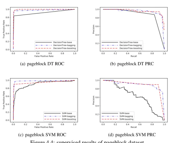
4.4 supervised results of pageblock dataset . . . 29

4.5 supervised results of wilt dataset . . . 29

4.6 supervised results of thyroid dataset . . . 30

4.7 unsupervised results of cardio dataset . . . 32

4.7 unsupervised results of cardio dataset continued . . . 33

4.8 unsupervised results of pageblock dataset . . . 34

4.8 unsupervised results of pageblock dataset continued . . . 35

4.9 unsupervised results of wilt dataset . . . 36

4.9 unsupervised results of wilt dataset continued . . . 37

4.10 unsupervised results of thyroid dataset . . . 38

(8)

List of Tables

4.1 confusion matrix . . . 23

4.2 summary of data sets . . . 26

4.3 software and hardware environment of experiments . . . 27

4.4 supervised ensemble results. . . 30

4.5 unsupervised ensemble results based on knn . . . 40

4.6 unsupervised ensemble results based on knnw . . . 40

4.7 unsupervised ensemble results based on odin . . . 40

4.8 unsupervised ensemble results based on lof . . . 41

4.9 unsupervised ensemble results based on slof . . . 41

(9)

Chapter 1: Introduction

1.1 Problem Description

The problem of outlier detection has recently received increasing attention because it plays an important role in many fields such as credit fraud detection, cyber security, etc. The purpose of outlier detection is to identify the items which do not conform to other items in a data set. For example, for some disease diagnosis, most people are not carrying the disease and only a very few are real patients. In another example of cyber security applications, most connections are normal and just a few of them are under attack. For credit card records, most transactions are normal and only a very small portion of them are fraud ones. Although these outliers (e.g.,. the patients, the attacked connections and the fraud transactions) occur rarely, they are very important and meaningful to the users, and they are what we want to detect in mass data.

Researchers have attempted many machine learning approaches to tackle this prob-lem. From the view of machine learning task, outlier detection can be divided into two categories: supervised and unsupervised. If outlier and inlier labels exist in the training data set and the aim is to obtain labels for samples in test data set, it’s a supervised prob-lem. Different from general supervised problem, class imbalance is obvious in outlier detection: outliers are extreme minority and inliers are majority. If there are no labels, the task is to decide whether one item belongs to the same distribution as existing observations (an inlier), or should be considered as different (an outlier). Due to the class imbalance,

(10)

outlier detection faces some unique challenges.

1.2 Motivation

Numerous algorithms have been proposed for outlier detection in recent years [2] [3] [4] [7] [21] [20] [17] [19] [25] [26]. A detailed survey on the topic may be found in [8].

A given model may sometimes behave well on a given data set, but may not behave well on other data sets. Ensemble analysis is a method which is commonly used in order to reduce the dependence of the model on specific data set or data locality. This greatly increases the robustness of the model. The ensemble technique is popular in problems such as clustering and classification. Bagging [5], boosting [14], stacking [9] [29] [30], random forests [6], model averaging [11] and bucket of models [12] are typical ensemble methods. They are confirmed to have the ability to perform better than individual algorithms and will not take much more cost than individual learners.

For outlier detection, which is somewhat different from the classification and cluster-ing problems referred in the section above, ensemble methods deserve attention as well. In this thesis, a comparative study of bagging and boosting of both supervised and un-supervised is implemented. The performances of these ensemble methods in various data sets compared with individual algorithms are meaningful and desirable for outlier detection problem.

1.3 Thesis Outline

The rest of the thesis is organized as follows: Chapter 1 provides a basic introduction of outlier detection problem. In Chapter 2, basic algorithms for both supervised and unsu-pervised outlier detection are described. In Chapter 3, ensemble methods are presented.

(11)

is given. Fundamental strategies are also discussed in detail. In Chapter 4, we evaluate the performances of ensemble method compared with corresponding basic algorithms and results are illustrated and analyzed.

(12)

Chapter 2: Basic Algorithms

2.1 Supervised Approach

If labels are attached to the training samples, the problem of outlier detection can been seen as a supervised problem. In this condition, it appears similar to a classification problem. The aim of outlier detection is to find outliers from all the data and the result is the label for each sample: inlier or outlier. From this perspective, this is similar with bi-classification. However, the difference is the proportion of the two classes. In a typical classification prob-lem, the default hypothesis is that the number of negative and positive samples are close to each other. In outlier detection, however, the amount of the two classes are extremely imbalanced. In other words, supervised methods can be used but special attention should be made for imbalance adjustment.

There exist a few methods for imbalanced data with supervised methods: undersam-pling, oversampling and cost-sensitive learning. Undersampling means removing samples from the majority class using an undersampling algorithm. Oversampling means generat-ing new samples from the minority class usgenerat-ing an oversamplgenerat-ing algorithm. Cost-sensitive learning assigns the misclassifications of minority class samples with a higher cost than misclassifications of majority class samples.

(13)

2.1.1 Cost-sensitive Decision Tree

Decision tree [22] is a commonly used algorithm for classification and regression. Decision tree for classification uses tree structure to classify the instances. The merit of decision tree is that it is highly readable.

As a tree structure, it consists of one root node, several internal nodes and several leaf nodes. Lead nodes determine results. Internal nodes are tests for feature values and instances in one node are allocated to its child nodes according to the feature test. Root node contains all the instances. Therefore, each path from root node to leaf node is a test sequence and the goal is to learn a decision tree that with great generalization ability which deals with new instances never seen before.

The loss function of decision tree is a maximum likelihood function with regulariza-tion. Selecting optimal tree from all possible trees is an NP problem. Therefore, heuristic strategy is always used to tackle this optimization problem to obtain a sub-optimal solu-tion. The process of building a decision tree is a divide-and-conquer strategy, as Algorithm1

shows.

The key step of the process is Step 8: select optimal feature to grow new branches. The guideline for selection is that the instances in the child node belong to the same class as much as possible, which is considered of high “purity”.

There are two common measures of impurity: Entropy and Gini.

If a target is a classification outcome taking on values1,2, ..., K of setD

pk = Nk PK

k=1Nk

(2.1)

The entropy ofDis defined as:

H(D) = − K X

k=1

(14)

Algorithm 1Building Decision Tree

Input: training setD ={(x1, y1),(x2, y2), ...(xm, ym)};

feature setA={a1, a2, ..., ad}

Process: Function TreeGenerate(D, A) 1: Generate one nodenode;

2: ifall the instances inDbelong to one classC then

3: labelnodeas leaf node ofCclass; 4: end if

5: ifA= ØORall the instances are same value inAthen

6: labelnodeas leaf node of the majority class inD; 7: end if

8: select optimala∗ fromA;

9: foreach valueav_∗ ina∗ do

10: generate one branch fornode;Dv represents the subset ofav∗;

11: ifDv is emptythen

12: labelnodeas leaf node of the majority class inD; 13: else

14: regard TreeGenerate(Dv, A\{a∗})as internal node;

15: end if

16: end for

Output:a tree withnodeas root

The Gini ofDcorresponds to:

H(D) = 1− K X

k=1

p2_k (2.3)

SupposeD will have left child node and right child node splitting by feature a, and

Nlef t_{represents the number of instances in left child node and}_Nright_{represents the number}

of instances in right child node. Low value of child nodes means featureasplitting resulting high purity increasing. Therefore,

G(D, a) = N lef t Nlef t₊_NrightH(D lef t₍_a_{)) +} Nright Nlef t₊_NrightH(D right₍_a₎₎ (2.4)

(15)

Selectingato minimizeG(D, a):

a∗ =argminaG(D, a) (2.5)

For imbalanced condition, weights of classes are different. Class weights can be con-verted to instance weights. It is obvious that instance of outliers should be attached with higher weight and instance of inliers with lower weight.

Woutliers= Noutliers+Ninliers Noutliers×Nclasses (2.6) Winliers = Noutliers+Ninliers Ninliers×Nclasses (2.7)

Then, equation 2.1 should be modified as:

pk =

WkNk PK

k=1WkNk

(2.8)

and equation 2.4 should be modified as:

G(D, a) = PK k=1N lef t k PK k=1N lef t k + PK k=1N right k H(Dlef t(a))+ PK k=1N right k PK k=1N lef t k + PK k=1N right k H(Dright(a)) (2.9)

2.1.2 Cost-sensitive Support Vector Machine

The idea of Support Vector Machine [10] is to find a hyperplane to optimally separate in-stances of two classes. For training setD={(x1, y1),(x2, y2), ...(xm, ym)}, yi ∈ {−1,+1},

in the sample space, the hyperplane can be described as:

(16)

wherewis a normal vector,bis the intercept and the hyperplane is determined bywandb. Suppose the hyperplane can separate instances correctly, that is:

     wTxi+b ≥ +1, yi = +1; wTxi+b ≥ −1, yi =−1. (2.11)

For some points that are the closest to hyperplane, the equality of the equation above is established. These points are called support vector. The sum distance between support vectors of two classes and hyperplane (called margin) is :

γ = 2

||w|| (2.12)

To find the maximum margin:

max w,b 2 ||w|| s.t.yi(wTxi+b)≥1, i= 1,2, ...m. (2.13) It is equal to: min w,b 1 2||w|| 2 s.t.yi(wTxi+b)≥1, i= 1,2, ...m. (2.14)

In most cases, the original sample space cannot be linearly separated. Samples should be mapped to another higher dimension in which samples can be linearly separated. Suppose

φ(x)is the mapped result fromx, the hyperplane is:

(17)

Similar to equation 2.11: min w,b 1 2||w|| 2 s.t.yi(wTφ(xi) +b)≥1, i= 1,2, ...m. (2.16)

It is impossible to satisfy the constrains for all samples because of noisy data or other reasons. The point of “soft margin” is that several samples are allowed to not satisfy this constrain. min w,b 1 2||w|| 2₊_C m X i=1 ξi s.t. yi(wTφ(xi) +b)≥1−ξi ξi ≥0, i= 1,2, ...m. (2.17)

where C is the penalty factor which is a constant. C can balance the margin as large as possible and the number of misclassification instances as small as possible. When C

is larger, the number of misclassification instances should be smaller; on the other hand, whenC is smaller, more misclassification instances can be tolerated to gain larger margin. In extreme cases, when C is infinite, no misclassification is permitted, so it reduces to a “hard margin”; whenC is zero, the latter item will be zero and no misclassification will be considered. For imbalanced condition, outliers should be paid extra attention. In general, inliers judged as outliers are preferred than outliers judged as inliers. Therefore, penalty factors for outliers and inliers should be different: the penalty factor for outliers set O

(18)

min w,b 1 2||w|| 2 +C1 X i:y1∈O ξi+C2 X i:yi∈I ξi s.t. yi(wTφ(xi) +b)≥1−ξi ξi ≥0, i= 1,2, ...m. (2.18)

2.2 Unsupervised Approach

In unsupervised approach, we calculate outlier score for each instance. Outlier score is defined as the degree the instance being outlying. The higher this indicator value is, the value of the given item will be more of an outlier, and more likely to be a potential anomaly.

2.2.1 Distance Based Approaches

Distance Based Approaches are based on k nearest neighbours, which assign an outlier indicator value to each element based on its distance from itsk nearest neighbours.

• KNN: Outlier score is the distance tok−th_{nearest neighbor.[}₂₆_]

• KNN-weight: Outlier score is sum of the distances of thek nearest neighbors.[3]

• ODIN(Outlier Detection using Indegree Number).[16]

We define K-nearest neighbour graph as a weighted directed graph, in which every vertex represents a single point, and the edges correspond to pointers to neighbour points. In this graph, a point with less indegree number has higher possibility to be a outlier. Therefore, outlier score can be set to reciprocal of the indegree.

(19)

2.2.2 Density Based Approach

LOF (local outlier factor)[7]

The general concept of LOF is to compare the local density of a point with the densities of its neighbors. An outlier always has a much lower density than its neighbors. Some definitions are given to obtain the local outlier factor, which can be used as outlier score:

• k-distance of an pointp.

For any positive integer k, the k-distance of point p, denoted as k-distance(p), is defined as the distanced(p, o)betweenpand an pointo∈Dsuch that: (i) for at least

k objects o ∈ D(o 6= p) it holds that d(p, o) ≤ d(p, o), and (ii) for at most k−1

objectso ∈D(o 6=p)it holds thatd(p, o)< d(p, o)

• k-distance neighborhood of a pointp

Given the k-distance of p, the k-distance neighborhood of p contains every object whose distance frompis not greater than thek-distance.

Nk(p) = q∈D(q 6=p)|d(p, q)≤k−distance(p) (2.19)

These objectsqare called thek-nearest neighbors ofp.

• reachability distance

The reachability distance of pointpwith respect to pointois defined as

reach−distk(p, o) =max{k−distance(o), d(p, o)} (2.20)

Intuitively, if pointp is far away fromo, the reachability distance between the two is simply their actual distance. However, if they are “sufficiently” close, the actual distance is replaced by thek-distance ofo.

(20)

• local reachability density

The local reachability density ofpis defined as:

lrdk(p) = 1/( P

o∈Nk(p)reach−distk(p, o)

|Nk(p)|

) (2.21)

Intuitively, the local reachability density ofpis the inverse of the average reachability distance based on thek neighbors of p. It is a density. If p and its neighbors is in the same cluster, reach-distance would be small and the local reach density would be high. Inversely, ifpis far away with its neighbors, which meanspis a local outlier, reach-distance would be large and the local reach density would be low.

• local outlier factor

LOFk(p) = P o∈Nk(p) lrdk(o) lrdk(p) |Nk(p)| (2.22)

It is the average of the ratio of the local reachability density ofp and those of p’s

k-nearest neighbors. If the ratio is close to1, i.e. the density ofpis close to that of its neighbors, thenpis possible to be in the same cluster with its neighbors. Inversely, if the ratio is higher than1, i.e. the density ofpis lower than that of its neighbors, then

pis possible to be an local outlier.

LOF algorithm would perform well when aggregation degree in data set is different.

SimplifiedLOF[28]

Reach distance is set to bek-distance.

(21)

INFLO[18]

Take both the nearest neighbors and reverse nearest neighbors into account, N Nk(p) is a

set of points which arek-nearest neighbors ofp:

N Nk(p) = o∈D{o 6=p}|d(p, o)≤k−distance(p) (2.24)

The density ofpis the reverse of thek-distance ofp:

density(p) = 1/k−distance(p) (2.25)

RN Nk(p)is the reversek-nearest neighbors:

RN Nk(p) ={q|q ∈D, p∈N Nk(q)} (2.26)

By combiningN Nk(p)andRN Nk(p)together in a novel way, we form a local

neighbor-hood space which will be used to estimate the density distribution around p. We call this neighborhood space thek-influence space forp, denoted asISk(p).

Then influenced outlierness is defined as :

IN F LOk(p) = P

o∈ISk(p)density_density(₍o_p)₎

|ISk(p)|

(2.27)

INFLO is the ratio of the average density of objects inISk(p)tops local density: ps INFLO will be very high if its density is much lower than those of its influence space objects. In this sense,pwill be an outlier.

(22)

Chapter 3: Ensemble Learning

3.1 Frame of Ensemble Learning

Ensemble learning is a process that combines multiple learners to solve a problem. The general frame of ensemble learning is illustrated as below: generate a group of individual learners, then combine them with some strategy. Individual learner is a basic algorithm trained with training data. In homogeneous ensemble method, individual learners are some basic algorithms (e.g., the components of “decision tree ensemble learner” are all decision trees). In homogeneous ensemble method, individual learners are called base learners. When it contains different type of basic algorithms, it is called heterogenous.

It is generally believed that ensemble learner always performs better than base learner. Here is a simple analysis to demonstrate this:

Considering binary classification problem, y ∈ −1,+1and ground truth function f. Suppose the error rate of base learner is, for each base learnerhi,

P(hi(x)6=f(x)) = (3.1)

Suppose ensemble learner combinesT base learners by a simple voting (if more than half of the base learners obtain the correct result, the result of the ensemble learner will be

(23)

correct): H(x) =sign( T X i=1 hi(x)) (3.2)

If base learners are independent with each other, according to Hoeffding inequalities [24], the error rate of ensemble learner is:

P(H(x)6=f(x)) = T /2 X k=0 ( T k )(1−)k(T−k)₆(−1 2T(1−2) 2₎ _(3.3)

In the equation above, we can see that with the number of base learnersT grows, the error rate of ensemble learner decreases.

However, there is a hypothesis in the analysis above which is that the error rate of base learners are independent with each other. In practice, it is obvious that base learners cannot be completely independent.

Based on the generating way of base learner, ensemble methods can be divided into two categories. In the first method, the latter base learners are strongly dependent on for-mer ones and base learners are built sequentially. Boosting is the representative of this sequential approach. In the second method, there is no dependence with each base learners and they can be built in parallel. Bagging is a representative way of this parallel approach.

3.2 Bagging and Boosting

3.2.1 Bagging

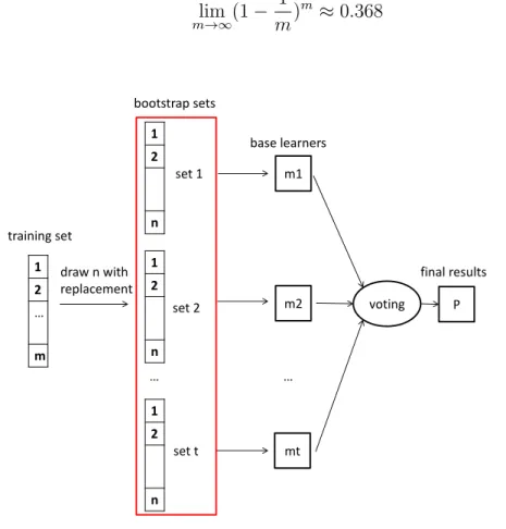
Bagging [5] is the abbreviation of bootstrap aggregating. It is based on bootstrap [13] sampling: given a data set containingmsamples, we take outmsamples with replacement. Some instances appear in this sampling set many times and some instances don’t appear in it. We can do a simple estimate of one instance not appearing in the sampling set: in m

(24)

time sampling, the probability of one instance not taken out is(1−1/m)m_{, the limit is:} lim m→∞(1− 1 m) m_≈₀_.₃₆₈ _(3.4) 1 2 … m 1 2 n 1 2 n 1 2 n training set set 1 set 2 set t draw n with replacement … bootstrap sets voting P base learners final results m1 m2 mt …

Figure 3.1: The frame of bagging

Presently,tsampling set can be generated, thentlearners can be trained based on each sampling set and then combined thesetlearners to final result. All the above is the process of Bagging.

For unsupervised problem, bagging is easy to use because it doesn’t depend on inter-mediate evaluation in which step the label is necessary.

3.2.2 Boosting

(25)

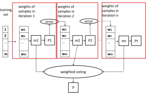
com-Step 1: The base learner assigns equal weight or attention to each observation.

Step 2: According to the performance of former base learner, we pay higher attention to samples which did worse in former base learner. Then, we apply the next base learner.

Step 3: Iterate Step 2 till the number of learner reaches the setting in advance. Next, it combines the outputs from base learners in a certain way.

1 2 … m w1 w2 … wm training set weights of samples in iteration 1 m1 w1 w2 … wm m2 P1 P2 w1 w2 … wm mt Pt error weighted voting P … weights of samples in iteration 2 weights of samples in iteration n error

Figure 3.2: The frame of boosting

All the above is for supervised problem. For unsupervised problem, there is no label for internal validity measures in intermediate steps (Step 2). One commonly used heuristic approach, which is discussed in [1], is to remove outliers in successive iterations in order to build a successively more robust outlier model iteratively. This is a sequential ensemble. The basic idea is that outliers interfere with the creation of a model of normal data, and the removal of points with high outliers scores will be beneficial for the model in the next iteration. It is equivalent that instances with high outliers score in the former learner are assigned with the weight of zero for next iteration. It is not exactly the same as how boosting is understood in the supervised literature, but it is also a sequential method.

(26)

3.3 Bias-Variance Tradeoff

Bias-variance tradeoff is a good explanation of better performance of ensemble learners. The performance of a learning machine on training data set is called “training error”, and the performance on test data set is called “generalization error”. The aim is to minimize the generalization error and ensemble is an important idea to minimize the generalization error. Bias-variance decomposition of generalization error is a good way to explain why ensemble approaches can perform better.

Bias-variance decomposition tries to decompose generalization error: SupposeD is training data set. For test instancex,yD is donated as the label ofxin the training data set

andyis the real label ofx. f(x;D)is the output of modelf which is learned fromDofx. The expected value of modelf inxis :

f(x) = _ED[f(x;D)] (3.5)

The variance due to different dataDis:

var(x) = _ED[(f(x;D)−f(x))2], (3.6)

The intrinsic noise is:

ε2 =_ED[(yD−y)2] (3.7)

The difference of expected output of the model and the real label is donated as bias:

bias2(x) = (f(x)−y)2. (3.8)

(27)

ED[yD]−y= 0. Then, The expected generalization error can be decomposed as below: E(f;D) =_ED[(f(x;D)−yD)2] =_ED[(f(x;D)−f(x) +f(x)−yD)2] =_ED[((f(x;D)−f(x))2] +ED[(f(x)−yD)2] +ED[2(f(x;D)−f(x))(f(x)−yD)] =_ED[((f(x;D)−f(x))2] +ED[(f(x)−yD)2] =_ED[((f(x;D)−f(x))2] +_ED[(f(x)−y+y−yD)2] =_ED[((f(x;D)−f(x))2] +ED[(f(x)−y)2] +ED[(y−yD)2] + 2ED[(f(x)−y)(y−yD)] =_ED[(f(x;D)−f(x))2] + (f(x)−y)2+ED[(y−yD)2] (3.9) That is: E[(f;D)] =bias2(x) +var(x) +ε2 (3.10)

From the equation, we know that generalization error can be decomposed to bias, variance and intrinsic noise. Bias means the deviation between expected value of learning algorithm and real result. Variance means training data set varies results in the learning ability, that is the influence of data perturbation. Intrinsic noise is the lower bound of the generalization error of the current task, that is the difficulty of the task. The bias-variance decomposition shows that generalization error is jointly decided by the ability of algorithm, the sufficiency of the data and the difficulty of the task. Giving the task, to get the better performance of generalization, reducing bias and reducing variances are two approaches (the model fitting data as much as possible, and the influence of data perturbation as low as possible).

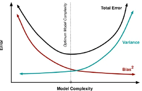
In general, conflicts always exist between reducing bias and variance. It is so called bias-variance dilemma, illustrated in the figure below 3.3. When training is insufficient, the ability of learning machine is not strong enough, data perturbation would not have significant influence on the learning machine and therefore bias leads to generalization

(28)

Figure 3.3: bias-variance dilemma

error. With the degree of training grows, learning machine becomes stronger and data perturbation can be learned gradually, then variance is the dominant factor. After enough training, learning machine becomes strong enough and any tiny perturbation of training data will show effect on the learning machine. Overfitting would appear if the machine learns the non-global characteristic of training data.

Ensemble is a way that combines different models in order to ensure that the bias-variance tradeoff is optimized. This is achieved in two ways: reducing bias and reducing variance [15]. Bagging focuses on reducing variance: since each base learner generated in bagging is identically distributed (i.d.), the expectation of the average oft base learners is the same as the expectation of any one of them:

E(1 t t X i=1 Xi) = E(Xi) (3.11)

(29)

(identically distributed) with positive pairwise correlationρ, the variance of the average is: V ar(1 t t X i=1 Xi) = 1 t2{E[( t X i=1 Xi)2]−E[ t X i=1 Xi]2} =ρσ2+1−ρ t σ 2 (3.12)

If the variables are completely independent, thenρis zero and the first item in the equation is zero. Then, we can find that variance is reduced obviously. If the variables are same, thenρis one and the second item is zero. Then, the variance keeps constant. For bagging method, the training sets of each base learner are always overlapped but not the same, so

ρis between zero and one, then the variance should be reduced. For boosting method, the base learners are strongly dependent, soρis close to one, then variance will not be reduced obviously.

For unsupervised problem, there is no ground truth for training data, so the intrinsic error is missing. But unknown ground truth does exist. In the progress of aforementioned compu-tation , there is no need forf(x;D)to be computed. In conclusion, bias-variance tradeoff can generalize easily from supervised approaches to unsupervised approaches.

3.4 Strategy of diversity

The core of ensemble is how to generate “good and diverse” base learners. The general idea is to introduce randomness. The common method is creating some perturbation of training set, features, parameters of algorithms respectively.

3.4.1 Training data perturbation

The main idea is to obtain different subsets from the initial training data, then build base learners with the subsets respectively. Sampling is the common method such as bootstrap

(30)

in bagging. This way is simple and effective for some algorithms which are sensitive to training data. For some stable base learner, which are not sensitive to training data, other perturbation should be introduced.

3.4.2 Feature perturbation

Various subspace provides virous views of training data and it is obvious that learners trained with different subspace will be diverse. For feature perturbation, subsets only con-tain some features of the initial training data.

For training data with redundant attributes, training base learners in subspace will not only produce diverse individual ones but also save time due to feature reducing. Under this condition, due to redundant attributes, base learners would not be too bad. But if initial training data contains too few features or redundant features are very few, feature perturbation is not a good choice.

3.4.3 Parameters Perturbation

There are always some parameters to be set for base learners, such as k in K-Nearest-Neighbors algorithm. Virous base learners can be trained with different parameters. It is worth noting that, when individual learners is trained, we always try several groups of parameters and then select the best ones. So, different learners have been trained already. It selects only the best one, but ensemble methods combine all of these learners together. Therefore, the costs of ensemble methods are not too larger than those of the individual learners.

(31)

Chapter 4: Experiments and Results

4.1 Evaluation Method

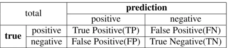
Outlier detection is a two-class problem, in which the outcomes are labeled either as posi-tive (p) or negaposi-tive (n). There are four possible outcomes. If the outcome from a prediction is p and the actual value is also p, then it is called a true positive (TP); however if the actual value is n then it is said to be a false positive (FP). Conversely, a true negative (TN) has occurred when both the prediction outcome and the actual value are n, and false negative (FN) is when the prediction outcome is n while the actual value is p. The four outcomes can be formulated in a2×2confusion matrix as follows.

Table 4.1: confusion matrix

total prediction

positive negative

true positive True Positive(TP) False Positive(FN)

negative False Positive(FP) True Negative(TN)

The confusion matrix can derive several metrics. Precision and Recall are defined as follows:

P recision= T P

T P +F P (4.1)

Recall= T P

(32)

Ideally, we hope T P and T N are the same with the number of true positive and negative instances, and thenF N andF P would be zero. In practice, if we want to obtain moreT P through increasing the number of predict positive ones, recall will be high and precision will be low. On the other hand, if we just pick up the most likely instances, some true positive ones would be missing, then recall will be low and precision will be high. In other words, precision and recall are always in conflict: when precision becomes higher, recall would become lower and vice versa.

We can sort instances according to their outlier score (possibility). Set threshold of positive ones in this order one by one, then precision-recall curve can be obtained. For an ideal learning machine, precision can keep well with recall grows, as shown in the figure below. The bottom left area is the average precision, obviously the maximum is 1. The higher the area is, the better the learning machine is.

0 0.2 0.4 0.6 0.8 1 0.2 0.4 0.6 0.8 1

Recall

Precision

Figure 4.1: Precision-Recall Curve

(33)

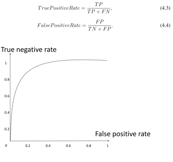
ob-then consider samples as positive ones one by one to get two values as vertical and hori-zontal coordinates. Different from Precision Recall curve, the vertical axis is True Positive Rate, and horizontal axis is False Positive Rate. They are defined as follows with signs in Figure4.2: T rueP ositiveRate= T P T P +F N, (4.3) F alseP ositiveRate= F P T N+F P. (4.4) 0 0.2 0.4 0.6 0.8 1 0.2 0.4 0.6 0.8 1

False positive rate

True negative rate

Figure 4.2: ROC Curve

Similar with Precision Recall curve, if ROC curve of one learner is completely “sur-rounded” by another curve of learner, we can determine that the performance of latter learner is better than that of the former learner. If two curves are crossed, the area under the curve (AUC) can then be the criterion (the larger, the better). For outlier detection, positive instances are few, so we pay more attention to the performance with low false positive rate. Here, the area under the curve and being the left part of false positive rate being 0.1 is considered, which is signed AUC0.1. Similarly, the larger the area is, the better the learner

(34)

is.

4.2 Data set Description and Experiment Environment

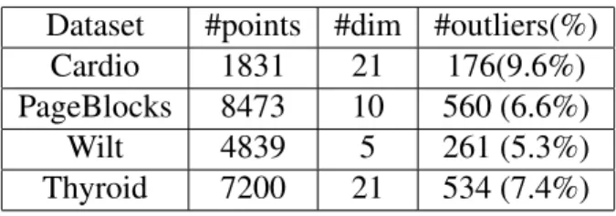
We used four data sets from UCI machine learning repository [23]. A brief description is provided here:

The Cardiotocography (Cardio) data set contains measurements taken from fetal heart rate signals. The classes in the data set are normal, suspect, pathologic and the normal

class forms the inliers while the pathologicclass forms outlier class. The suspectclass is discarded. The PageBlock data set are block information of documents. The data sets are divided into 5 classes: text, horizontal line, picture, vertical line and graphic. Thetextclass forms inlier class and others form outlier class. The wilt is high-resolution remote sensing data set. Diseased treesclass forms outlier class andthe other land coverclass forms inlier class. The thyroid data set contains data of thyroid disease. Similar with Cardio data,

normalclass forms the inliers while the hyperfunctionclass forms outlier class. Refer to

table for details of data sets.

Table 4.2: summary of data sets

Dataset #points #dim #outliers(%) Cardio 1831 21 176(9.6%) PageBlocks 8473 10 560 (6.6%) Wilt 4839 5 261 (5.3%) Thyroid 7200 21 534 (7.4%)

(35)

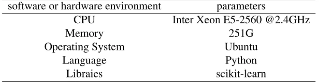
Table 4.3: software and hardware environment of experiments

software or hardware environment parameters

CPU Inter Xeon E5-2560 @2.4GHz

Memory 251G

Operating System Ubuntu

Language Python

Libraies scikit-learn

4.3 Experiments setup and results

We set up groups of experiments to prove relative effectiveness of ensemble methods and bagging and boosting can improve performance of base learners in outlier detection prob-lem.

4.3.1 Supervised Ensemble

Decision Tree and SVM algorithms are set as base learners.

For bagging method, 100 trials of base learners are used with 70 percent bootstrap samples. The outlier scores are also normalized in each trial then average of the 100 results is set as the ultimate score.

For boosting method, 100 iterations are used. Sample weights are changed in each iteration and the 100 learners are weighted according to their performance.

Stratified k fold cross validation are used. The proportion of outliers and inliers are kept constant in Stratified method [27].

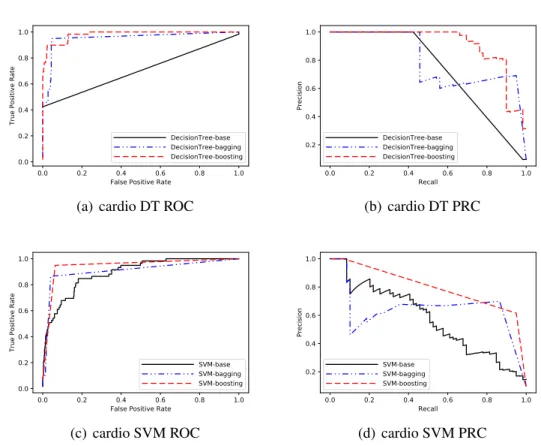
From Figure 4.3, Figure 4.4, Figure 4.5, Figure 4.6 and the numbers in table, we can conclude that bagging and boosting methods perform better than their corresponding base algorithms in these four data sets. Bagging method sometimes gets results close to base learners, such as Figure4.5(c)and Figure4.6(d). From these two figures, we can see that base learners don’t perform well. According to theoretical analysis in above chapter, bagging method need relatively strong base learners. By contrast, boosting can be effective

(36)

0.0 0.2 0.4 0.6 0.8 1.0 False Positive Rate

0.0 0.2 0.4 0.6 0.8 1.0

True Positive Rate

DecisionTree-base DecisionTree-bagging DecisionTree-boosting

(a) cardio DT ROC

0.0 0.2 0.4 0.6 0.8 1.0 Recall 0.2 0.4 0.6 0.8 1.0 Precision DecisionTree-base DecisionTree-bagging DecisionTree-boosting (b) cardio DT PRC 0.0 0.2 0.4 0.6 0.8 1.0

False Positive Rate 0.0 0.2 0.4 0.6 0.8 1.0

True Positive Rate

SVM-base SVM-bagging SVM-boosting (c) cardio SVM ROC 0.0 0.2 0.4 0.6 0.8 1.0 Recall 0.2 0.4 0.6 0.8 1.0 Precision SVM-base SVM-bagging SVM-boosting (d) cardio SVM PRC Figure 4.3: supervised results of cardio dataset

with weak base learners.

The AUC value for ROC curve and average precision(AP) for each algorithm and each data set is shown in the table4.4

(37)

0.0 0.2 0.4 0.6 0.8 1.0

True Positive Rate

(a) pageblock DT ROC

0.0 0.2 0.4 0.6 0.8 1.0 Recall 0.2 0.4 0.6 0.8 1.0 Precision DecisionTree-base DecisionTree-bagging DecisionTree-boosting (b) pageblock DT PRC 0.0 0.2 0.4 0.6 0.8 1.0

True Positive Rate

SVM-base SVM-bagging SVM-boosting (c) pageblock SVM ROC 0.0 0.2 0.4 0.6 0.8 1.0 Recall 0.2 0.4 0.6 0.8 1.0 Precision SVM-base SVM-bagging SVM-boosting (d) pageblock SVM PRC Figure 4.4: supervised results of pageblock dataset

0.0 0.2 0.4 0.6 0.8 1.0

True Positive Rate

(a) wilt DT ROC

0.0 0.2 0.4 0.6 0.8 1.0 Recall 0.0 0.2 0.4 0.6 0.8 1.0 Precision DecisionTree-base DecisionTree-bagging DecisionTree-boosting (b) wilt DT PRC 0.0 0.2 0.4 0.6 0.8 1.0

True Positive Rate

SVM-base SVM-bagging SVM-boosting (c) wilt SVM ROC 0.0 0.2 0.4 0.6 0.8 1.0 Recall 0.0 0.2 0.4 0.6 0.8 1.0 Precision SVM-base SVM-bagging SVM-boosting (d) wilt SVM PRC Figure 4.5: supervised results of wilt dataset

(38)

0.0 0.2 0.4 0.6 0.8 1.0

True Positive Rate

(a) thyroid DT ROC

0.0 0.2 0.4 0.6 0.8 1.0 Recall 0.88 0.90 0.92 0.94 0.96 0.98 1.00 Precision DecisionTree-base DecisionTree-bagging DecisionTree-boosting (b) thyroid DT PRC 0.0 0.2 0.4 0.6 0.8 1.0

True Positive Rate

SVM-base SVM-bagging SVM-boosting (c) thyroid SVM ROC 0.0 0.2 0.4 0.6 0.8 1.0 Recall 0.2 0.4 0.6 0.8 1.0 Precision SVM-base SVM-bagging SVM-boosting (d) thyroid SVM PRC Figure 4.6: supervised results of thyroid dataset

Table 4.4: supervised ensemble results

Cardio PageBlock Wilt Thyroid Algorithm ROC AP ROC AP ROC AP ROC AP

AUC AUC AUC AUC

DT-base 0.70 0.73 0.91 0.88 0.74 0.43 0.99 0.97 DT-bagging 0.95 0.79 0.98 0.95 0.90 0.43 0.99 0.98 DT-boosting 0.98 0.91 0.99 0.96 0.98 0.78 0.99 0.99 SVM-base 0.89 0.57 0.91 0.63 0.75 0.11 0.87 0.54 SVM-bagging 0.91 0.65 0.99 0.90 0.75 0.10 0.86 0.49 SVM-boosting 0.95 0.80 0.95 0.90 0.82 0.16 0.87 0.58

(39)

4.3.2 Unsupervised Ensemble

Six algorithms referred in Section 2.2 are used as base learner. kis set to 20.

For Bagging, three strategies of diversity (diversity of samples, diversity of features and diversity of model parameters which are referred in section 3.4) have been used. Specif-ically, they are bootstrap of 70 percent samples, bootstrap of 70 percent features and 30k

values (from10 to300 with interval of 10). For Boosting, how it works in unsupervised problem is discussed in section 3.2. 0.5 percent samples which are suspected to be outliers would be discarded in each iteration. We use 50 iterations. Results for different data set are shown below.

Figures show the comparison of base algorithms and the three strategies of bagging and boosting. In Figure4.7, bagging of samples and bagging of features perform almost the same with base learners, not outstanding. The small scale and limit of feature attributes of the data set may be the reason. Bagging ofkshows the obvious enhancement than base learners and boosting sometimes seems even better than bagging of k. In Figure 4.8, the observation is almost the same. In Figure4.9 and Figure4.10, precision and recall curves show that the base learner is weak, so bagging or boosting seems not improving the results. But in ROC curves, bagging and boosting methods also are the better ones.

(40)

0.0 0.2 0.4 0.6 0.8 1.0

True Positive Rate knn_{knn_bagging_sample}

knn_bagging_feature knn_bagging_k knn_boosting

(a) cardio knn ROC

0.0 0.2 0.4 0.6 0.8 1.0 Recall 0.2 0.4 0.6 0.8 1.0 Precision knn knn_bagging_sample knn_bagging_feature knn_bagging_k knn_boosting (b) cardio knn PRC 0.0 0.2 0.4 0.6 0.8 1.0

True Positive Rate knnw_{knnw_bagging_sample}

knnw_bagging_feature knnw_bagging_k knnw_boosting (c) cardio knnw ROC 0.0 0.2 0.4 0.6 0.8 1.0 Recall 0.2 0.4 0.6 0.8 1.0 Precision knnw knnw_bagging_sample knnw_bagging_feature knnw_bagging_k knnw_boosting (d) cardio knnw PRC 0.0 0.2 0.4 0.6 0.8 1.0

True Positive Rate odin_{odin_bagging_sample}

odin_bagging_feature odin_bagging_k odin_boosting

(e) cardio odin ROC

0.0 0.2 0.4 0.6 0.8 1.0 Recall 0.2 0.4 0.6 0.8 1.0 Precision odin odin_bagging_sample odin_bagging_feature odin_bagging_k odin_boosting (f) cardio odin PRC

(41)

0.0 0.2 0.4 0.6 0.8 1.0

True Positive Rate lof_{lof_bagging_sample}

lof_bagging_feature lof_bagging_k lof_boosting

(g) cardio lof ROC

0.0 0.2 0.4 0.6 0.8 1.0 Recall 0.2 0.3 0.4 0.5 0.6 0.7 0.8 0.9 1.0 Precisioin lof lof_bagging_sample lof_bagging_feature lof_bagging_k lof_boosting (h) cardio lof PRC 0.0 0.2 0.4 0.6 0.8 1.0

True Positive Rate slof_{slof_bagging_sample}

slof_bagging_feature slof_bagging_k slof_boosting

(i) cardio slof ROC

0.0 0.2 0.4 0.6 0.8 1.0 Recall 0.2 0.4 0.6 0.8 1.0 Precision slof slof_bagging_sample slof_bagging_feature slof_bagging_k slof_boosting (j) cardio slof PRC 0.0 0.2 0.4 0.6 0.8 1.0

True Positive Rate inflo_{inflo_bagging_sample}

inflo_bagging_feature inflo_bagging_k inflo_boosting

(k) cardio inflo ROC

0.0 0.2 0.4 0.6 0.8 1.0 Recall 0.2 0.4 0.6 0.8 1.0 Precision inflo inflo_bagging_sample inflo_bagging_feature inflo_bagging_k inflo_boosting (l) cardio inflo PRC

(42)

0.0 0.2 0.4 0.6 0.8 1.0

(a) pageblock knn ROC

0.0 0.2 0.4 0.6 0.8 1.0 Recall 0.0 0.2 0.4 0.6 0.8 1.0 Precision knn knn_bagging_sample knn_bagging_feature knn_bagging_k knn_boosting (b) pageblock knn PRC 0.0 0.2 0.4 0.6 0.8 1.0

knnw_bagging_feature knnw_bagging_k knnw_boosting (c) pageblock knnw ROC 0.0 0.2 0.4 0.6 0.8 1.0 Recall 0.0 0.2 0.4 0.6 0.8 1.0 Precision knnw knnw_bagging_sample knnw_bagging_feature knnw_bagging_k knnw_boosting (d) pageblock knnw PRC 0.0 0.2 0.4 0.6 0.8 1.0

(e) pageblock odin ROC

0.0 0.2 0.4 0.6 0.8 1.0 Recall 0.0 0.2 0.4 0.6 0.8 1.0 Precision odin odin_bagging_sample odin_bagging_feature odin_bagging_k odin_boosting (f) pageblock odin PRC

(43)

0.0 0.2 0.4 0.6 0.8 1.0

(g) pageblock lof ROC

0.0 0.2 0.4 0.6 0.8 1.0 Recall 0.0 0.2 0.4 0.6 0.8 1.0 Precisioin lof lof_bagging_sample lof_bagging_feature lof_bagging_k lof_boosting (h) pageblock lof PRC 0.0 0.2 0.4 0.6 0.8 1.0

(i) pageblock slof ROC

0.0 0.2 0.4 0.6 0.8 1.0 Recall 0.0 0.2 0.4 0.6 0.8 1.0 Precision slof slof_bagging_sample slof_bagging_feature slof_bagging_k slof_boosting (j) pageblock slof PRC 0.0 0.2 0.4 0.6 0.8 1.0

(k) pageblock inflo ROC

0.0 0.2 0.4 0.6 0.8 1.0 Recall 0.0 0.2 0.4 0.6 0.8 1.0 Precision knn knn_bagging_sample knn_bagging_feature knn_bagging_k knn_boosting (l) pageblock inflo PRC

(44)

0.0 0.2 0.4 0.6 0.8 1.0

(a) wilt knn ROC

0.0 0.2 0.4 0.6 0.8 1.0 Recall 0.000 0.025 0.050 0.075 0.100 0.125 0.150 0.175 0.200 Precision knn knn_bagging_sample knn_bagging_feature knn_bagging_k knn_boosting (b) wilt knn PRC 0.0 0.2 0.4 0.6 0.8 1.0

knnw_bagging_feature knnw_bagging_k knnw_boosting (c) wilt knnw ROC 0.0 0.2 0.4 0.6 0.8 1.0 Recall 0.000 0.025 0.050 0.075 0.100 0.125 0.150 0.175 0.200 Precision knnw knnw_bagging_sample knnw_bagging_feature knnw_bagging_k knnw_boosting (d) wilt knnw PRC 0.0 0.2 0.4 0.6 0.8 1.0

(e) wilt odin ROC

0.0 0.2 0.4 0.6 0.8 1.0 Recall 0.000 0.025 0.050 0.075 0.100 0.125 0.150 0.175 0.200 Precision odin odin_bagging_sample odin_bagging_feature odin_bagging_k odin_boosting (f) wilt odin PRC

(45)

0.0 0.2 0.4 0.6 0.8 1.0

(g) wilt lof ROC

0.0 0.2 0.4 0.6 0.8 1.0 Recall 0.000 0.025 0.050 0.075 0.100 0.125 0.150 0.175 0.200 Precisioin lof lof_bagging_sample lof_bagging_feature lof_bagging_k lof_boosting (h) wilt lof PRC 0.0 0.2 0.4 0.6 0.8 1.0

(i) wilt slof ROC

0.0 0.2 0.4 0.6 0.8 1.0 Recall 0.000 0.025 0.050 0.075 0.100 0.125 0.150 0.175 0.200 Precision slof slof_bagging_sample slof_bagging_feature slof_bagging_k slof_boosting (j) wilt slof PRC 0.0 0.2 0.4 0.6 0.8 1.0

(k) wilt inflo ROC

0.0 0.2 0.4 0.6 0.8 1.0 Recall 0.000 0.025 0.050 0.075 0.100 0.125 0.150 0.175 0.200 Precision knn knn_bagging_sample knn_bagging_feature knn_bagging_k knn_boosting (l) wilt inflo PRC

(46)

0.0 0.2 0.4 0.6 0.8 1.0

(a) thyroid knn ROC

0.0 0.2 0.4 0.6 0.8 1.0 Recall 0.000 0.025 0.050 0.075 0.100 0.125 0.150 0.175 0.200 Precision knn knn_bagging_sample knn_bagging_feature knn_bagging_k knn_boosting (b) thyroid knn PRC 0.0 0.2 0.4 0.6 0.8 1.0

knnw_bagging_feature knnw_bagging_k knnw_boosting (c) thyroid knnw ROC 0.0 0.2 0.4 0.6 0.8 1.0 Recall 0.000 0.025 0.050 0.075 0.100 0.125 0.150 0.175 0.200 Precision knnw knnw_bagging_sample knnw_bagging_feature knnw_bagging_k knnw_boosting (d) thyroid knnw PRC 0.0 0.2 0.4 0.6 0.8 1.0

(e) thyroid odin ROC

0.0 0.2 0.4 0.6 0.8 1.0 Recall 0.00 0.05 0.10 0.15 0.20 0.25 0.30 0.35 0.40 Precision odin odin_bagging_sample odin_bagging_feature odin_bagging_k odin_boosting (f) thyroid odin PRC

(47)

0.0 0.2 0.4 0.6 0.8 1.0

(g) wilt lof ROC

0.0 0.2 0.4 0.6 0.8 1.0 Recall 0.000 0.025 0.050 0.075 0.100 0.125 0.150 0.175 0.200 Precisioin lof lof_bagging_sample lof_bagging_feature lof_bagging_k lof_boosting (h) wilt lof PRC 0.0 0.2 0.4 0.6 0.8 1.0

(i) wilt slof ROC

0.0 0.2 0.4 0.6 0.8 1.0 Recall 0.0 0.2 0.4 0.6 0.8 1.0 Precision slof slof_bagging_sample slof_bagging_feature slof_bagging_k slof_boosting (j) wilt slof PRC 0.0 0.2 0.4 0.6 0.8 1.0

(k) wilt inflo ROC

0.0 0.2 0.4 0.6 0.8 1.0 Recall 0.000 0.025 0.050 0.075 0.100 0.125 0.150 0.175 0.200 Precision knn knn_bagging_sample knn_bagging_feature knn_bagging_k knn_boosting (l) wilt inflo PRC

(48)

The tables below show the ensemble results based on different base learners.

Table 4.5: unsupervised ensemble results based on knn

AUC AUC AUC AUC

knn 0.89 0.47 0.66 0.22 0.59 0.07 0.81 0.06 knn bagging samples 0.91 0.51 0.66 0.22 0.63 0.07 0.78 0.05 knn bagging features 0.90 0.45 0.64 0.20 0.64 0.07 0.84 0.07 knn bagging k 0.95 0.62 0.66 0.21 0.64 0.07 0.66 0.03 knn boosting 0.93 0.57 0.67 0.22 0.66 0.08 0.81 0.06

Table 4.6: unsupervised ensemble results based on knnw

AUC AUC AUC AUC

knnw 0.89 0.39 0.66 0.23 0.76 0.09 0.72 0.04 knnw bagging samples 0.91 0.43 0.66 0.22 0.75 0.09 0.70 0.04 knnw bagging features 0.90 0.39 0.64 0.21 0.68 0.07 0.75 0.04 knnw bagging k 0.95 0.56 0.66 0.22 0.69 0.08 0.70 0.04 knnw boosting 0.93 0.58 0.67 0.22 0.70 0.08 0.65 0.03

Table 4.7: unsupervised ensemble results based on odin

AUC AUC AUC AUC

odin 0.83 0.29 0.89 0.18 0.78 0.14 0.72 0.04 odin bagging samples 0.87 0.34 0.88 0.20 0.75 0.12 0.70 0.04 odin bagging features 0.83 0.28 0.90 0.30 0.73 0.09 0.75 0.04 odin bagging k 0.83 0.29 0.89 0.18 0.78 0.14 0.70 0.04 odin boosting 0.83 0.37 0.89 0.22 0.71 0.08 0.65 0.03

(49)

Table 4.8: unsupervised ensemble results based on lof

AUC AUC AUC AUC

lof 0.91 0.43 0.88 0.25 0.75 0.11 0.64 0.04 lof bagging samples 0.94 0.60 0.68 0.19 0.56 0.06 0.64 0.03 lof bagging features 0.91 0.38 0.90 0.25 0.74 0.09 0.53 0.03 lof bagging k 0.94 0.51 0.90 0.26 0.74 0.09 0.66 0.04 lof boosting 0.95 0.65 0.66 0.19 0.67 0.07 0.65 0.04

Table 4.9: unsupervised ensemble results based on slof

AUC AUC AUC AUC

slof 0.86 0.37 0.87 0.22 0.77 0.11 0.72 0.05 slof bagging samples 0.93 0.55 0.66 0.22 0.57 0.07 0.67 0.04 slof bagging features 0.86 0.33 0.89 0.20 0.73 0.09 0.56 0.03 slof bagging k 0.96 0.70 0.88 0.28 0.69 0.08 0.71 0.05 slof boosting 0.96 0.68 0.68 0.22 0.70 0.08 0.74 0.04

Table 4.10: unsupervised ensemble results based on inflo

AUC AUC AUC AUC

inflo 0.87 0.40 0.85 0.23 0.78 0.15 0.69 0.04 inflo bagging samples 0.93 0.56 0.64 0.24 0.93 0.12 0.65 0.04 inflo bagging features 0.86 0.38 0.86 0.19 0.77 0.11 0.55 0.03 inflo bagging k 0.96 0.75 0.88 0.25 0.70 0.15 0.67 0.03 inflo boosting 0.96 0.71 0.68 0.23 0.71 0.20 0.63 0.05

(50)

Conclusion

In this thesis, we demonstrate the effectiveness of ensemble methods for outlier detection. First, we review some algorithms for class imbalance problem in both supervised and un-supervised problems. Next, we present the ensemble frame and some typical methods: bagging and boosting. We also analyze the reason of the enhanced performance of en-semble method in the view of bias-variance tradeoff. Next, the strategies of increasing the diversity of base learners are introduced. Finally, experiment results in various data sets show that bagging and boosting are effective in outlier detection based on various base learners.

(51)

Bibliography

[1] Charu C Aggarwal. Outlier ensembles: position paper. ACM SIGKDD Explorations

Newsletter, 14(2):49–58, 2013.

[2] Charu C Aggarwal and Philip S Yu. Outlier detection for high dimensional data. In

ACM Sigmod Record, volume 30, pages 37–46. ACM, 2001.

[3] Fabrizio Angiulli and Clara Pizzuti. Fast outlier detection in high dimensional spaces.

In European Conference on Principles of Data Mining and Knowledge Discovery,

pages 15–27. Springer, 2002.

[4] Stephen D Bay and Mark Schwabacher. Mining distance-based outliers in near linear time with randomization and a simple pruning rule. InProceedings of the ninth ACM

SIGKDD international conference on Knowledge discovery and data mining, pages

29–38. ACM, 2003.

[5] Leo Breiman. Bagging predictors. Machine learning, 24(2):123–140, 1996.

[6] Leo Breiman. Random forests. Machine learning, 45(1):5–32, 2001.

[7] Markus M Breunig, Hans-Peter Kriegel, Raymond T Ng, and J¨org Sander. Lof: iden-tifying density-based local outliers. InACM sigmod record, volume 29, pages 93–104. ACM, 2000.

(52)

[8] Varun Chandola, Arindam Banerjee, and Vipin Kumar. Anomaly detection: A survey.

ACM computing surveys (CSUR), 41(3):15, 2009.

[9] Bertrand Clarke. Comparing bayes model averaging and stacking when model approximation error cannot be ignored. Journal of Machine Learning Research, 4(Oct):683–712, 2003.

[10] Corinna Cortes and Vladimir Vapnik. Support vector machine. Machine learning, 20(3):273–297, 1995.

[11] Pedro Domingos. Bayesian averaging of classifiers and the overfitting problem. In

ICML, volume 2000, pages 223–230, 2000.

[12] Saso Dˇzeroski and Bernard ˇZenko. Is combining classifiers with stacking better than selecting the best one? Machine learning, 54(3):255–273, 2004.

[13] Bradley Efron.The jackknife, the bootstrap and other resampling plans. SIAM, 1982.

[14] Yoav Freund and Robert E Schapire. A desicion-theoretic generalization of on-line learning and an application to boosting. In European conference on computational

learning theory, pages 23–37. Springer, 1995.

[15] Jerome Friedman, Trevor Hastie, and Robert Tibshirani. The elements of statistical

learning, volume 1. Springer series in statistics New York, 2001.

[16] Ville Hautamaki, Ismo Karkkainen, and Pasi Franti. Outlier detection using k-nearest neighbour graph. InPattern Recognition, 2004. ICPR 2004. Proceedings of the 17th

International Conference on, volume 3, pages 430–433. IEEE, 2004.

[17] Wen Jin, Anthony KH Tung, and Jiawei Han. Mining top-n local outliers in large databases. InProceedings of the seventh ACM SIGKDD international conference on

(53)

[18] Wen Jin, Anthony KH Tung, Jiawei Han, and Wei Wang. Ranking outliers using sym-metric neighborhood relationship. InPacific-Asia Conference on Knowledge

Discov-ery and Data Mining, pages 577–593. Springer, 2006.

[19] Theodore Johnson, Ivy Kwok, and Raymond T Ng. Fast computation of 2-dimensional depth contours. InKDD, pages 224–228, 1998.

[20] Edwin M Knorr and Raymond T Ng. Finding intensional knowledge of distance-based outliers. InVLDB, volume 99, pages 211–222, 1999.

[21] Edwin M Knox and Raymond T Ng. Algorithms for mining distancebased outliers in large datasets. InProceedings of the International Conference on Very Large Data

Bases, pages 392–403. Citeseer, 1998.

[22] Ron Kohavi. Scaling up the accuracy of naive-bayes classifiers: A decision-tree hy-brid. InKDD, volume 96, pages 202–207, 1996.

[23] M. Lichman. UCI machine learning repository, 2013.

[24] Mehryar Mohri, Afshin Rostamizadeh, and Ameet Talwalkar.Foundations of machine

learning. MIT press, 2012.

[25] Spiros Papadimitriou, Hiroyuki Kitagawa, Phillip B Gibbons, and Christos Faloutsos. Loci: Fast outlier detection using the local correlation integral. InData Engineering,

2003. Proceedings. 19th International Conference on, pages 315–326. IEEE, 2003.

[26] Sridhar Ramaswamy, Rajeev Rastogi, and Kyuseok Shim. Efficient algorithms for mining outliers from large data sets. InACM Sigmod Record, volume 29, pages 427– 438. ACM, 2000.

[27] Payam Refaeilzadeh, Lei Tang, and Huan Liu. Cross-validation. InEncyclopedia of

(54)

[28] Erich Schubert, Arthur Zimek, and Hans-Peter Kriegel. Local outlier detection re-considered: a generalized view on locality with applications to spatial, video, and network outlier detection. Data Mining and Knowledge Discovery, 28(1):190–237, 2014.

[29] Padhraic Smyth and David Wolpert. Linearly combining density estimators via

stack-ing. Machine Learning, 36(1-2):59–83, 1999.

A Comparative Study of Bagging and Boosting of Supervised and Unsupervised Classifiers for Outliers Detection

CORE Scholar

CORE Scholar

A Comparative Study of Bagging and Boosting of Supervised and

A Comparative Study of Bagging and Boosting of Supervised and

Unsupervised Classifiers for Outliers Detection

Unsupervised Classifiers for Outliers Detection

A COMPARATIVE STUDY OF BAGGING AND

BOOSTING OF SUPERVISED AND

UNSUPERVISED CLASSIFIERS FOR

OUTLIERS DETECTION

A thesis submitted in partial fulfillment

of the requirements for the degree of

Master of Science in Electrical Engineering

by

YUE DANG

B.E, University of Electronic Science and Technology of China, 2011

2017

Contents

List of Figures

List of Tables

Chapter 1: Introduction

1.1

Problem Description

1.2

Motivation

1.3

Thesis Outline

Chapter 2: Basic Algorithms

2.1

Supervised Approach

2.1.1

Cost-sensitive Decision Tree

2.1.2

Cost-sensitive Support Vector Machine

2.2

Unsupervised Approach

2.2.1

Distance Based Approaches

2.2.2

Density Based Approach

Chapter 3: Ensemble Learning

3.1

Frame of Ensemble Learning

3.2

Bagging and Boosting

3.2.1

Bagging

3.2.2

Boosting

3.3

Bias-Variance Tradeoff

3.4

Strategy of diversity

3.4.1

Training data perturbation

3.4.2

Feature perturbation

3.4.3

Parameters Perturbation

Chapter 4: Experiments and Results

4.1

Evaluation Method

Recall

Precision

False positive rate

True negative rate

4.2

Data set Description and Experiment Environment

4.3

Experiments setup and results

4.3.1

Supervised Ensemble

4.3.2

Unsupervised Ensemble

Conclusion

Bibliography