Title Content-aware partial compression for textual big data analysis in Hadoop
Author(s) Dong, Dapeng; Herbert, John
Publication date 2017-06-29
Original citation Dong, D. and Herbert, J. (2017) 'Content-aware Partial Compression for
Textual Big Data Analysis in Hadoop', IEEE Transactions on Big Data, In Press, doi: 10.1109/TBDATA.2017.2721431
Type of publication Article (peer-reviewed)
Link to publisher's
version http://dx.doi.org/10.1109/TBDATA.2017.2721431Access to the full text of the published version may require a subscription.
Rights © 2017 IEEE. Personal use of this material is permitted. Permission
from IEEE must be obtained for all other uses, in any current or future media, including reprinting/republishing this material for advertising or promotional purposes, creating new collective works, for resale or redistribution to servers or lists, or reuse of any copyrighted component of this work in other works.
Item downloaded
from http://hdl.handle.net/10468/5452
Downloaded on 2020-07-06T14:31:29Z
Content-aware Partial Compression for Textual
Big Data Analysis in Hadoop
Dapeng Dong,
Member, IEEE
and John Herbert,
Member, IEEE
Abstract—A substantial amount of information in companies and on the Internet is present in the form of text. The value of this semi-structured and unstructured data has been widely acknowledged, with consequent scientific and commercial exploitation. The ever-increasing data production, however, pushes data analytic platforms to their limit. Compression as an effective means to reduce data size has been employed by many emerging data analytic platforms, whom the main purpose of data compression is to save storage space and reduce data transmission cost over the network. Since general purpose compression methods endeavour to achieve higher compression ratios by leveraging data transformation techniques and contextual data, this context-dependency forces the access to the compressed data to be sequential. Processing such compressed data in parallel, such as desirable in a distributed environment, is extremely challenging. This work proposes techniques for more efficient textual big data analysis with an emphasis on content-aware compression schemes suitable for the Hadoop analytic platform. The compression schemes have been evaluated for a number of standard MapReduce analysis tasks using a collection of public and private real-world datasets. In comparison with existing solutions, they have shown substantial improvement in performance and significant reduction in system resource requirements.
Index Terms—Big Data, Compression, MapReduce, Distributed File System.
F
1
I
NTRODUCTIONB
IGdata is now at the frontier of research, innovation andbusiness. The real-world value of big data is evident in a wide range of applications as demonstrated by successful examples including banking [1], healthcare [2], education [3], government [4] and social science [5].
As a valuable asset, data is constantly being collected and accumulated from almost all aspects of life. The term
datafication [6] was coined to capture this phenomenon. It
is predicted that the globaldataficationprocess will generate
44 zetabytes of data by 2020 compared to 4.4 zetabytes in 2013 [7]. It should also be noted that a substantial amount of data being collected is semi-structured or unstructured [8], primarily in text format [9]. The sheer volume of data and the aggressive speed of data growth present major challenges to all aspects of big data analysis from analytic platforms to scalable algorithms. In order to deal with the challenges brought by big data, there is very active ongo-ing development of new tools, algorithms, computational frameworks, analytic platforms and deployment strategies. Current big data analyssi optimization focuses on scaling up/out analytic platforms [10] [11] and using approxima-tion algorithms [12] [13].
Another optimization, complementary to those other optimizations would be to reduce the size of the source data through compression, and support the direct use of the compressed data in analysis. This aspect of leveraging compression for big data analysis in distributed environ-ments has not been given much attention. On current an-alytic platforms, such as Hadoop, the purpose of compres-sion is to reduce data size in order to save storage space
• D. Dong is with the Boole Centre for Research in Informatics, University
College Cork, Ireland. E-mail: [email protected]
• J. Herbert is with Department of Computer Science, University College
Cork, Ireland.E-mail: [email protected]
and lower the data transmission cost over the network. Currently, compressed data cannot be directly involved in MapReduce-based computation. In order to carry out an analysis, the compressed data must firstly be decom-pressed fully in a sequential manner – sequential due to the fact that modern compression schemes often employ data transformation and/or contextualization techniques which create strong dependencies within the compressed data. The decompression process also requires the under-lying storage system to maintain sufficient free space for holding the decompressed data. Additionally, depending on the compression algorithms, decompression speed varies greatly. This can delay considerably the delivery of analysis results when the data volume is large. It should also be noted that previous research has identified that the Input and Output (I/O) system (including both disk I/O and network I/O) is often the bottleneck for data-centric analysis in a distributed environment [14] [15]. The network I/O efficiency can be improved by compressing the intermediate data that is going to be transmitted over the network. The disk I/O efficiency can also be improved if the compressed data can be decompressed in parallel in memory as data is being consumed at each computational node of Hadoop (parallel decompression in memory). In this way, the total decompression time can be reduced in proportion to the number of parallel processes. The data loading time can thus be kept to a minimum, and the use of extra storage space can be avoided.
However, if data is to be decompressed in memory, in parallel, in a distributed environment, we will have to ensure that the compressed data is splittable and that each data split is self-contained. This also requires maintaining logical completeness, with respect to the data contents, for each data split. This is because, in general, computational frameworks, such as MapReduce and Spark, process data in
parallel independently on a per split basis in general; each data split is further broken into a group of logical records
(what constitutes arecordis data- or application-specific, for
example, a record can be a sentence in a plain text file or a row in a database table); a parallel process then deals with a single record at a time. Thus, new compression schemes are needed. This must be done by making the compression process aware of the organization of the data contents, controlling the use of contextual data, and developing ap-propriate packaging mechanisms so that compressed data is splittable to the Hadoop Distributed File System (HDFS) and MapReduce framework, while also maintaining the logical completeness of each data split to the computational framework without sacrificing too much compressibility.
In the usual MapReduce work-flow, during analysis, a MapReduce program will process data in its original format. This is because MapReduce developers understand the logic and organization of the original data contents to be processed. Also, many existing algorithms and software packages used for parsing the data are designed to work with specific data formats. This also drives exploration of appropriate compression methods for compressing data in such a way that the compressed data can be directly processed in MapReduce without decompression, while ensuring the compressed data is compatible with existing algorithms and software packages and requires minimum effort from MapReduce program developers.
However, processing compressed data poses non-trivial technical challenges, especially in a distributed environ-ment. Traditional solutions to this question are mainly based on indexing techniques [16] [17] [18]. They are developed for traditional information retrieval systems and focus on random access to, and querying of, immutable data con-tent with a cost of high complexity and a constraint on being application or domain specific. Since big data analysis often requires manipulating data, this requires a special data compression where the element of information being compressed is independent of its context, allowing the com-pressed data to be freely manipulated.
Note that, to improve disk I/O performance, data size needs to be reduced as much as possible. Inevitably, this
means employing high compression schemes, such asGzip
and Bzip, which are generally based on transformation
and/or contextualization compression techniques. On the other hand, in order to allow a MapReduce program to process compressed data without any decompression, a context-free compression scheme must be used. The fact is that we cannot apply two different conflict compression schemes to a single dataset at the same time. However, observations have indicated that the two approaches can be employed at different stages (data loading and data processing) of MapReduce processing. Thus, designing a layered architecture so that a MapReduce program can, at different stages, take advantage of the corresponding compression layers. In other words, we firstly compress data using a context-free compression scheme and then apply a customized modern compressor to the compressed data. As a result, we can achieve data compression ratios close to
theBzipcompressor and gain a substantial improvement on
analysis performance over using original data.
Our contributions lie in the design and concrete
im-plementation of novel compression schemes for improving performance and reducing resource requirements for big data analysis. In Section 2, we discuss current compres-sion schemes developed for textual big data , followed in Section 3 by a presentation of the proposed compression scheme with detailed explanations. The integration of the proposed scheme and Hadoop is explained in Section 4. The proposed scheme is then evaluated for several standard MapReduce jobs with a collection of real-world datasets using an on-site Hadoop cluster, presented in Section 5. Fi-nally, we summarize our work and indicate future directions in Section 6.
2
B
ACKGROUNDWe have witnessed a rapid growth in research and de-velopment on big data technologies. Important current con-cerns include efficient algorithms, parallel computational frameworks, comprehensive analytic platforms, scalable de-ployment strategies, and auxiliary services that contribute to an effective big data ecosystem. However, related liter-ature on incorporating compression schemes with big data analysis is limited. Current emerging techniques for com-pressing big data are mostly ad-hoc approaches optimized for data-specific and domain-specific datasets. They are not provided as principled solutions. In this section, we firstly analyze how big data is organized in modern distributed file systems, specifically the Hadoop Distributed File Sys-tem (HDFS) [19], followed by explaining how big data is processed using the MapReduce computational frame-work [20]. We then discuss recent literature on emerging techniques including splittable compression, probabilistic data structures and data de-duplication compression.
2.1 Big Data Organization in Hadoop
Hadoop is a widely adopted data analysis ecosystem. It con-sists of several components that together provide a platform for managing and analyzing data on a large scale.
Typically, a Hadoop cluster consists of a group of physi-cal servers in which one of the servers acts as a controller of
the cluster, namely theNameNode, and the other servers
pro-vide storage space and computation power, namely
DataN-odes. TheNameNodeis responsible for coordinating
MapRe-duce jobs and managing HDFS Meta-data. The DataNodes
are responsible for storing data and providing computation
power for MapReduce programs. EachDataNodecontributes
a part of its local storage space (e.g., a partition of the local hard disk) to HDFS. Thus, HDFS is a virtualized storage system that is comprised of a number of geographically distributed physical hard disks. A file stored in HDFS is split into a series of fixed-size data blocks. Data blocks
and their replications are distributed acrossDataNodes, but
are virtually continuous in HDFS. Unlike the traditional organization of storage systems such as NTFS and Ext3/4 that uses 4KB data blocks, HDFS uses a very large data block size (128MB by default) chosen for better hard-disk read/write performance.
2.2 Data Analysis in MapReduce
HDFS only provides a logical view of data and hides the complexity of organizing data in the underlying distributed
storage system. It is an independent service (file system service) provided as a part of Hadoop for data organi-zation and management. Data analysis is carried out by the MapReduce computational framework. As the name implies, a MapReduce program consists of two phases: Map and Reduce. The Map phase operates on a set of key/value pairs. The Reduce phase reduces the outputs from the Map phase by values which share the same key. Each Map process will be assigned to a data block. Moreover, a data block is further broken into logical records (this depends on the dataset, for example a logical record can be a sentence in a text file or a row in a database table). The record
parsing process is done by the MapReduce Record Reader
component. A Map process will deal with a record at a time. However, HDFS simply splits data by size. It is very likely that a data block will contain incomplete records at the boundaries. To ensure record completeness, MapReduce further organizes data blocks into data splits. Essentially, a data split is a logical view of a data block which is guaranteed to contain a set of complete records.
Intermediate output data from each Mapper is firstly cached in an in-memory buffer. When the utilization of the caching buffer reaches a certain threshold, all cached data in the buffer will be materialized to persistent storage (local hard disks, but not part of HDFS). This process is called
Spillingin the context of MapReduce. Data in aSpillwill then
be sorted by keys and partitioned according to the number of Reduce processes configured for the job. Upon comple-tion of the Map processes, each sorted data particomple-tion will be distributed to a corresponding Reducer over the network. This intermediate data distribution process is referred to as Shuffling. At each Reduce node (the physical server that runs the Reduce phase of the program), the received partitions will be sorted again and merged into a single data block, and then fetched to the Reduce process. The final results (Reduce output data) will be stored in HDFS eventually.
2.3 Data Compression
Considering the dynamic nature of the compressed con-tents, block-based compression will work favourably for HDFS, because each compressed block can be made self-contained. Due to the variable size of the compressed blocks, an additional indexing process must be applied to the compressed contents to log the block sizes, so that
the MapReduceRecord Readercomponent (referring to [21])
can effectively and safely parse records. In principle, any
block-based compression can be indexed. In practice,
LZO-splittable[22] used by Twitter implements such an approach.
LZO-splittableuses standardLZOfor data compression, then
uses a separate program to scan through the LZO
com-pressed data and log the block boundaries in separate files.
In order to consume the LZO-splittablecompressed data, a
MapReduce program will need both the compressed data and the log file(s). If a dataset contains several files, each compressed file must be associated with a dedicated log file. This makes a MapReduce program more complex and error-prone due to the tracking of block boundaries.
As well as of LZO-splittable, [23] builds inverted file
indexing on compression blocks. This allows a MapRe-duce program to quickly identify desired information in
a compressed block without decompression. On the other
hand, the LZO compression scheme is speed-oriented. It
compresses data at a relatively low ratio. Adding extra indices to the compressed data makes the aggregate com-pression ratio even lower. More importantly, as Mappers are independent processes, partitioning and distributing indices while maintaining data locality can be very problematic.
Hadoop++[24] is other independent work on indexing big
data for MapReduce. Hadoop++ does not relax the HDFS
storage burden as indices are built on top of source data. Moreover, indices are built when source data is being up-loaded to HDFS. This implies that the indices on source data are static. The same indices my not suit different types of analysis jobs. In contrast, [25] provides an adaptive indexing technique for HDFS. Indices are built gradually during the Map processes. The main drawback is that sharing the adap-tively built indices across clusters may cause synchroniza-tion problems. The majority of those compression methods developed for Hadoop and MapReduce are targeted on source data. They provide better performance for specific types of MapReduce jobs at a cost of more storage space and higher complexity.
In big data query systems, column-wise compression [26] [27] [28] is commonly seen. [26] uses a method that sim-ply compresses column data into a series of self-contained blocks. A group of in-order blocks are then packed into HDFS-Blocks. This makes the compressed data splittable. However, coordinating column-wise blocks horizontally (columns aligned in rows) during data processing can be very difficult. Another scheme, Llama [27] allows grouped-column compression with different schemes best suitable for groups of records, and builds indices for compression blocks. Hive [28] is a data management system that allows column-wise compression. Data is organized like database tables in Optimized Record Columnar (ORC) format which is specific to Hive. Internally to ORC, data is partitioned into
groups of records, namelystripes. Within eachstripe, records
are separated into columns. Each column is compressed twice. The first level compression is based on a dictionary method. This is because data in the same column is con-sidered to have similar attributes and therefore shares a common vocabulary. Using a dictionary method can achieve better compression. The first level compression results are then forwarded to the second level compression which uses
general purpose compressors such asLZOto pack data into
fixed-size blocks. Hive ORC can potentially achieve high compression ratios and it is splittable. A concern is that ORC is data agnostic. Many datasets cannot simply be formatted in columns. For example, XML and JSON formatted data often contains nested records.
Besides indexing techniques, recently, we have seen the use of probabilistic data structures and associated algo-rithms for dealing with big data in computational biol-ogy [29] [30]. Probabilistic data structures are based on Bloom Filters [31] which provide an efficient way of veri-fying whether a given item exists in a dataset. Using Bloom Filters can significantly reduce data size as a group of messages will be transformed into a single finite series of bits. However, the information transformation is a one-way process. In other words, we can query a Bloom Filter, but we cannot retrieve information that has already been stored in
it due to the use of hash functions. This limits the applica-bility of probabilistic data structures to domain-specific use only, such as Genome Sequencing. Another application of probabilistic data structures is big data queries, for instance,
BWand [32] for fast query on Twittertweets, content filtering
in MapReduce programs [21], and NoSQL databases such as Google BigTable, Apache HBase and Apache Cassandra. In these cases, the probabilistic data structures are used as an indexing technique to quickly locate information in a distributed storage system. Yet, the original datasets are still needed. There are many other constraints such as immutability and uncertainty that limit the scope of using probabilistic data structures in big data analysis, for example, when modifying the original messages or reading financial records. Generally, probabilistic data structures are suitable for assisting queries on large datasets and applica-tions that can tolerate errors.
Data de-duplication is another popular compression technique used for compressing textual data. Traditionally, it is used in storage systems for backup services and soft-ware patching. The basic idea of data de-duplication is to organize information in a hierarchical structure in which the commonality of information flows from top to bottom. It is recently becoming popular for big data due to achieving very high compression ratios. Industry applications such as Google Drive, Dropbox, and RainStor [33] heavily rely on data de-duplication for saving storage space. RainStor has demonstrated that using composite de-duplication schemes can reduce data size by up to 97%. Although, the achieve-ment on compression ratio is surprisingly good, retrieving original text can be time consuming due to the need to go through several de-duplication processes from byte-level to field-level.
In summary, emerging techniques developed for big data mainly focus on reducing data size for saving storage space. In general, these techniques are data- or application-specific schemes which often result in much higher compression ratios as the algorithms are optimized for the particu-lar data with respect to format and contents, compared to general purpose compressors. This makes the current emerging compression schemes uni-functional. By the same
token, conventional compression schemes (e.g., Gzip and
Bzip) endeavor to achieve higher compression ratios by leveraging preprocessing techniques and/or data contextual information. As this process creates strong dependencies, data accessibility is forced to be sequential. In order to consume compressed data in a seamless fashion, in a dis-tributed environment, an effective compression algorithm must fulfill the requirements of being splittable and allow random access without sacrificing too much compressibility. It should also be noted that Unicode is the dominant encoding scheme on the Internet at present. The majority of textual contents are encoded in, for example, UTF-8 or UTF-16 format. Current schemes do not deal with Unicode data effectively. More importantly, these schemes compress data without concern for the organization and format of the underlying data. This makes the compressed data non-transparent to the existing analysis algorithms and software packages. Therefore, new compression schemes, that are content-aware and able to effectively deal with Unicode contents, are needed.
3
C
OMPRESSIONS
CHEMEIn this work, we introduce the Record-aware Partial Com-pression (RaPC) scheme suitable for textual big data analy-sis in Hadoop. RaPC is an embedded two-layer compression scheme. Each layer is designed for the corresponding stage of data processing. The design goal for the outer layer compression scheme is to maximally reduce the data size for minimizing data loading time while making the compressed
data splittable to the HDFS. It is based on a modifiedDeflate
algorithm [34]. The inner layer is a word-based, context-free compression scheme which makes the compressed data directly consumable by MapReduce programs using RaPC supporting libraries.
3.1 RaPC Layer-1 Compression
The RaPC Layer-1 (RaPC-L1) encoding is a byte-oriented, word-based partial compression scheme. RaPC-L1 separates informational contents and functional contents. Any character or group of consecutive characcharacters from the range [a -z], [A - Z] and [0 - 9] are considered to be informational contents; other characters are treated as functional contents. RaPC-L1 only compresses informational contents.
The RaPC-L1 code length grows from one byte to the maximum of three bytes depending on the number of compressible strings in the text. A compressible string is a string that is firstly categorized as informational content. Secondly, its length must be longer than the current code-length (because code-code-length grows dynamically during the compression). Functional characters are used as delimiters to split informational contents. Every unique compressible string will have an integer value assigned to it in the order of their discovery. The integer value is then used to fill in the coding templates. The coding templates consists of one to three bytes with the Most Significant Bit (MSB) of each code-byte set to one. This ensures that the code-bytes are distinguishable from uncompressed contents. For example, given a message ”Big Data Analysis”, the encoded message is ”10000000*00100000*10000001*00100000*10000010”. During the compression, the three strings are discovered in order. Their corresponding codes are therefore the integer values 0, 1, 2. The integer values will be used to fill in the coding tem-plate and subsequently replace the corresponding strings in the compressed message. The byte ”00100000” is the white-space character defined in the standard ASCII scheme. It is not RaPC-L1 compressed, but used as a delimiter to split strings. The asterisk symbols are only used to indicate byte boundaries for clear presentation in this example. In addition, Unicode characters often use the extended ASCII codes which have the MSB set to one. In order to avoid conflict, Unicode characters are enclosed with a pair of special characters (0x11 and 0x12). These characters are never used in text data, therefore, it is safe to use them for RaPC-L1 compression.
The RaPC-L1 encoding scheme offers a code space of
size 221
. Before the actual compression process starts, a lightweight sampling process is carried out to gather statis-tics on the most frequently used words. The top 27 words will then be selected. Each selected word will have an integer value assigned to it. This guarantees that these most frequently used words from a given text have the shortest
code of one byte. Increasing the number of selected words and/or the sample size will improve the compression ratio. Compression speed will be slower, however, since the pro-cess of sorting words by frequency requires O(nlog(n)) time, where n is the number of words observed from the samples to be sorted. During the compression, compressible strings and their corresponding codes are temporarily stored in a HashMap data structure. Thus, searching for existing strings is O(1) complexity. The compressible strings will be replaced by their corresponding code-byte(s) and non-compressible strings will be sent to the output intact. This gives the RaPC-L1 compression sub-linear complexity in time.
RaPC-L1 generates two output files: one is the com-pressed file(s), another is the compression model. The sep-aration of the compressed data and the model are driven by the MapReduce framework. In a MapReduce program, Map processes are independent of each others (the same applying to Reduce processes) in general. For many cases in textual data analysis, the textual contents often need to be converted into other data types (e.g., text to integer values, yes/no to boolean values, and strings to dates). This requires transforming the compressed data into its original format, then converting to other data types accordingly. Because each Mapper loads and processes its assigned data blocks independently, this requires the compression model file to be available to all Mappers and/or Reducers when it is needed. Technically, the HDFS Distributed Cache can be the place for storing the compression model file. The compression model file is a list of compressible strings collected during compression. The index of each string in the list is determined by its corresponding code converted to an integer value. The RaPC-L1 decompression process reads the compression codes and converts them into integer values. Based on the values, we can quickly identify their corresponding original strings. Also consider that data is partially compressed by RaPC-L1, therefore the RaPC-L1 decompression has also sub-linear complexity in time. An-other point worth noting is that the compression model file can be reused for compressing future data. If data files are generated from the same source, they often share a common vocabulary, as, for example, data generated by machines.
Recall that the RaPC-L1 scheme compresses data par-tially. Functional characters such as white-space, comma and new-line are left untouched. This unique feature allows a program to manipulate the compressed data freely, for example, splitting fields by a comma, removing words, and adding new contents etc. Furthermore, it guarantees the ma-nipulated contents are still decodable. However, it should be noted that using the RaPC-L1 compressed data on Hadoop poses a concern. Hadoop currently only supports ISO-8859-1 and UTF-8 encoding for text. The RaPC-LISO-8859-1 compressed contents are no longer in a traditional text format. In another words, the data cannot be simply converted to strings (e.g., UTF-8 encoded format). This is because of the irregular use of the extended ASCII characters (MSB set to 1). Thus, the RaPC-L1 compressed data must be treated as byte sequences and processed as byte sequences.
3.2 RaPC Layer-2 Compression
The RaPC Layer-2 (RaPC-L2) compression can be used with the original text or used to compress the RaPC-L1
compressed data. The purpose of RaPC-L2 is to maximumly reduce data size and package logical records into fixed-length blocks which makes the compressed data splittable to the HDFS.
In the design of RaPC, the aim is to reduce the data size as much as possible. This is driven by the fact that data size is the predominant factor affecting the overall performance of MapReduce programs. Also based on the results of our previous study comparing speed-oriented and space-oriented compression algorithms [14] and our preliminary study RaPC scheme [35], the decompression time is insignificant compared to the time used for loading data from hard disks to memory. RaPC Layer-2 needs to be a scheme that is best the balance between compression ratio
and speed. Gzip is the best candidate for RaPC-L2 and it
is based on the Deflate algorithm. Thus, the RaPC Layer-2
compression is based on theDeflatealgorithm.
The conventionalDeflatealgorithm is block-based [36]. It
consists of a dictionary method (LZ77 [37]) and a statistical method (Huffman Coding [38]). The basic algorithm works as follows. It takes a stream of input and moves the data
through aSliding Windowbuffer (32KB by default). It starts
by checking if there is any string with length up to 258
bytes in the Sliding Window matching the string starting
from the current position (the position in theSliding Window)
backwards up to a length of 258 bytes maximum. The longest match wins. The matched string will be replaced by
a literall and a pair of values. The literal is the immediate
succeeding character of the matched string. The first value
of the pair is the length of the matched stringm; the second
value is the distance d from the current position to the
matched string. Then, theDeflateradvancesmcharacters in
the input stream. If there is no match, the algorithm moves one character forward. This process iterates until the current
input buffer is exhausted or the Deflaterdecides to start a
new block of input when the current Huffman trees become inefficient.
The output from LZ77 is a set of literals and pairs of
values ”l(m,d)”. TheDeflatealgorithm splits them into two
columns. The literals and valuemare encoded by a
Huff-man tree, the distancedis encoded by a separate Huffman
tree. Both encoding results are merged and prepended with the two Huffman trees (both of the Huffman trees will be further encoded by the Huffman algorithm) for the final outputs. Each output block corresponds to an input block. In principle, if each output block is self-contained and the
boundaries of each block can be recorded, the defaultDeflate
output data could be splittable to the HDFS. But, theDeflate
algorithm tends to use the contents of the previous input
buffer for theSliding Window of its immediate succeeding
input block in order to improve the compression ratio. These linkages between the input blocks create dependen-cies between the output blocks and cause the decompression process to be sequential as shown in Figure 1 (upper). If we simply remove these linkages, the overall compression ratio will degrade significantly.
In the RaCP-L2 scheme, we design a higher level buffer with a much larger and fixed size. We refer to this buffer
as L2-Block and a Deflate output data block as DO-Block
to avoid confusion. The L2-Block is used to accommodate a variable number of DO-Blocks. We force a break in the
HT1
CD1
HT2
Deflate Output Block 1
Sliding Widow Linkage
HT1 CD2 HT2 HT1 CD3 HT2 HT1 CD4 HT2 HT1 CD5 HT2 HT1 CD n HT2 HT1 CD1 HT2 HT1 CD2 HT2 HT1 CD3 HT2 HT1 CD4 HT2 Deflate Output Block-size (Variable Length)
RaPC-L2 Block-size (Fixed Length)
Deflate Output Block n
Fig. 1. RaPC Layer-2 block packaging.
HT1 CD1 HT2 HT1 CD2 HT2 HT1 CD3 HT2 HT1 CD4 HT2 HT1 CD5 HT2 Intra-DO-Block Inter-DO-Block Intra-L2-Block Inter-L2-Block Intra-HDFS-Block HDFS-Block L2-Block DO-Block
Fig. 2. RaPC Layer-2 data organization hierarchical structure.
linkage between the last DO-Block in the current L2-Block and the first DO-Block in the succeeding L2-Block as illus-trated in Figure 1 (lower). Thus, the compressed data in each L2-Block is completely self-contained (each L2-Block can be decompressed independently) which makes the RaPC-L2 splittable to the HDFS. The size of the RaPC-L2-Block strikes a balance between the MapReduce analysis performance and the compression ratio. It will be further discussed in Section 5.
Moreover, recall that, in the MapReduce framework, the
Record Readersupplies one logical record to a Mapper at a
time. If we blindly compress data per block, it is very likely
that the beginning and/or end of each Deflateinput block
(DI-Block) will contain incomplete record(s). An example
is given in Figure 3 (upper). This makes the Record Reader
complicated and inefficient at runtime in either of the two possible scenarios.
Scenario 1:the first scenario (Intra-L2-Blocks) is about
de-termining record completeness between two adjacent DO-Blocks in an L2-Block (Figure 2). In Hadoop, each
HDFS-Block is processed by a dedicated Map process. TheRecord
Readerthat serves the Map process will firstly decompress
one L2-Block (containing a number of Compressed Data – CD blocks) at a time. Before fetching the decompressed data
to the Map process, the Record Reader needs to determine
whether the data contains partial records at both the begin-ning and end of the data. In fact, without decompressing the immediate succeeding L2-Block, we cannot be sure whether the last record is partial or complete. Therefore, we must remove and temporarily store the last record from the current decompressed data, then wait until the next L2-Block is due for processing.
Scenario 2:the second scenario (Inter-L2-Blocks) is about
HT1 CD1 HT2 HT1 CD2 HT2 HT1 CD3 HT2 HT1 CD4 HT2
RaPC-L2 Block-size (Fixed Length)
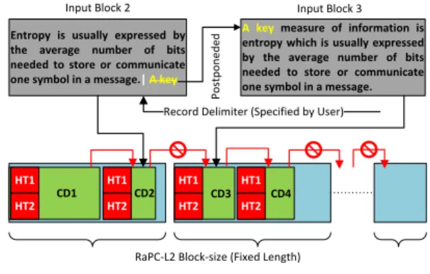
Entropy is usually expressed by the average number of bits needed to store or communicate one symbol in a message.|A key
Input Block 2
A key measure of information is entropy which is usually expressed by the average number of bits needed to store or communicate one symbol in a message.
Input Block 3 P o stp on ed ed
Record Delimiter (Specified by User)
Fig. 3. RaPC Layer-2 record-aware compression.
determining record completeness between L2-Blocks (Fig-ure 2). Recall that Hadoop HDFS organizes big files by split-ting them into a series of fixed-size blocks (HDFS-Block). A series of HDFS-Blocks are distributed across the Hadoop
clusterData Nodes. There is no guarantee that logically
ad-jacent HDFS-Blocks will be stored consecutively and/or on the same physical hard disk. Both the L2-Blocks (referring to
Figure 2CD4andCD5) belong to separate HDFS-Blocks and
are possibly on different physicalData Nodes. The L2-Block
(containingCD5) needs to be streamed to the current Map
node (which is processing the L2-Block containingCD4) and
decompressed. Then, record completeness must be checked. Both scenarios are time consuming and error-prone.
To remove this complication and improve the MapRe-duce work-flow efficiency, we ensure record completeness at the boundaries of each L2-Block during the data compres-sion phase, hence making it record-aware. What constitutes a record is often dataset specific. To determine records, record delimiters must be given at the beginning of the data compression. At the last DI-Block (corresponding to the last DO-Block) of each L2-Block, we check for record completeness. Any partial record will be postponed to the next DI-Block which will eventually be packed into the next L2-Block. This process only occurs between DO-Blocks. An example is shown in Figure 3. Complex delimiters can be
expressed inRegular Expressions. The compression scheme
guarantees that each L2-Block contains a set of complete logical records.
As we have noted, DO-Blocks have variable length and L2-Blocks have fixed size. When packaging a number of consecutive DO-blocks in a L2-Block, there is no guarantee that the L2-Block will be filled up exactly. We need to define a packaging format to tell RaPC how much of the payload is contained in the Block. The gaps at the end of each Block are filled by trailing bytes. The last two bytes of the L2-Block are reserved and used to indicate how many trailing bytes are used. In addition, the MSB of the second last byte is used to indicate whether there is a giant record that spans multiple L2-Blocks. This is designed for an occasion when a dataset contains very long records. Overall, the trailing byte
indicator can only allow215 =32KB of trailing bytes to be
inserted. In the case where there are only a small number of DO-Blocks left for packaging at the end of the compression, the number of trailing bytes needed may exceed this limit.
13.3 13.4 13.5 13.6 13.7 13.8 13.9 14.0 14.1 14.2 14.3 256KB 512KB 768KB 1MB 2MB 3MB 4MB 5MB 6MB 7MB 8MB 9MB 10MB 20MB 30MB
RaPC Block Size
Compressed Size (GB)
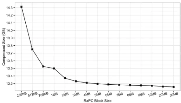
Fig. 4. RaPC Layer-2 block size verses compression ratios
For this reason, an exception is made so that the size of the last L2-Block is the total length of the last several DO-Blocks exactly. That is, no trailing bytes are inserted into the very last L2-Block.
Note that an increase in L2-Block size will slightly im-prove the compression ratio. Figure 4 shows the results from
compressing the datasetDS-WikiEN(the original dataset is
47GB, referring to Table 4) with various L2-Block sizes. In this experiment, we start with a L2-Block size of 256KB and gradually increase the block size to 30MB. In Figure 4, we observe a rapid drop in compressed data size (increased compression ratio) from 256KB to 2MB, and show decrease in compressed data size when the L2-Block size is beyond
2MB. This is due to two reasons.
Firstly, we break the Inter-DO-Block linkages to make the compressed data splittable. This implies that the current DI-Block cannot use the information from its immediate
predecessor for the contents of the currentSliding Window.
The disconnection leads to the compression for the current DI-Block to accumulate its own new context, and at the beginning of this context accumulation phase, much less information can be compressed. This results in a lower compression ratio.
In addition, the Sliding Window is 32KB by default, so
that in the worst case scenario, if no information can be compressed during the context accumulation phase, there will be 32KB of incompressible data at the beginning of every L2-Block. When the L2-Block size is small, the 32KB incompressible data will occupy a relatively large
propor-tion of the total (L2−Block size32KB ) and thus have a bigger
influence on the compression ratio. This is the main cause of the rapid drop in the compressed data size (increase in compression ratio) as the L2-Block size increases.
Secondly, during the L2-Block packaging processes, trail-ing bytes and indicator bytes must be appended to the last DO-Block to fulfil the requirements for a record-aware L2-Block. By increasing the L2-Block size, we have statistically reduced the number of trailing bytes and indicator bytes needed, thus improving compression ratio.
This experiment gives us a general idea how the L2-Block size affects the compression ratio. The results in Figure 4 may vary slightly depending on the contents of a given dataset. Choosing a bigger L2-Block size can improve compression ratio, but it has side-effects on MapReduce pro-gram performance. This will be studied further in Section 5.
4
R
APC
ONH
ADOOPIn order to use RaPC compressed data on Hadoop with maximum transparency to MapReduce programs and de-velopers, we provide a set of utility functions including:
a customized RaPC Record Reader for decoding the
RaPC-L2 compressed data; a RaPC TextWritable data type which
implements equivalent operations found in the HadoopText
data type for handling the RaPC-L1 compressed data; and a
SequenceFileAsBinaryOutputFormat Record Writerfor writing
RaPC-L1 compressed data and general binary data to the HDFS.
The RaPC work-flow is as follows. The RaPC com-pressed files must be stored in the HDFS, and if it is needed, the RaPC-L1 compression model file must be loaded to the
HDFS Distributed Cache. A MapReduce program must set
the provided record reader (RaPCInputFormat) as the default input format class. This ensures that the RaPC Layer-2 com-pressed data can be correctly read and decoded. The input
valuetype for Mappers must be set toRaPCTextWritable or
the regular Texttype. If the data is compressed by
RaPC-L2(L1) (RaPC-L1 embedded in RaPC-L2), then the records received by the Mapper are in fact a block of binary data
in the RaPC Layer-1 compressed format, and the
RaPCTex-tWritabledata type must be used. If the data is compressed
by RaPC Layer-2 only, the decoded data is the original text,
and then the regular Text data type (in the context of the
MapReduce framework) can be used.
For many data analysis jobs, parsing data records is necessary. For the original text, manipulating data is simple as the data contents are readable by developers. In RaPC,
we provide a transformation function T( ) that converts
between original text and RaPC-L1 compressed data. For example, if we write a regular Java clause for searching
a phrase ”value.contains(”big data”);”, then in RaPC it is
simply”value.contains(RaPC.T(”big data”));”. In this example,
the variable ”value” in the regular program can be a String data type. In RaPC, the variable ”value” needs to be declared
as a RaPCTextWritabledata type. The ”contains( )” function
in RaPC is an implementation of the ”contains( )” function
found in the regular Java String class for the
RaPCTex-tWritabledata type. Indeed, the transformation requires the
RaPC-L1 compression model file to be loaded at the Map and/or Reduce initialization phase. This may incur a small
delay due to loading the model files from HDFSDistributed
Cache to the local computational nodes. For some types of
job, for example,N-Gramsanalysis, there is no need to load
model files, and those MapReduce programs can take full advantage of using RaPC.
Another point worth mentioning is that the final MapRe-duce output can be in the original text format or RaPC-L1 compressed format. In the former case, the RaPC-RaPC-L1 decompression needs to be carried out at each Reducer before writing any results to HDFS. The second case needs more attention. By default, writing binary records to HDFS
requires theSequenceFileAsBinaryOutputFormatprovided by
the MapReduce framework. This defaultRecord Writeralso
writes some auxiliary information about each binary record
including recordkey/valuelength and it periodically inserts
synchronization points (0xFF). The recordkey/valuelength
byte sequences; this makes the final output specific to Hadoop. Furthermore, the synchronization point is a char-acter drawn from the extended ASCII codes which is very likely to clash with RaPC-L1 codes and confuse the RaPC-L1 decompression process. An additional requirement for writ-ing the RaPC-L1 compressed output to HDFS is therefore to
use our customizedRaPCSequenceFileAsBinaryOutputFormat
which has synchronization points removed and has well
formattedkey/valuelength.
In general, for a RaPC-L2-enabled MapReduce program, configuring file input format is the only major difference; for an RaPC-L2(L1)-enabled program, we need to load the model file, configure the file input format, output format, and corresponding data types.
5
E
VALUATIONWe evaluate the effectiveness of RaPC in an on-site Hadoop cluster. The cluster consists of six nodes. Each node is configured with dual core Intel E8400 (3.0GHz) CPU, 8GB RAM and 1TB SATA3 hard drive. Nodes are connected to a NetGear GS716T Gigabit Ethernet switch. Specifically, the cluster is configured with Hadoop version 2.6.0 and Linux kernel 2.6.32. The HDFS is configured with single replication and 64MB block size. The MapReduce jobs used in the evaluation are summarized in Table 1. We use several real-world datasets as listed in Table 4 for the evalua-tion. The evaluations of the RaPC compressor and RaPC with MapReduce include measuring analysis performance, cluster storage requirements, memory constraints and com-pression performance. In the experiments, the number of Mappers and Reducers are optimized for each job. RaPC-L2 block-size was set to 1MB across all the experiments. We compare RaPC with the state-of-the-art Hadoop-LZO (also know as LZO-splittable), version 0.4.20.
5.1 Performance
Table 1 contains our main evaluation results. We use ten different MapReduce jobs to evaluate the effectiveness of RaPC on Hadoop with a range of real-world datasets having different properties. We run each job three times with origi-nal, RaPC-L2, and RaPC-L2(L1) compressed data. We record the input data size, intermediate output (Map output) size, final output (Reduce output) size, memory allocation, and analysis duration for each job with the three different input data types.
The Site Rank job is selected to demonstrate the full
advantages of using RaPC with MapReduce. In this job, we calculate the rank for each website in the given dataset based on a ranking algorithm defined for an undirected
graph. According to [39], given an undirected graphG(V, E),
calculating the rank for vertexviinGis equivalent to
calcu-lating the degree distribution ofvi defined by d(v2|Ei|), where
d(vi)is the degree of vertexviinG. Thus the site rank job is
to obtain a vector as given by2|1E|·[d(v0, d(v1),· · · , d(vn)],
where the edgesEare the connections between websitesV.
In fact, the calculation part of the Site Rank job is
rel-atively lightweight. The heavy part is parsing the dataset and finding out all of the connections between websites. The MapReduce job involves parsing the URLs for each website,
then finding and formatting edges E. Using the
RaPC-L2 compressed data for the Site Rank job, we accelerated
the calculation speed by 59.8% compared to that same job with the original text data. The performance gains come from two sources. Firstly, the RaPC-L2 compressed data is approximately four times smaller than the original data (RaPC-L2 reduces the original data size by 74.3%). Loading the RaPC-L2 compressed data from hard disks to memory requires much less time. Secondly, due to the MapReduce
Local Combinereffects, the intermediate data is smaller. This
reduces the time required to transmit data from Mappers to the Reducers over the network.
Additional to the job with RaPC-L2 compressed data, using RaPC-L2(L1) compressed data can further improve the analysis performance. When parsing the URLs, we need to split each URL using the forward slash character ”/”. The results of splitting gives an array of sub-strings drawn from the Web link. We are interested in the website link part only. The access protocol and the page identifier parts must be omitted. The string splitting process is about searching for the delimiter ”/” and taking the sub-string from the link iteratively. By default, the Java implementation of the
stringsplitfunction invokes theindexOf( )function to locate
patterns which takes O(m(n−m))time, where m and n
are the pattern length and source string length, respectively.
In this case, m = 1, therefore each search on pattern ”/”
takesO(n−1)time. Recall that the RaPC-L1 compression
does not compress functional contents. We can search for the forward slash character from the RaPC-L1 compressed data directly without using the model files. The compression ratio for this particular dataset can be found in Figure 6. It is approximately 49%. Theoretically, this implies searching
the same pattern from the new sourceO(n0−1)is
approxi-mately twice as fast asO(n−1), wheren0= 0.49n.
In the second job, we use aN-gramtask for evaluating the
RaPC under intensive disk I/O operations.N-gramanalysis
is a common technique for speech recognition. We use 5-Gram to produce sufficient in-memory data to increase the frequency of memory to disk I/O operations. The job
con-sists of Map tasks only. There are noShufflingandReducing
phases, thus the network I/O is kept to a minimum. Com-paring the results of the original and RaPC-L2 compressed data, RaPC-L2 improves the processing speed by 33.4%. Be-cause both analyses generate the same size output, therefore the main performance gain is from distributing MapReduce data-splits to Mappers. Using RaPC-L2(L1) compressed data
can further improve the analysis speed by∼2.2% because of
the smaller input and output data in RaPC-L1 compressed format.
Besides the efficiency, there is a useful side-effect when
using RaPC-L2(L1) compressed data. Recall that the5-Gram
job reads, manipulates, and writes data in the RaPC-L1 compressed format. During the lifetime of the job, the RaPC-L1 model files are not required. As the RaPC-RaPC-L1
compres-sionencrypts(encodes) the informational contents, using the
RaPC-L2(L1) compressed data can provide a certain level of protection on data privacy in a shared cluster or in a public cloud environment.
TheWord Countjob is used as a standard benchmark for
results comparison. Also, theWord Countjob generates
TABLE 1
A summary of MapReduce jobs used for evaluating RaPC on Hadoop.
Job Dataset Input
Type Input Intermediate Output
Memory Allocation Duration Performance Gain Size Reduction (Input) Site Rank DS-Memes O : 52.5 GB 2.1 GB 20.7 MB 7.5 GB 16m32s H-LZO : 21.0 GB 2.0 GB 20.7 MB 4.1 GB 8m56s 46.0% 60.0% L2 : 13.5 GB 2.0 GB 20.7 MB 3.1 GB 6m39s 59.8% 74.3% L2(L1) : 10.9 GB 1.3 GB 13.8 MB 2.2 GB 4m38s 72.0% 79.2% 5-Gram DS-WikiEN O : 47.0 GB – 150.9 GB 12.7 GB 25m19s H-LZO : 20.5 GB – 150.9 GB 10.0 GB 19m19s 23.7% 65.1% L2 : 13.4 GB – 150.9 GB 8.8 GB 16m52s 33.4% 71.5% L2(L1) : 10.9 GB – 87.6 GB 7.1 GB 16m18s 35.6% 76.8% Word Count DS-StackEX O : 40.6 GB 30.6 GB 9.0 GB 24.1 GB 74m39s H-LZO : 17.3 GB 19.5 GB 9.0 GB 15.8 GB 30m35s 59.0% 57.4% L2 : 11.5 GB 19.1 GB 9.0 GB 14.7 GB 28m33s 61.8% 71.7% L2(L1) : 9.6 GB 16.4 GB 6.3 GB 13.7 GB 26m22s 64.7% 76.4% Publication Indexing DS-PubMed O : 3.1 GB 2.3 GB 482.8 MB 873.2 MB 2m01s H-LZO : 2.1 GB 2.2 GB 482.8 MB 777.4 MB 1m47s 11.6% 32.3% L2 : 1.3 GB 2.2 GB 482.8 MB 736.4 MB 1m38s 19.0% 58.1% L2(L1) : 1.0 GB 1.0 GB 198.6 MB 368.2 MB 1m09s 21.3% 67.7%
Music Rank DS-Yahoo
O : 10.2 GB 235.6 MB 3.2 MB 3.4 GB 6m48s H-LZO : 4.2 GB 294.6 MB 3.2 MB 2.9 GB 5m39s 16.9% 58.8% L2 : 2.4 GB 166.1 MB 3.2 MB 2.3 GB 4m35s 32.6% 76.5% L2(L1) : 2.2 GB 156.6 MB 2.8 MB 2.4 GB 4m37s 32.1% 78.4% L2(L1-C) : 2.2 GB 156.6 MB 3.2 MB 2.5 GB 4m45s 30.1% 78.4% Customer Satisfaction DS-Amazon O : 33.4 GB 223.1 MB 496.2 MB 4.8 GB 10m16s H-LZO : 17.1 GB 194.2 MB 496.2 MB 3.2 GB 6m50s 33.4% 48.8% L2 : 11.1 GB 183.3 MB 496.2 MB 2.0 GB 4m24s 57.2% 66.8% L2(L1) : 8.3 GB 154.8 MB 350.7 MB 3.5 GB 6m48s 33.8% 75.1% L2(L1-C) : 8.3 GB 154.8 MB 496.2 MB 3.5 GB 6m54s 32.8% 75.1% Data Preprocessing DS-Memes O : 52.5 GB 15.1 GB 29.5 GB 7.9 GB 17m56s H-LZO : 21.0 GB 15.0 GB 29.5 GB 4.8 GB 11m33s 35.6% 60.0% L2 : 13.5 GB 15.0 GB 29.5 GB 3.7 GB 8m46s 51.1% 74.3% L2(L1) : 10.9 GB 11.0 GB 16.3 GB 2.3 GB 5m57s 66.8% 79.2% Format Conversion DS-Twitter O : 17.3 GB – 30.4 GB 3.2 GB 6m34s H-LZO : 10.0 GB – 30.4 GB 2.5 GB 5m01s 23.6% 42.2% L2 : 6.5 GB – 30.4 GB 2.0 GB 3m58s 39.6% 62.4% L2(L1) : 6.1 GB – 28.1 GB 1.6 GB 3m18s 49.7% 64.7% Event Identification DS-Google O : 158.9 GB 282.1 MB 32.7 KB 18.1 GB 39m52s H-LZO : 60.9 GB 108.7 MB 32.7 KB 9.5 GB 19m55s 50.0% 61.7% L2 : 36.0 GB 64.8 MB 32.7 KB 6.4 GB 13m12s 66.9% 77.3% L2(L1) : 31.1 GB 56.6 MB 20.9 KB 8.4 GB 16m41s 58.2% 80.4% L2(L1-C) : 31.1 GB 56.6 MB 32.7 KB 8.4 GB 16m49s 57.8% 80.4% Server Log Analysis DS-Google O : 158.9 GB 1.0 GB 371.1 KB 26.3 GB 54m57s H-LZO : 60.9 GB 414.1 MB 371.1 KB 14.6 GB 29m08s 47.0% 61.7% L2 : 36.0 GB 246.8 MB 371.1 KB 11.4 GB 22m26s 59.2% 77.3% L2(L1) : 31.1 GB 196.2 MB 273.5 KB 12.1 GB 23m16s 57.7% 80.4% L2(L1-C) : 31.1 GB 196.3 MB 371.1 KB 12.5 GB 24m04s 56.2% 80.4%
O: Original dataset; H-LZO: Hadoop-LZO; L1: RaPC Layer-1 compression; L2: RaPC Layer-2 compression. The final output is in original format; L2(L1): RaPC Layer-1 embedded in RaPC Layer-2 compression. The final output is in RaPC Layer-1 compressed format; L2(L1-C):
RaPC Layer-1 embedded in RaPC Layer-2 compression. The final output is in original format.1GB = 1,073,741,824 Bytes
RaPC-L2 or RaPC-L2(L1) compressed data, we can reduce the size of the intermediate output by 33.5% and 43.5%, respectively. Thus, the transport cost of distributing the Map output to corresponding Reducers over the network
(MapReduceShuffling phase) can be reduced significantly.
It also reduces the cost of materializing in-memory data to
local persistent storage (local hard disks). The reduction of the size of the intermediate output is due to the MapReduce
Local Combinereffects.
Recall the work-flows in the Map phase, and note that the following parameters are the default values in Hadoop version 2.5.0 or above. When processing a data split, the
Map outputs are temporarily stored in an in-memory buffer (100MB). When the buffer fills to a certain threshold (80%), a background process starts materializing the in-memory data
to the local persistent storage. During thisspillingphase, the
buffered data is firstly partitioned according to the number of Reducers configured for this particular job. Within each
partition, records are sorted bykeys. The sorting results are
then fetched to the Local Combinerprocess to combine the
records with duplicatekeys. The output of theLocal Combiner
is called a ”Spill” and it is then written to local hard disks.
Generally, the data processed by aLocal Combiner is much
smaller depending on the number of records with duplicate
keys found. Thus, we can reduce the time used to writeSpill
data to disks.
For each individual Mapper, if the generated interme-diate data is larger than the in-memory buffer size, each
Mapper will produce a series ofSpills. Upon the completion
of processing a data split, all partitions from the group of
Spillsthat belong to the same Mapper will be merged based
on their partition number and then sorted by record keys.
The sorting results are again fetched to theLocal Combinerto
further examine records with duplicatekeys. This is the place
where the RaPC can reduce the intermediate data size. The reasons are as follows. In any given cluster environment, the HDFS-Block size is fixed. Assume processing each data
split will generatemrecords on average. With the original
text data, theLocal Combinerprocess is about finding records
with duplicatekeysinm. With RaPC compressed data, each
Mapper will receive a block of data with the same size,
but in compressed format. Given the compression ratio ϕ,
defined as ϕ = So−Sc
So , where So denotes the size of the
source file, and Sc denotes the size of the compressed file.
Each Mapper will actually receive Sc
1−ϕ size data. For
in-stance, in thisWord Countjob, assuming that the number of
Map output records are proportional to the Map input data size, using the original text data, each Mapper will receive 64MB (equal to the HDFS-Block size) data split on average
and producemrecords. For the RaPC-L2 compressed data
with a compression ratio of 71.7%, each Mapper will receive 64M B
(1−0.717) ≈ 226MB data (after RaPC-L2 decompression)
and produce∼3.5mnumber of records. Whenmincreases,
we will have a statistically greater chance of finding more records with duplicate keys and/or more duplicate keys for a record, thus further reducing the size of the intermediate outputs. In general the bigger the size of L2-Block, the
more the effects of Local Combiner with RaPC are further
enhanced.
In thePublication Indexingjob, we calculate the
descrip-tive statistics for each publication based on the importance of the author(s) which is further defined by the number of publications from the author. Thereafter, the index of the publication can be sorted by designated statistics. We use
thePubMed database records [40] for this job. The dataset
contains∼22 million publications and∼11 million authors.
Referring to Table 1, RaPC-L2 compresses the data by 58.1% which is the lowest ratio among the ten jobs. Considering the similar intermediate and final output data size, this low compression ratio leads directly to the low performance gain of 19%. Further improvement of 2.3% is given by using the RaPC-L2(L1) compressed data which is the combined contribution from the smaller intermediate and final output
data size.
TABLE 2
Comparison of Map input records for the original, RaPC-L2 compressed and RaPC-L2(L1) compressed data.
Number of Map Input Records
Job Original RaPC-L2 RaPC-L2(L1)
Site Rank 919061195 13810 11160 5-Gram 805750261 13823 11027 Word Count 6126845962 11745 9881 Publication Indexing 21788173 1370 1020 Music Rank 699640226 2435 2268 Customer Satisfaction 381554470 11397 8490 Data Preprocessing 919061195 13810 11160 Format Conversion 468854886 6622 6232 Event Identification 1232799308 36915 31840
Server Log Analysis 1232799308 36915 31840
In the Music Rank job, we use the Yahoo! Music Rating
dataset [41] which contains a large number of very small records (approximately 16 characters per record on average).
The dataset contains∼700 million ratings on∼136 thousand
songs provided by Yahoo! Music services. The task is to
calculate the mean scores and standard deviation for each
song. For this task, the MapReduceRecord Readersare
heav-ily loaded supplying records to the corresponding Mappers.
The default Record Reader provided by the MapReduce
framework treats a line as a record. The records processed by a Mapper will have on average 16 characters. This makes
the defaultRecord Readerinefficient and wastes a lot of
clus-ter resources such as Java Heap Space (memory) assigned
to the Mapper. With compressed contents, our
RaPCRecor-dReaderis in fact supplying a set of records to a Mapper at
a time. Table 2 shows the number of records received by Mappers for each job with different input data. It works by reading a fixed-size block of data (Block, the size of L2-Block is adjustable). The block of data will be decompressed in-memory and then forwarded to a Mapper. Because the L2-Block size is fixed, and more importantly, each L2-Block contains a set of complete records, there is no need to track record length and worry about partial records at the boundaries of L2-Blocks and HDFS-Blocks. This makes the
RaPCRecordReader more efficient and lightweight than the
default MapReduceRecord Reader. Additional to the
RaPC-L2(L1) compressed data, in order to calculate music scores,
we must convert the text contents to real numerical values. This conversion requires loading the RaPC-L1 compression model files to each Mapper. The loading process and the text to numerical value conversion take extra time and occupy more memory. This leads to the job with the RaPC-L2(L1) compressed data being slightly slower than the job with RaPC-L2 compressed data.
The Customer Satisfaction job is a special case. When
processing RaPC-L2 compressed data, the job results in a relatively high performance gain of 57.2%. Two sources contribute most to this result. The first source is the lower data transmission cost due to the smaller data size. The
second source is the Group Record Effect. Records in this
particular dataset are split by empty line(s). Each record consists of multiple fields delimited by a new line character.
Records contain a variable number of fields. By default, the MapReduce framework treats the new line character as the
delimiter. The default Record Readersupplies a line of text
to a Mapper at a time. This requires Mappers to wait for
theRecord Readeruntil a full logical record is received. The
waiting time is the main cause of the delay. With RaPC compressed data, a group of complete records are given to one Mapper at a time, and therefore, it saves on waiting
time. Indeed, writing a customized Record Reader using a
traditional approach for this particular dataset can improve the analysis performance on the original dataset. But, it will incur extra programming and will still suffer from the big data size.
TheData Preprocessing job is used to evaluate the
effec-tiveness of RaPC-L2(L1) when dealing with highly skewed giant records. In this job, we create records that have a
source website link as thekeyand all web pages that refer
to the source website as the value. The preprocessed data
thereafter can be used for other calculations, for example, web site popularity and centrality analysis. We can use the
Memetracker memesdataset [42]. It contains∼418 million web
page URLs. Some extremely popular websites are referenced by many web pages. Formatting and appending the refer-ring web page links to a source website can result in a giant record. If the size of the giant record is larger than the size of the Java Heap Space that is currently available to the Mapper, it will cause very frequent in-memory data to disk swapping processes. The disk I/O bursts were observed in both the tasks with original text and RaPC-L2 compressed text. This irregular event also causes extra delay to the job completion time.
In contrast, when processing RaPC-L2(L1) compressed data, it is hard to identify any obvious disk I/O bursts. Referring to Figure 6, the RaPC-L1 compression ratio for
this particular dataset is∼49%. Generally, the Map output
records are half the length of those produced by the same tasks with either original or RaPC-L2 compressed text. Additionally, in the previous version of Hadoop, when the record size is larger than the size of the Java Heap Space available to the Mapper, the MapReduce framework will
throwJava Heap Space Errors, and the corresponding
parame-ter ”mapred.reduce.child.java.opts” needs to be re-adjusted to a bigger value and then the entire cluster needs to be restarted
to pick up the changes. TheFormat Conversionjob is similar
to the previous task.
The Server Log Analysisand the Event Identification jobs
are used to evaluate RaPC with comparatively large jobs.
The main task of the Server Log Analysis is to determine
the over/under utilized servers from Google Cluster Log
files [43]. The dataset contains ∼1.2 billion records in
Comma Separated Value (CSV) format. For this particular dataset, RaPC-L2 and RaPC-L2(L1) can reduce the original data size by 77.3% and 80.4%, respectively. The size of the intermediate output is significantly smaller because of the
MapReduceLocal Combinereffects discussed above and the
highly repetitive nature of the data. Due to the significant data size reduction (both input and intermediate output), we have achieved 59.2% and 57.7% performance gains from the job with RaPC-L2 and RaPC-L2(L1) compressed data, respectively. During the analysis, numerical values in the RaPC-L1 format need to be decoded to standard strings
SiteRank 5-Gram WordCount PublicationIndexing MusicRank
CustomerSatisfaction DataPreprocessing FormatConversion EventIdentification ServerLogAnalysis
0 200 400 600 800 0 200 400 600 0 200 400 600 0 10 20 30 40 50 0 50 100 150 0 200 400 0 200 400 600 800 0 100 200 0 1000 2000 0 1000 2000 Dataset
Number of Map Processes
Hadoop-LZO Original RaPC-L2 RaPC-L2(L1)
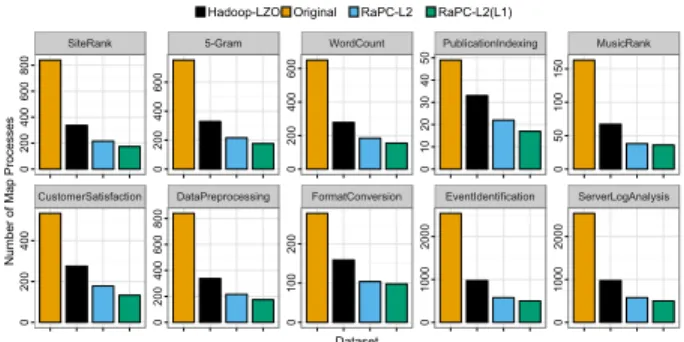
Fig. 5. Number of Map processes for each job (default to Hadoop) with original, RaPC-L2 compressed and RaPC-L2(L1) compressed data.
and then converted into real numerical values. This requires the RaPC-L1 compression model file to be available for each Mapper, which makes RaPC-L2(L1) job slower than the job with the RaPC-L2 compressed data. The level of the performance degradation is influenced by the number of Mappers and how much RaPC-L1 compressed data needs to be decoded during the analysis. If we increase the HDFS-Block size (equivalent to reduce the number of Mappers), we can improve analysis speed and memory consumption, accordingly. Note that the RaPC-L1 compression model file needs to be loaded to each Mapper separately. The smaller number of Mappers results in less memory (aggregated) being used to hold the RaPC-L1 models. Rationally, if a considerable portion of the RaPC-L1 data needs to be de-coded during the job execution, then just using the RaPC-L2 compression for the data is a more appropriate approach.
This also applies to theEvent Identificationjob.
In general, using the RaPC-L2 or RaPC-L2(L1) com-pressed data requires much less memory. The reasons are as follows. Firstly, Mappers are independent processes and require dedicated Java Virtual Machines (JVMs). Each has a default and dedicated Java Heap Space assigned to it. The more Mappers the more memory is required. Because the input data size is the dominant factor affecting the number of Mappers, the compressed data size is significantly smaller resulting in a smaller number of Mappers and consequently less aggregate memory consumption. Figure 5 shows the default number of Mappers configured for each job with the original, RaPC-L2, and RaPC-L2(L1) compressed data. Moreover, supplying a block of data to a Mapper at a time can make more efficient use of the memory .
Furthermore, we compare the RaPC scheme with the
state-of-the-artHadoop-LZO. UsingHadoop-LZOcompressed
data in Hadoop is similar to our RaPC scheme.
Hadoop-LZO compresses data using the standard LZO
compres-sor. The compressed data is then uploaded to HDFS. A special indexer program is used to index and record the splittable boundaries of the compressed data. The output of the indexer is a set of indexing files which are associated with each individual dataset. In MapReduce, each Mapper uses the indexing files to calculate splittable boundaries and take the data block for processing. As the number of datasets increases, maintaining and processing the indexing files can be complicated. The main comparison results are shown in Table 1. In general, using RaPC compressed data
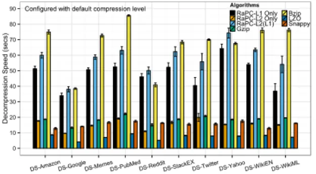
Configured with default compression level 0 10 20 30 40 50 60 70 80 90 100 DS-AmazonDS-GoogleDS-MemesDS-PubMedDS-RedditDS-StackEXDS-TwitterDS-YahooDS-WikiENDS-WikiML Compression Ratio (%) Algorithms RaPC-L1 Only RaPC-L2 Only RaPC-L2(L1) Gzip Bzip LZO Snappy
Fig. 6. RaPC compression ratio comparing toBzip,GzipandLZOwith
default compression level .
can improve MapReduce performance by 13.5% (RaPC-L2) and 15.1% (RaPC-L2(L1)), and can further reduce data size by 16.2% (RaPC-L2) and 21.0% (RaPC-L2(L1)), on average,
compared to that usingHadoop-LZOcompressed data.
In brief, we have demonstrated the flexibility and effec-tiveness of using RaPC with MapReduce using a variety of standard MapReduce jobs. Using RaPC-L2 does not exhibit any shortcomings and RaPC-L2(L1) can further improve efficiency of analysis speed, cluster memory usage, and storage usage. It can be most beneficial to clusters that are I/O bound and for whom storage space is a concern. For some jobs that need many conversions, for example,
financial report analysis, using theT( )function frequently
can affect the overall performance. In those cases, using RaPC-L2 compression alone may be more appropriate.
5.2 RaPC Characteristics
In this section, we evaluate the characteristics of RaPCL1, -L2, and -L2(L1) schemes in terms of compression ratio, com-pression speed and decomcom-pression speed. The results are thereafter compared with four common compressors that are currently supported by the Hadoop system, including
Gzip (v1.6), Bzip (v1.0.6), LZO (v1.03) and Snappy (v1.1.2).
Exactly 2GB of data is drawn from each dataset (as shown in Table 4) for the experiments. There are five runs for each
experiment. The compression ratio forGzip,Bzip,LZOand
Snappy are identical across the five runs. In contrast, there are some slight variations in the RaPC-L1, -L2, and -L2(L1) compression results due to the random sampling effects. The compression and decompression speed also varies slightly due to system variation of the testbed. The mean values and standard mean errors are calculated and included in the ex-perimental results. All experiments are carried out on Linux kernel version 3.19.0 and x86 64 architecture platform with dual WD5000AAKS-75V0A0 500GB hard disks (7200RPMs)
andExt4(version 1.0) file system.
5.2.1 Compression Ratio
Compression ratio is content dependent. Figure 6 shows the
compression results for RaPC,Gzip,Bzip,LZOandSnappy.
Specifically, Gzip, Bzip and LZO are configured with the
default compression level settings. RaPC-L1 can compress
data by∼50% on average. There are two exceptions: dataset
DS-Twitter and dataset DS-WikiML. Recall that RaPC-L1
does not compress Unicode contents. DatasetDS-WikiMLis
multi-language Wikipedia articles, where the majority of the contents are complex Unicode texts which are
incompress-ible. Additionally, we must use the0x11and0x12character
pair to enclose any Unicode strings. This leads to the low
RaPC-L1 compression ratio on datasetDS-WikiML. Dataset
DS-Twitter contains ∼490 million Twitter tweets collected
world wide. A large number of records contain Unicode texts. Moreover, each tweet record is comprised of a time-stamp, anonymized user ID which is often a hash code, and tweet topics. This makes the vocabulary size for the dataset much larger. Considering that the RaPC-L1 code length increases with the vocabulary size, this makes the average code-length longer for the dataset. In practice, if the the data is known to contain many Unicode strings, it is better to avoid using RaPC-L1 compression at all.
RaPC-L2 is a block-based compression based on the
De-flatealgorithm. In principle, RaPC-L2 can achieve the same
compression ratio asGzip. Recall that, in RaPC-L2
compres-sion, we intentionally break the connections between DO-Blocks and stuff trailing bytes at the end of each L2-Block;
this makes RaPC-L2 compression slightly worse thanGzip.
In fact, RaPC-L2 compression ratio is very close toGzip.
RaPC-L2(L1) is a composite compressor. It applies the RaPC-L2 compression on the RaPC-L1 compressed data.
In practice, it can achieve compression ratios close to Bzip
and sometimes even better than Bzip. For example, the
compression results fromBzipand RaPC-L2(L1) for dataset
{DS-Google, DS-Memes, DS-Twitter, DS-WikiEN} are given
by{{152.2MB, 150.5MB},{465.6MB, 442.4MB}, {663.5MB,
663.3MB},{456.3MB, 427.1MB}}, respectively.
5.2.2 Compression Speed
Configured with default compression level
0 50 100 150 200 250 300 350 400 DS-AmazonDS-GoogleDS-MemesDS-PubMedDS-RedditDS-StackEXDS-TwitterDS-YahooDS-WikiENDS-WikiML
Compression Speed (secs)
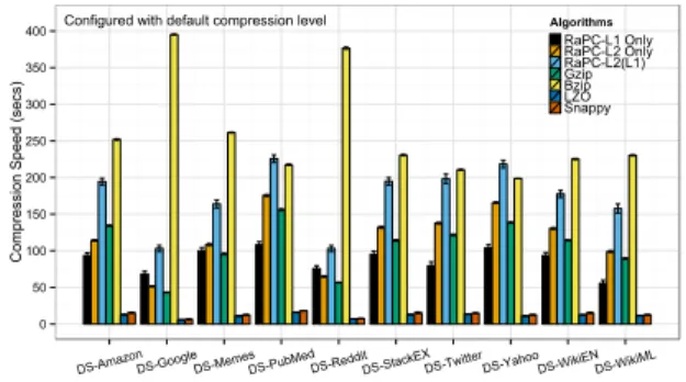
Algorithms RaPC-L1 Only RaPC-L2 Only RaPC-L2(L1) Gzip Bzip LZO Snappy
Fig. 7. RaPC compression speed comparing toBzip,GzipandLZOwith
default compression level .
For compression speed, the current implementation of
RaPC-L2 achieves similar speed toGzip, and RaPC-L2(L1)
is similar to Bzip. Figure 6 shows the compression speed
with default compression levels configured for Gzip, Bzip
andLZO. In general,Bzipis the slowest compressor, because
it has an extra step for block sorting. The speed is often
influenced by block size.LZOis the fastest on
decompres-sion. In contrast, RaPC-L2 and Gzip are relatively stable
and consistent. Figure 6 shows the decompression speed for each compressor configured with default compression levels. Furthermore, we compare the RaPC scheme with the
state-of-the-artHadoop-LZO. UsingHadoop-LZOcompressed
data in Hadoop is similar to our RaPC scheme.