Anomaly detection using network traffic characterization

ANOMALY DETECTION USING NETWORK

TRAFFIC CHARACTERIZATION

A Thesis Submitted to

the Graduate School of Engineering and Sciences of

İzmir Institute of Technology

in Partial Fulfillment of the Requirements for the Degree of

MASTER OF SCIENCE

in Computer Software

by

Oğuz YARIMTEPE

July 2009

İZMİR

We approve the thesis of Oğuz YARIMTEPE

Asst. Prof. Dr. Tuğkan TUĞLULAR Supervisor

Asst. Prof. Dr. Tuğkan TUĞLULAR Committee Member

Asst. Prof. Dr. Tolga AYAV Committee Member

Prof. Dr. Şaban EREN Committee Member

6 July 2009

Prof. Dr. Sıtkı AYTAÇ Prof. Dr. Hasan BÖKE

Head of the Computer Engineering Department

Dean of the Graduate School of Engineering and Sciences

ABSTRACT

ANOMALY DETECTION USING NETWORK TRAFFIC

CHARACTERIZATION

Detecting suspicious traffic and anomaly sources are a general tendency about approaching the traffic analyzing. Since the necessity of detecting anomalies, different approaches are developed with their software candidates. Either event based or signature based anomaly detection mechanism can be applied to analyze network traffic. Signature based approaches require the detected signatures of the past anomalies though event based approaches propose a more flexible approach that is defining application level abnormal anomalies is possible. Both approach focus on the implementing and defining abnormal traffic. The problem about anomaly is that there is not a common definition of anomaly for all protocols or malicious attacks. In this thesis it is aimed to define the non-malicious traffic and extract it, so that the rest is marked as suspicious traffic for further traffic. To achieve this approach, a method and its software application to identify IP sessions, based on statistical metrics of the packet flows are presented. An adaptive network flow knowledge-base is derived. The knowledge-base is constructed using calculated flows attributes. A method to define known traffic is displayed by using the derived flow attributes. By using the attributes, analyzed flow is categorized as a known application level protocol. It is also explained a mathematical model to analyze the undefined traffic to display network traffic anomalies. The mathematical model is based on principle component analysis which is applied on the origin-destination pair flows. By using metric based traffic characterization and principle component analysis it is observed that network traffic can be analyzed and some anomalies can be detected.

ÖZET

AĞ TRAFİĞİ KARAKTERİSTİĞİNİ KULLANARAK

ANOMALİ TESPİTİ

Trafik analizindeki en temel yaklaşımlardan birisi de şüpheli trafiğin tespit edilmesidir. Network trafiği ile ilgili anomali tespitine olan ihtiyaçtan dolayı farklı yaklaşımlar ve bunların yazılım çözümleri geliştirilmiştir. Network trafiğinin incelenmesinde olay tabanlı veya imza tabanlı bir yaklaşım sergilenebilir. İmza tabanlı yaklaşımlar önceden yaşanmış anormalliklerden çıkarılan imzalara dayanırken olay tabanlı yaklaşımlar daha esnek bir şekilde anormalliklerin ifade edilebilmesini sağlar. Her iki yaklaşımda da anormal trafiğin ifade edilebilmesi gerekmektedir. Anomali ile ilgili genel sorun ise, her protokol ve durum için genel bir ifade biçimin olmayışıdır. Bu tez çalışmasında, normal trafiğin tanımlanması amaçlanmıştır. Gözlemlenen trafikten normal olarak tanımlanan trafik çıkarılarak kalan trafiğin şüpheli olarak incelenmesi hedeflenmiştir. Bu hedefi gerçeklemek için IP oturumlarına ve istatistiksel metrik değerlerine bağlı ağ paket akışları kullanılmıştır. Ağ akışları ile ilgili gerçeklenebilir ve ağdaki akışların davranış özelliklerini ifade eden bir veri tabanı oluşturulmuştur. Akış özelliklerinden yola çıkarak trafik karakteristiği çıkarma yöntemi açıklanmıştır. Akış özellik değerleri kullanılarak trafik karakteristiğinin nasıl yapıldığı gösterilmiştir. Ayrıca, ele alınan trafik ile ilgili anormallik tespitinde kullanılabilmesi için de matematiksel bir model açıklanmıştır. Birincil Bileşen Analizi (Principle Component Analysis) isimli bu yöntem ile kaynak-hedef çiftlerini içeren akışlar için grafiksel olarak anomali tespit edilebildiği gösterilmiştir. Böylece, incelenen trafiğin karakteristiği çıkarılarak şüpheli trafik üzerinde nasıl anomali tespiti yapılacağı açıklanmıştır.

TABLE OF CONTENT

2.2. Network Flow Tools ...11

2.2.1. Argus...11

2.3. Network Packets...13

2.4. Network Packet Tools...14

2.4.1. Tcpdump...14

2.4.2. Wireshark...15

2.4.3. Tcpreplay...15

2.5. Principle Component Analysis...16

2.5.1. Tools Used Through PCA Process...19

2.5.1.1. Octave...19 2.5.1.2. Snort...20 2.5.1.3. Ettercap...20 2.5.1.4. Nmap...21 CHAPTER 3. APPROACH...22 3.1. Principle of Approach...22

3.2. Processing of Captured Data ...24

3.3. Processing of Flow Data ...27

3.4.1. Discrete Distribution Attributes for Payload and Inter-Packet

Delay...29

3.4.2. Conversations and Transactions...30

3.4.3. Encryption Indicators...32

3.4.4. Command Line and Keystroke Indicators...33

3.4.5. File Transfer Indicators...34

3.5. Deriving Anomaly...35 CHAPTER 4. IMPLEMENTATION...37 4.1. Programming Language...37 4.2. Class Structure ...38 4.2.1. Flow Object...38 4.3. Software Structure ...42

CHAPTER 5. TEST RESULTS...45

5.1. PCA Tests...45

5.1.1. Tests with Clean Traffic...45

5.1.2. Tests with Manual Attacks...47

5.2. Threshold Tests...49

5.3. BitTorrent Traffic Analysis...53

5.3.1. BitTorrent Protocol...53

5.3.2. Testbed for BitTorrent Characterization...54

5.3.3. Criteria for BitTorrent...55

CHAPTER 6. CONCLUSION...61

REFERENCES...63

APPENDICES APPENDIX A...67

LIST OF FIGURES

Figure Page

Figure 2.1. Unidirectional Flow Demonstration, From Source to Destination ...6

Figure 2.2. Unidirectional Flow Demonstration, From Destination to Source ...6

Figure 2.3. Bidirectional Flow Between Two Endpoints ...6

Figure 3.1. Steps Through Anomaly Detection...23

Figure 3.2. Total Bits Per Second for Week 1 Day 1 Record...25

Figure 3.3. Total Number of Packets for Week 1 Day 1 Record... 26

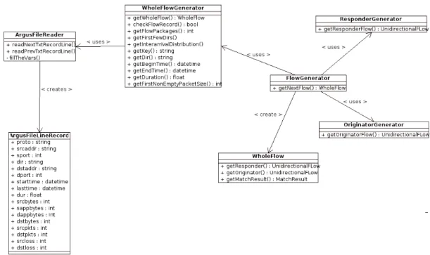
Figure 4.1. AbstractFlow Diagram... 38

Figure 4.2. FlowGenerator and WholeFlowGenerator Class Relations... 39

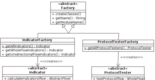
Figure 4.3. Factory Class Diagram... 40

Figure 4.4. Indicator Class Diagram... 40

Figure 4.5. Recognizer Class Diagram... 41

Figure 4.6. Threshold Calculation Sequence Diagram... 41

Figure 4.7. PCA Sequence Diagram... 42

Figure 5.1. PCA Analysis of Week 1 Day 1 Record... 46

Figure 5.2. PCA Analysis of Week 5 Day 2 Record... 46

Figure 5.3. Ettercap DOS Attack PCA Analysis... 48

Figure 5.4. Snort Result of Undefined Traffic, DOS Attack... 48

Figure 5.5. Nmap Syn Scan PCA Analysis... 49

Figure 5.6. FTPCommand Test Results... 49

Figure 5.7. FTPData Test Results... 50

Figure 5.8. HTTP Test Results...50

Figure 5.9. POP Test Results...51

Figure 5.10. SMTP Test Results... 51

Figure 5.11. SSH Test Results... 52

Figure 5.12. Telnet Test Results...52

Figure 5.13. Protocols Similarities Defined for Torrent Traffic...54

Figure 5.14. Payload Distribution Graph for Originator... 55

Figure 5.15. DatabyteRatioOrigToResp Distribution Graph... 56

Figure 5.17. DataByteCount/ByteCount Graph for Originator... 57

Figure 5.18. firstNonEmptyPacketSize of the Whole Flow ... 57

Figure 5.19. P2P Test with FTPData ... 58

Figure 5.20. FTP Data Test with P2P... 59

Figure 5.21. Telnet Test with P2P... 59

LIST OF TABLES

Table Page

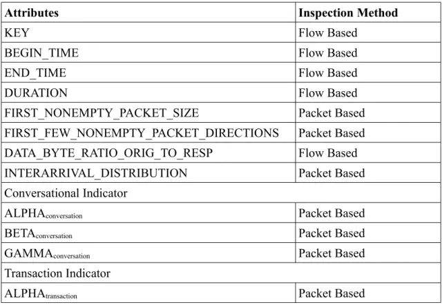
Table2.1. Attributes measured over the whole flow...9

Table 2.2 Attributes measured for each direction of the flow... 10

Table 3.1. Table structure for table FlowPkgTbl... 26

Table 3.2. Conceptual illustration of discrete payload distribution... 30

Table 3.3. Conceptual illustration of discrete packet delay distribution...30

CHAPTER 1

INTRODUCTION

Network traffic measurement provides basic traffic characteristics, supplies information for the control of the network, allows modeling and provides an opportunity to develop and plan the use of network resources. It also enables developers to control the quality of network service operations. Although network traffic measurement is a well-known and applicable area, a general method for detecting anomalies in network traffic is an important, unsolved problem (Denning 1986).

Anomaly detection can be described as an alarm for strange system behavior. The concept stems from a paper fundamental to the field of security, An Intrusion Detection Model, by Denning (Denning 1986). In it, she describes building an "activity profile" of normal usage over an interval of time. Once in place, the profile is compared against real time events. Anything that deviates from the baseline, or the norm, is logged as anomalous. So, anomaly detection systems establish a baseline of normal usage patterns, and anything that widely deviates from it gets flagged as a possible intrusion. A good example for this approach is Bro-IDS (Bro-IDS 2009). It works as en event based intrusion detection system, that is it does not rely on only signatures, recorded and generated by observing previously seen anomalies, but also event definitions that enables dynamic approach to intrusion detection systems. By using its own language, it is possible to define anomalies on application level. Such an event based approach enable further protection for the unseen anomalies. Another anomaly detection system works using signatures that are previously recorded. Since its dependency to previous anomalies and signature collection, signature based systems are not as dynamic as event based systems.

The network traffic to be an anomaly can vary, but normally, any incident that occurs on frequency greater than or less than two standard deviations from the statistical

norm can be approached as a suspicious event. Since the ambiguity on determination of the statistical norm, a general method for detecting anomalies in network traffic doesn't have a unique solution. Basically, it should be possible to observe most anomaly types by inspecting traffic flows. However, to date, there is not a common approach to anomaly detection. There are many good reasons for this: Traffic flows present many possible types of network traffic, the set of all flows occupies a very high-dimensional space, and collecting all traffic flows is very resource-intensive.

In this thesis, detecting anomalies are achieved neither signature nor signature based. Both approaches require definition of an anomaly either in a signature way or an application level protocol way. Instead of defining abnormal traffic, it is presented that, defining normal traffic behavior is easier. By using the normal traffic characteristics, the rest of the traffic can be extracted as suspicious traffic for anomaly detection.

Throughout this thesis, it is shown that traffic flow attributes can be used to define known traffic, which covers application level protocols like FTP, TELNET, SSH, HTTP, HTTPS, IMAP, POP, SMTP, MSN CHAT, RLogin, BitTorrent. Network traffic is taken into consideration as combination of directional flows. For each flow, flow attributes are calculated either using flow metrics or packet based inspection. Packet based inspection includes traversing through the collected packets that belong to a flow session. Especially, attribute values related with statistical analysis requires packet based inspection.

By using the attribute values, it is possible to calculate a match result for each application level protocol. By looking at the match result of the calculated values, it is seen that it is possible to define a threshold value for each protocol and any flow that is under the defined threshold value can be marked as undefined for further inspection. When the undefined flows are observed as a whole and principle component analysis is applied over byte and packet number level, it is seen that the generated graphs has peeks that displays suspicious anomalies over time intervals. For calculating the principle components, number of packets, number of bytes and number of IP flow values are used for each origin-destination pairs. Origin-destination pairs are calculated for the splitted time series of the undefined traffic.

The exact number of applications that contribute to the network traffic is not known and even the actual impact of well-known protocols is not clear. This is due to

the shortcomings of the state-of-the-art in traffic monitoring, which make use of registered and well-known port numbers to classify packets and computer statistics. The problem is new applications often do not use a registered port, do not have a fixed port number, or simply disguise themselves using the port numbers of another application (for example, the web's port 80) to avoid detection (so they can pass through firewalls, and avoid rate limits) (Hernandez-Campos, et. al. 2005).

This thesis will cover mathematical models for traffic characterization, anomaly detection and implementation of them on network traffic. Chapter 2 aims to give a background information. Flow explanations like directionality or flow metrics and tools that are used either on packet or flow based are explained throughout this chapter. This chapter also covers the background information about principle component analysis that is used for anomaly detection for the suspicious traffic. Chapter 3 explains the model of the solution. It is aimed to answer the how part of the thesis. Before starting the implementation phase it is aimed to give logical methodical steps that will be follow to gather anomalies at the network traffic. Chapter 4 covers the implementation details starting from the programming language itself to UML diagrams of the class hierarchy. Chapter 5 includes test results of the particular application level protocols. The results are used to detect threshold for each protocol. Chapter 5 also includes the test results related with the BitTorrent traffic which is added to this thesis as a contribution for the related work. The thesis ends with a conclusion and a further work part.

CHAPTER 2

BACKGROUND

This section aims to provide a background for the concepts used in this thesis. To provide the reader a familiarity with the topics covered through this thesis, this section is divided into three subsections. First section is dedicated for network flow explanations. Flow notion, flow based metrics, directionality and flow attributes are explained in detail. This category also includes the tools used for calculating flow metrics. The second sub section is for packet based inspection and packet based tools used throughout this thesis. In this thesis work, it is also mentioned an anomaly detection method that can be applied on to the flow records, which is called principle component analysis (PCA). Mathematical details about PCA calculation is given at the third subsection of this section.

2.1. Network Flows

2.1.1. Notion of Flow

The notion of flow was introduced within the network research community in order to better understand the nature of Internet traffic. Flow is the sequence of packets or a packet that belonged to certain network session(conversation) between two hosts but delimited by the setting of flow generation or analyzing tool (Lee 2008, June). Network flow data represents a summary of conversation between two end points. It provides valuable information to assist investigation and analysis of network and

security issues. Unlike deep packet inspection, flow data does not rely on packet payloads. Instead the analyst relies on information gathered from packet headers and its associated metrics. This provides the analyst a neutral view of network traffic flow by tracking network sessions between multiple endpoints simultaneously. In addition, having network flow data will provide a better visibility of network events without having the need to perform payload analysis. It is convenient for protocol analysis (Lee 2008, May) or debugging.

In 1995, the IETF’s Realtime Traffic Flow Measurement (RTFM) working group was formed to develop a frame-work for real-time traffic data reduction and measurements (RTFM 1995). A flow in the RTFM model can be loosely defined as the set of packets that have in common values of certain fields found in headers of packets. The fields used to aggregate traffic typically specify addresses at various levels of the protocol stack (e.g. IP addresses, IP protocol, TCP/UDP port numbers). Herein, it is used the term key to refer to the set of address attributes used to aggregate packets into a flow.

2.1.2. Flow Directionality

Flow definition is given above as summary of conversation between two end points. The endpoints here are defined as follows:

a. Layer 2 Endpoint - Source Mac Address | Destination Mac Address Layer 3 Endpoint - Source IP Address | Destination IP Address Layer 4 Endpoint - Source Port | Destination Port

The conversation between these two ends has a direction so flow tool display a direction information related with the flow also. There are two types of direction information related with a network flow. A flow can be defined either as a unidirectional flow or as a bidirectional flow.

At unidirectional flow model, every flow record contains the attribute of single endpoint only. Figure 2.1 and Figure 2.2 show directionality in a more simple way (Lee

2008, June).

At bidirectional flow model every flow record contains the attribute of both endpoints. Figure 2.2 illustrates it (Lee 2008, June):

To make the directionality more clear lets assume that source host sends 90 bytes to destination host and destination host replies with 120 bytes. If the flow communication between these two hosts are unidirectional, then the flow information will be as follows:

Figure 2.1. Unidirectional Flow Demonstration, From Source to Destination

Figure 2.2. Unidirectional Flow Demonstration, From Destination to Source

b. Srcaddr Direction Dstaddr Total Bytes Source Host -> Destination Host 90

Destination Host -> Source Host 120

Though, if the flow communication is bidirectional, then the result will be different:

c. Srcaddr Direction Dstaddr Total Bytes Src Bytes Dst Bytes

Source Host <-> Destination Host 210 90 120

In unidirectional flow, it is only seen the total bytes that sent by source host but nothing about destination in the first flow record. Then the next record shows destination sends 120 bytes to source. The total bytes is accounted from single endpoint only. But in bidirectional flow, it can be seen that source host sends 90 bytes and destination replies with 120 bytes. The total bytes is the accumulation of source and destination bytes.

2.1.3. Flow Identification

Giving a unique label to a flow information depends on the aim of the analysis related with it. If the intent is to analyze the amount of traffic between two hosts, then the focus can be source and destination IP addresses. However, a finer intent like considering the flow information over a state approach to identify connections will require additional information. To identify each flow it is used 5-tuple key representation. The tuple includes source IP address, source port number, destination IP address, destination port number and protocol information.

2.1.4. Flow Period

Flow period means the time periodically report on a flow's activity. The period determines the start and end times of each flow. There are three primary expiry methods

that are appropriate for studying characteristics of individual flows: protocol based, fixed timeout, and adaptive timeout (Keys, et. al. 2001). With protocol based mechanisms, the state of a flow is determined by observing protocol specific messages (e.g. TCP SYN, FIN or RST). With a fixed timeout method, a flow has expired when some fixed period has elapsed since the last packet belonging to that flow was captured. An adaptive timeout strategy is a little more sophisticated than a fixed timeout method. The timeout is different for each flow and is computed based on the packet rate observed so far within each flow.

In this thesis, because of its simplicity a fixed timeout approach is chosen over an adaptive timeout mechanism to decide the expiration time of flows. The timeout value is chosen as 60 seconds for preliminary examination, which is also commonly used in related works (Xu, et.al. 2005) (Claffy, et.al. 1995) (Karagiannis, et.al. 2005).

2.1.5. Flow Attributes

In the literature, flow attributes are often called features, or characteristics. According to the RFTM Architecture (RFC2722 1999) a flow has computed attributes that are derived from end point attribute values, metric values like packet and byte counts, time values as well as summary information like mean, median or average values, jitters and distributional information. The goal in defining flow attributes is to identify now only the relevant characteristics but also the proper way to measure them.

In 2005, De Montigny and Leboeuf published the definition of flow attributes that can be used to characterize a flow at their paper (De Montigny and Leboeuf 2005). At their work it is mentioned nearly thirty property that can be derived from a flow information. The mentioned flow metrics are also used throughout this thesis. The following sub sections will be covering the details of the flow attributes mentioned at the De Montigny and Leboeuf's work (De Montigny and Leboeuf 2005).

Flow attributes are examined in two categories. One of the categories includes the whole flow values, while the second one includes values per directional flows. The attributes derived are summarized in Table 2.1 and Table 2.2. The following sub sections will describe each attribute with greater detail. Table 2.1 lists the attributes that

are measured over the entire flow. The first three attributes (Key, BeginTime, EndTime) are simply used to identify and sort the flows. Table 2.2 gives the attributes that are specific to each direction, and thus are measured in each direction separately. The details of Table 2.1 and Table 2.2 can be found at Appendix A.

Table 2.1. Attributes measured over the whole flow

Attributes Inspection Method

KEY Flow Based

BEGIN_TIME Flow Based

END_TIME Flow Based

DURATION Flow Based

FIRST_NONEMPTY_PACKET_SIZE Packet Based FIRST_FEW_NONEMPTY_PACKET_DIRECTIONS Packet Based DATA_BYTE_RATIO_ORIG_TO_RESP Flow Based INTERARRIVAL_DISTRIBUTION Packet Based Conversational Indicator

ALPHAconversation Packet Based

BETAconversation Packet Based

GAMMAconversation Packet Based

Transaction Indicator

Table 2.2. Attributes measured for each direction of the flow

Attributes Inspection Method

INTERARRIVAL_DISTRIBUTION Packet Based

PAYLOAD_DISTRIBUTION Packet Based

BYTE_COUNT Flow Based

DATA_BYTE_COUNT Flow Based

PACKET_COUNT Flow Based

DATAPACKET_COUNT Flow Based

Encryption Indicators

ALPHAchipherblock Packet Based

BETAchipherblock Packet Based

Keystroke Interactive Indicator

ALPHAkey_interactive Packet Based

BETAkey_interactive Packet Based

GAMMAkey_interactive Packet Based

DELTAkey_interactive Packet Based

EPSILONkey_interactive Packet Based

Command-line Interactive Indicator

ALPHAcmd_interactive Packet Based

BETAcmd_interactive Packet Based

GAMMAcmd_interactive Packet Based

DELTAcmd_interactive Packet Based

EPSILONcmd_interactive Packet Based

File transfer Indicators

ALPHAconstantpacketrate Packet Based

BETAfile Packet Based

GAMMAfile Packet Based

As it can be seen from Table 2.1 and Table 2.2, attributes related with whole flow or each direction of flow have indicators. Indicators generally depend on packet based calculations and enables to derive application level information from flow itself. Although it is mentioned they are calculated mainly by packet based inspection, some of them also use flow based data to calculate some indicator values. Details about the indicators are mentioned at the next section.

2.2. Network Flow Tools

Custom flow tools ease the work on flow data. They reconstructs the actual data streams and enable it to be saved to a file in a formated way or to be displayed graphically. What they do basically is understanding sequence numbers and state information to decide to which session of the packages belongs to.

Cisco's NetFlow (Cisco Systems 2009) is a network protocol developed by Cisco Systems to run on Cisco IOS-enabled equipment for collecting IP traffic information. It's proprietary and supported by platforms other than IOS, such as Juniper routers or FreeBSD and OpenBSD (Netflow 2009). Although it is widely used, its flows are unidirectional and limited number of flow attributes are recorded. NetFlow traffic is mainly analyzed by adapting other tools to the network like cflowd (CAIDA 2006) and SiLK (SiLK, 2009). Another popular tool is Argus, which is fixed-model real time flow monitor designed to track and report on the status and performance of all network transactions seen in a data network traffic stream.

2.2.1 Argus

The Argus Open Project is focused on developing network audit strategies that can do real work for the network architect, administrator and network user. Argus is a fixed-model real time flow monitor designed to track and report on the status and performance of all network transactions seen in a data network traffic stream. Argus provides a common data format for reporting flow metrics such as connectivity, capacity, demand, loss, delay, and jitter on a per transaction basis. The record format that Argus uses is flexible and extensible, supporting generic flow identifiers and metrics, as well as application/protocol specific information.

Argus can be used to analyze and report on the contents of packet capture files or it can run as a continuous monitor, examining data from a live interface, generating

an audit log of all the network activity seen in the packet stream. Argus currently runs on Linux, Solaris, FreeBSD, OpenBSD, NetBSD, MAC OS X and OpenWrt (ARGUS 2009).

Argus is used for converting previously recorded pcap files to its own flows format and to produce meaningful human readable flow information from it. It is used as follows:

d. argus -mAJZR -r ettercap-dos.pcap -w ettercap-dos.pcap.arg3

Here, ettercap-dos.pcap file is converted into an Argus flow format by using the parameters defined below:

e. -m: Provide MAC addresses information in argus records. -A: Generate application byte metrics in each audit record. -J: Generate packet peformance data in each audit record. -Z: Generate packet size data.

-R: Generate argus records such that response times can be derived from transaction data.

Converted Argus flow file is a binary file which requires Argus client tools to be used for meaningful information. Racluster is one of the Argus client tools that is used for gathering flow information. Racluster reads Argus data from an Argus data source, and clusters/merges the records based on the flow key criteria specified either on the command line, or in a racluster configuration file, and outputs a valid Argus stream. This tool is primarily used for data mining, data management and report generation. Below is a sample usage and the produced output of it:

f. racluster -L0 -nr ettercap-dos.pcap.arg3 -s proto saddr sport dir daddr dport Proto SrcAddr Sport Dir DstAddr Dport

tcp 192.168.1.118.32743 -> 192.168.1.188.2 tcp 192.168.1.118.32999 -> 192.168.1.188.3

By looking at the produced output, it can be said that, the first flow indicates a connection over TCP between the IP addresses 192.168.1.118 and 192.168.1.188 that is also a unidirectional flow. During the flow inspection process more information rather than the ones mentioned above is gathered using racluster, like the start time of flow,

duration, number of packets send by source, ... etc.

Another Argus client was rasplit which was used for splitting flow sources into sub flows depending on either time or size values. Rasplit reads Argus data from an Argus data source, and splits the resulting output into consecutive sections of records based on size, count time, or flow event, writing the output into a set of output files. This tool is mainly used at the principle component analysis phase for creating sub flows.

2.3. Network Packets

In information technology, a packet is a formatted unit of data carried by a packet mode computer network. Computer communications links that do not support packets, such as traditional point-to-point telecommunications links, simply transmit data as a series of bytes, characters, or bits alone. When data is formatted into packets, the bitrate of the communication medium can better be shared among users than if the network were circuit switched (Packet 2009).

The format of the network packets are defined as protocols. Throughout this thesis, User Datagram Protocol (UDP) and Transmission Control Protocol (TCP) packets are taken into consideration because of their common usage at application level. So is this thesis, packet is used as either a TCP or an UDP packet.

Each protocol has its own header definitions. Headers carry details about network packets. For both UDP and TCP, it is gathered common header information for each packet. One of the gathered header information is the IP addresses, that are defined in 32 bit fields in dot separated format for IPv4. It should be mentioned that, current work in this thesis is done on IPv4 networks. An IP packet contains two IP address information that is the sender/source IP address and the other one is the receiver/destination IP address. Packets are left the machines or received by using port numbers which are defined as 8 bit information at the packet headers. An IP packets also carry protocol information, which is defined in 8 bit fields. This number is 17 for TCP protocol packets and 6 for UDP packets when converted into decimal value.

This gives the total length of the packet. The most important header part for this thesis is the payload. Payloads are the data carriage of the packets. Protocol related commands, text information or binary data is carried on payload parts. Depending on how the network traffic is sniffed and the length of the captured packets defined, the size of payload can vary. But in general, the size and ingredients of it gives much information related with which application the packet belongs to.

2.4. Network Packet Tools

This section is covering the tools that gathers packet level data from network traffic. These tools generally use libpcap (Libpcap 2009) library for low-level network jobs.

2.4.1. Tcpdump

Tcpdump is a common packet sniffer that runs under the command line. It allows the user to intercept and display TCP/IP and other packets being transmitted or received over a network to which the computer is attached (Tcpdump 2009). It prints out a description of the contents of packets on a network interface that match the boolean expression. It can also be run with the -w flag, which causes it to save the packet data to a file for later analysis, and/or with the -r flag, which causes it to read from a saved packet file rather than to read packets from a network interface. In all cases, only packets that match expression will be processed by tcpdump.

Tcpdump is used in this thesis to save the manually produced attacks as pcap format for further investigation. The saved files are processed via the developed software and a general anomaly graph is produced for an attack sample.

2.4.2. Wireshark

Wireshark is a free packet sniffer computer application. It is used for network troubleshooting, analysis, software and communications protocol development, and education.

Wireshark is very similar to tcpdump, but it has a graphical front-end, and many more information sorting and filtering options. It allows the user to see all traffic being passed over the network (usually an Ethernet network but support is being added for others) by putting the network interface into promiscuous mode (Wireshark 2009).

It is used as a controller through the development of flow attributes. By inspecting each packets per flow, it is decided to understand the which header fields should be taken into consideration for each protocol.

2.4.3. Tcpreplay

Tcpreplay is a tool for replaying network traffic from files saved with tcpdump or other tools which write pcap files. It allows one to classify traffic as client or server, rewrite Layer 2, 3 and 4 headers and finally replay the traffic back onto the network and through other devices such as switches, routers, firewalls, NIDS and IPS's. Tcpreplay supports both single and dual NIC modes for testing both sniffing and inline devices (TcpReplay 2009).

Throughout this thesis, it is used to reproduce the captured manual attack over an Ethernet interface to be sniffed and analyzed by Snort. It is aimed to check the produced anomaly results with the Snort results, so the undefined flows are sent to Snort after being analyzed.

2.5. Principle Component Analysis

Principal component analysis (PCA) involves a mathematical procedure that transforms a number of possibly correlated variables into a smaller number of uncorrelated variables called principal components (PCA 2009). With minimal effort PCA provides a road map for how to reduce a complex data set to a lower dimension to reveal the sometimes hidden, simplified structures that often underlie it.

Principal component analysis is based on the statistical representation of a random variable. Suppose we have a random vector population x, where

x=x₁, x₂,..., x_nT (2.1)

and the mean of that population is denoted by

µ_x=E{x} (2.2)

and the covariance matrix of the same data set is

C_x=E{x−µ_xx−µ_xT} (2.3)

The components of Cx, denoted by cij, represent the covariances between the

random variable components xi, and xj. The component cii is the variance of the

component xi. The variance of a component indicates the spread of the component

values around its mean value. If two components xi and xj of the data are uncorrelated,

their covariance is zero (cij = cji = 0). The covariance matrix is, by definition, always is

always zero.

From a sample of vectors x1,...,xM it can be calculated the sample mean and the

sample covariance matrix as the estimates of the mean and the covariance matrix. From a symmetric matrix such as the covariance matrix, it can be calculated an orthogonal basis by finding its eigenvalues and eigenvectors. The eigenvectors ei The eigenvectors

λi are the solutions of the equation.

Cxei = λiei, i=1,...,n (2.4)

For simplicity it is assumed that the λi are distinct. These values can be found,

for example, by finding the solutions of the characteristic equation

∣C_x−λI∣=0 (2.5)

where the I is the identity matrix having the same order than Cx and the |.|

denotes the determinant of the matrix. If the data vector has n components, the characteristic equation becomes of order n. This is easy to solve only if n is small. Solving eigenvalues and corresponding eigenvectors is a non-trivial task, and many methods exist.

By ordering the eigenvectors in the order of descending eigenvalues (largest first), one can create an ordered orthogonal basis with the first eigenvector having the direction of largest variance of the data. In this way, it can be found directions in which the data set has the most significant amounts of energy.

Suppose one has a data set of which the sample mean and the covariance matrix have been calculated. Let A be a matrix consisting of eigenvectors of the covariance matrix as the row vectors. By transforming a data vector x, it is got

y = A(x-µx) (2.7)

which is a point in the orthogonal coordinate system defined by the eigenvectors. Components of y can be seen as the coordinates in the orthogonal base. It can be reconstructed the original data vector x from y by

x=AT_yµ

x (2.8)

using the property of an orthogonal matrix A−1

=AT . The AT _{is the transpose}

the orthogonal basis. The original vector was then reconstructed by a linear combination of the orthogonal basis vectors.

Instead of using all the eigenvectors of the covariance matrix, the data is represented in terms of only a few basis vectors of the orthogonal basis. If the matrixis denoted having the K first eigenvectors as rows by AK a similar transformation can be

created as seen above

y = AK (x – µx) (2.9)

and

x = AKTy+µx (2.10)

This means that it is projected the original data vector on the coordinate axes having the dimension K and transforming the vector back by a linear combination of the basis vectors. This minimizes the mean-square error between the data and this representation with given number of eigenvectors.

If the data is concentrated in a linear subspace, this provides a way to compress data without losing much information and simplifying the representation. By picking the eigenvectors having the largest eigenvalues it is lost as little information as possible in the mean-square sense. One can e.g. choose a fixed number of eigenvectors and their respective eigenvalues and get a consistent representation, or abstraction of the data. This preserves a varying amount of energy of the original data. Alternatively, it can be chosen approximately the same amount of energy and a varying amount of eigenvectors and their respective eigenvalues. This would in turn give approximately consistent amount of information in the expense of varying representations with regard to the dimension of the subspace (Hollmen 1996).

2.5.1. Tools Used Through PCA Process

PCA process is a manual process. This section describes the details about the tools used throughout the PCA steps.

2.5.1.1. Octave

GNU Octave is a high-level language, primarily intended for numerical computations. It provides a convenient command line interface for solving linear and nonlinear problems numerically, and for performing other numerical experiments using a language that is mostly compatible with Matlab. It may also be used as a batch-oriented language[13].

It is used for principle component calculation and generating graphs of the calculation to see the peeks at the graphs.

GNU Octave's statistical package has princomp function which enables computing the PCA of a X matrix. It works as follows:

g. [pc,z,w,Tsq] = princomp(X) pc: the principal components z : the transformed data

w: the eigenvalues of the covariance matrix

Tsq: Hotelling's T^2 statistic for the transformed data

Throughout PCA process, anomaly detection is done over undefined flow records. While Octave is used for PCA computation and generating anomaly graphs, some other tools are used for creating manual attacks and retesting them.

2.5.1.2. Snort

SNORT is an open source network intrusion prevention and detection system utilizing a rule-driven language, which combines the benefits of signature, protocol and anomaly based inspection methods. Snort is the most widely deployed intrusion detection and prevention technology worldwide and has become the de facto standard for the industry (Snort 2009).

Snort is used in intrusion detection mode to detect the anomalies for the undefined traffic. Snort BASE (BASE 2009) web interface is used for observing the produced results.

2.5.1.3. Ettercap

Ettercap is a suite for man in the middle attacks on LAN. It features sniffing of live connections, content filtering on the fly and many other interesting tricks. It supports active and passive dissection of many protocols (even ciphered ones) and includes many feature for network and host analysis (Ettercap 2009).

Ettercap is able to perform attacks against the ARP protocol by positioning itself as "man in the middle" and, once positioned as this, it is able to:

- infect, replace, delete data in a connection

- discover passwords for protocols such as FTP, HTTP, POP, SSH1, etc ... - provide fake SSL certificates in HTTPS sections to the victims.

It is used for producing DOS attacks, manually. The produced dos attacks are saved by using tcpdump, and analyzed both with Snort and developed software.

2.5.1.4. Nmap

Nmap ("Network Mapper") is a free and open source (license) utility for network exploration or security auditing. Many systems and network administrators also find it useful for tasks such as network inventory, managing service upgrade schedules, and monitoring host or service uptime. Nmap uses raw IP packets in novel ways to determine what hosts are available on the network, what services (application name and version) those hosts are offering, what operating systems (and OS versions) they are running, what type of packet filters/firewalls are in use, and dozens of other characteristics. It was designed to rapidly scan large networks, but works fine against single hosts. Nmap runs on all major computer operating systems, and both console and graphical versions are available (Nmap 2009). It is used as a port scanner to generate port scan traffic over a target machine.

CHAPTER 3

APPROACH

This chapter explains the methodical work that is followed to characterize network traffic and to get anomaly information related with the traffic examined. The method involves the steps followed to produce anomaly result. The steps start with examining of the off line prerecorded data and ends with an graph representing the abnormal traffic in a time interval. Each step is achieved by considering some key points which are also mentioned at the following sub sections. The key points constitute a unique view which differs this thesis work from the similar works.

3.1. Principle of Approach

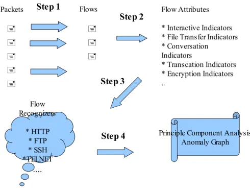
The method that is followed at this work can be viewed at four steps. To get a general view the steps are explained in a simple way. The details are explained at the following subsections.

• Packets are grouped into flows : Off line data is used at this thesis. The

details about the captured data is given at the subsection 3.2. The data is a prerecorded data that includes captured traffic by tcpdump. The recorded data is first converted into a flow record by keeping mac address information, packet performance data, application byte metrics in each audit record.

• Characteristics (attributes) are measured on each flow : Attributes mentioned

at the Annie De Montigny and Leboeufare (De Montigny and Leboeuf 2005) work are calculated and recorded.

properties. One category includes the metric values of the flow, the other one is the statistical information that is gathered through a packet inspection. With these knowledges it is aimed to define the application level definition for a flow.

• Anomaly Detection : Anomaly analysis is covered on the undefined flow

data. Undefined traffic is saved for a further statistical analysis to detect uncorrelated data from the correlated data.

The process is outlined also at Figure 3.1 in a more visual way.

 

 

 

 

Figure 3.1. Steps Through Anomaly Detection

There are some points that should be highlighted about the approach in this thesis:

• Anomaly detection method at this thesis is based on traffic characterization

which requires to derive flow characteristics. At the current work it is possible to get and analyze nearly twenty three flow metrics.

• It is completely avoided relying on port numbers or payload analysis. This

provides an alternative method to more conventional traffic categorization techniques provided by current networking tools.

Packets Flows Flow Attributes

* Interactive Indicators * File Transfer Indicators * Conversation Indicators * Transcation Indicators * Encryption Indicators .. Flow Recognizers * HTTP * FTP * SSH *TELNET ....

Principle Component Analysis Anomaly Graph

Step 1

Step 2

Step 3

• It is only examined communication patterns found at the network and

transport layers, requiring minimal information per packet to be retained.

• Patterns are identified at the 5-tuple flow granularity of TCP/UDP

communications. Therefore even sporadic malicious activities may be identified without the requirement of waiting until multiple connections can be examined.

• The flow attributes can serve as a starting point for different traffic

characterization studies. By using the same attributes but different statistical analysis more powerful techniques can be defined. The methodology also open to adding to new flow attribute additions. So defining new attributes may ease the anomaly detection process.

3.2. Processing of Captured Data

The traffic analysis process starts with a tcpdump data file which is used for extracting flow data and for gathering per packet information. There are two types of tcpdump records that was used through this thesis work. One of them is the 1999 DARPA Intrusion Detection Evaluation Data Set which was used throughout the development phase. DARPA Intrusion Detection Evaluation Data Set (DARPA 2009) includes weekly prerecorded tcpdump files for further evaluation. The data set was used for intrusion detection so it has separated clean traffic. Attack free (clean) traffic was important during the development period to detect the metric values for each flow attributes. So the first week of the dataset is used for development purposes. Second record type is the one including manually produced anomalies. These records include both abnormal traffic and a scheduled attack produced manually. These type of records are used for checking the accuracy of the work.

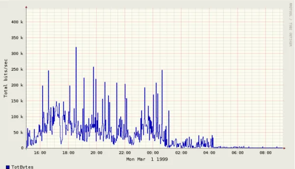
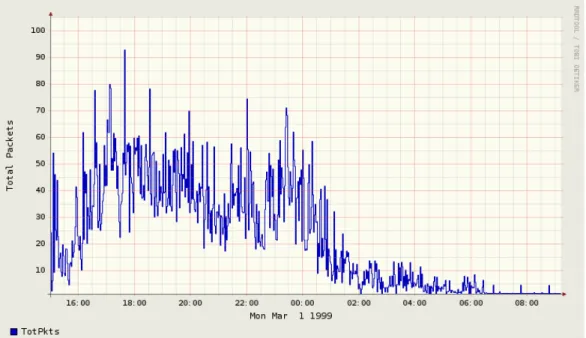
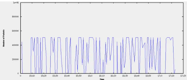
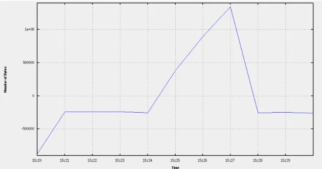
Below is the graphical and statistical representation of the week one day one record of the DARPA Intrusion Detection Evaluation Data Set:

h. File name: inside.tcpdump_w1_d1 File type: Wireshark/tcpdump/... - libpcap

File encapsulation: Ethernet Number of packets: 1492331 File size: 341027537 bytes Data size: 317150217 bytes

Capture duration: 79210.265570 seconds Start time: Mon Mar 1 15:00:05 1999 End time: Tue Mar 2 13:00:16 1999 Data rate: 4003.90 bytes/s

Data rate: 32031.22 bits/s

Average packet size: 212.52 bytes

h. represents the all available statistical information gathered from the captured file, inside.tcpdump_w1_d1 which is the name of the file created by using Tcpdump.

Following two figures give the graphical representation of the flow information for the captured file.

During the preprocessing period, the prerecorded dump file is first converted into Argus flow file. After this process flow records are written to a text file in a human readable form. The records include 5-tuple key information, direction of transaction, record start time, record last time, record total duration, transaction bytes from source to destination, transaction bytes from destination to source, application bytes from source to destination, application bytes from destination to source, packet count from source to destination, packet count from destination to source, source packets retransmitted or dropped and destination packets retransmitted or dropped for each flow.

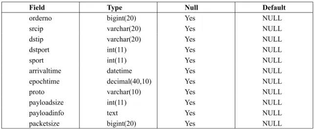
Preprocessing period also requires packet based traversing on the recorded traffic. While traversing on the recorded data, information per packets are saved. To save the packet based information database table created on MySQL database server is used. MySQL is a relational database management system (RDBMS). Because it is a fast, stable and true multi-user, multi-threaded SQL database server it is used to save packet level information. Below is the structure of the table that is used to keep whole flow packet information.

Table 3.1. Table structure for table FlowPkgTbl

Field Type Null Default

orderno bigint(20) Yes NULL

srcip varchar(20) Yes NULL

dstip varchar(20) Yes NULL

dstport int(11) Yes NULL

sport int(11) Yes NULL

arrivaltime datetime Yes NULL

epochtime decimal(40,10) Yes NULL

proto varchar(10) Yes NULL

payloadsize int(11) Yes NULL

payloadinfo text Yes NULL

packetsize bigint(20) Yes NULL

For each of the flow record, attribute values that are mentioned at the Chapter 2 are calculated. As it is mentioned some attribute metrics require packet based inspection that means packets that belong to the analyzed flow should be taken into consideration. To identify in request packets, 5-tuple key value is used from the flow information. Packets including the 5-tuple key information are queried from the FlowPkgTbl. By traversing on the result set and following the calculations mentioned at the Chapter 2, flow attributes are calculated. Packet based attribute calculation requires additional database tables usage.

3.3. Processing of Flow Data

Attribute values are used to define the flow characteristics. For each of the protocol, observed values of the flow attributes are given at the De Montigny and

Leboeuf's work (De Montigny and Leboeuf 2005). The values are added to the Appendix B. Throughout the development phase, to check the correctness of the values defined at the paper, protocol based traffic should be used, so for every application level protocol that is under consideration, specific traffic is extracted from the recorded traffic record. This is done using the racluster, Argus client. Racluster enables filtering traffic. A sample racluster command for filtering HTTP traffic and creating flow data is as

follows:

i. racluster -L0 -nr tcpdump-07-05-2009_23:25:24.dump.arg3 -s proto saddr sport dir daddr dport stime ltime dur sbytes sappbytes dappbytes dbytes spkts dpkts sloss dloss - ip and port 80 >

tcpdump-07-05-2009_23:25:24.dump.txt

This command takes tcpdump-07-05-2009_23:25:24.dump.arg3 Argus flow data as input and produces clustered readable flow information by filtering IP based traffic and port 80, that is flows with UDP, TCP or ICMP protocols with destination or source port number 80 is taken into consideration.

Another reason to use the filtered flows is the necessity of calculating threshold value for each protocol. By looking at the flow attribute values and the value ranges defined at the De Montigny and Lebouf's paper, it is only possible to produce the percentage of the relevance for each protocol. By observing the test results, a threshold value is produced for every protocol. Any match result below that percentage is marked as undefined flow for PCA.

Thresholds are calculated for each application level protocol. By using the clean data set and the filtered application level flows, match results for each protocol is calculated. By looking at the average of the collected results a general tendency at the threshold value for each protocol is calculated. Chapter 4 gives the details about the test results.

3.4. Handling Flow Attributes

Flow attributes are mainly calculated on non-empty packages. A non-empty packet is the one carrying a payload. The reason about dealing with non-empty packets is that packets carry either binary data or protocol specific commands through payload. It is clear that the size of the payload may vary depending on the capture snaplen, but the default value of using the first 60 Bytes are enough to decide about the protocol. Generally the size of the payload is used instead of the text based inspection. Depending on the protocol itself, it is seen that size of the payload can bu used for detecting some

information about flow. In addition, calculating the size is easier than inspecting the ingredients of the payload.

3.4.1. Discrete Distribution Attributes for Payload and Inter-Packet

Delay

Discrete distributions are used for inter-packet delay and packet payload length. Distribution values are especially important for packet payload length. Application protocol overhead may imply that non-empty packets are always greater or equal in length to a given minimum (due to header length). Application negotiation mechanisms may also exhibit a high frequency of packets of special sizes. Moreover, certain applications may have a preferential packet size, and completely avoid sending packets of lengths within a given range. For instance, as noted in (Hernandez-Campos, et. al. 2005), the HTTP-protocol is characterized by many short and long packets. Such characteristics are not effectively reflected by means and variances which may be sensitive to outliers. Discrete distribution attributes are therefore preferred in this work (De Montigny and Leboeuf 2005).

The payload and inter-packet delay delimiters are used as defined at the De Montigny and Leboeuf's work (De Montigny and Leboeuf 2005).

It is currently used the following bin delimiters for payload length (in bytes): j. [0-1[, [1-2[, [2-3[, [3-5[, [5-10[, [10-20[, [20-40[, [40-50[, [50-100[,

[100-180[, [180-236[, [236-269[, [269-350[, [350-450[, [450-516[, [516-549[, [549-650[, [650-1000[, [1000-1380[, [1380-1381[, [1381-1432[, [1432-1473[, [1473-inf[.

The inter-packet delays are distributed according to bins ranging from 0 to 64 second-delays. It is currently used the following bin delimiters for inter-packet delay (in seconds):

k. [0-0.000001[, [0.000001-0.0001[, [0.0001-0.001[, [0.001-0.01[, [0.01-0.1[, [0.1-1.0[, [1.0-10.0[, [10.0-64.0[, [64.0-inf[.

Below tables display a conceptual illustration.

Table 3.2. Conceptual illustration of discrete payload distribution

Payload _{45% 30% 10% 15%}

(bytes) _{[0 [1 ... [1000 [1380 [1381 ... [1473 [1500, +]}

Table 3.3. Conceptual illustration of discrete packet delay distribution

Inter-packet delay

45% 30% 10% 15%

(seconds) _{[0 [10}-6 _{[0.0001 [0.001 [0.01 [1 [10 [64, +]}

According to the Table 2.3, 45% of the packets carried no data, and another 45% of the packets were relatively big, not full size packets but big packets.

3.4.2. Conversations and Transactions

Conversation and transactions are heuristic approaches to the directionality of the whole connection. Packets are treated as a sequence of positive and negative values (the sign of each value indicates the direction of the packet) and the idea is to characterize the changes in sign. Whether they are interactive or machine-driven, applications often exhibit differences with respect to the transaction and conversation indicators.

A conversation episode in this work contains consecutive (back to back) packets in one direction followed by consecutive packets in the other direction. There is also a sustained conversation definition that is the episode containing consecutive packets in one direction, followed by consecutive packets in the opposite, and followed again by consecutive packets in the first direction (e.g. A->B, B->A, A->B).

According to the De Montigny and Leboeuf's work ALPHA, BETA and GAMMA values of a conversation is calculated as follows (De Montigny and Leboeuf 2005). Let M be the total number of empty packets in a flow, let C be the number of non-empty packets associated with a conversation, and ζ be number of non-non-empty packets associated with a sustained conversation. It is defined ALPHAconversation as the number of

non-empty packets that belong to a conversation over the total number of non-empty packets:

ALPHAconversation = _MC (3.1)

It is defined BETAconversation as the number of non-empty packets that belong to a

sustained conversation over the total of non-empty packets that belong to a conversation:

BETAconversation =

ζ C

(3.2)

Let O be the number of non-empty packets associated with a conversation and transmitted by the Originator, it is defined an indicator of symmetry in a conversational flow, GAMMAconversation as the proportion of conversation packets that are transmitted by

the originator:

GAMMAconversation = O

C

(3.3)

A similar approach is applied for the transactions. Transactions include “ping-pong” exchanges, where one packet is followed by a packet coming in the opposite direction. It is quantified this phenomenon by comparing the number of changes in sign effectively seen, with the maximum number of times a change of sign can occur, given the number of positive and negative values in that sequence.

More precisely, let ρ and η be respectively the number of positive and negative values, the maximum number of time a change in sign can occur, denoted by τ, is

τ = _2min2p_−_{p , n}1 _if p_otherwise=n (3.4)

and let δ be the number of sign changes observed, then

ALPHAtransaction = δ_τ (3.5)

is an indicator of how often “ping pong” exchanges are seen in a flow. τ is equal to 0 when the flow is unidirectional and thus ALPHAtransaction may not be defined for all

flows. ALPHAtransaction is initialized to zero by default. When ALPHAtransaction is non-zero,

a value close to 1 is a strong indicator of multiple transaction exchanges.

3.4.3. Encryption Indicators

Encryption indicators are calculated by comparing the greatest common divisor (GCD) values of payloads.

The algorithm follows an iterative process. At each step, the array of input is broken into two parts for pair wise GCD calculation, and the array to be examined in the following step will contain the GCD values that are greater than 1.

The process is interrupted if, at a given step, the count of GCDs that are greater than 1 is smaller than the count of GCDs equalled to 1. The calculation is done for each direction separately, the output gives two values:

ALPHAcipherblock gives the estimated popular GCD among payload lengths of

packets. BETAcipherblock gives the ratio of non-empty packet-payloads that are divisible by

ALPHAcipherblock.

If the GCD calculation process got interrupted due to too many pair-wise GCD equal to one, then the value for ALPHAcipherblock is equal to 1 and the value for

BETAcipherblock is set to 0.

the lengths of encrypted packets typically have a greatest common divisor different than one (Zhang and Paxson 2000).

3.4.4. Command Line and Keystroke Indicators

Command-line transmissions are larger in size and are separated by longer delays than keystrokes. The distinction between command-line and keystroke interactivity helps refine the classification process a step further. FTP command for instance can be distinguished from interactive SSH and TELNET sessions; and it is foreseen that chat sessions will be classed differently depending on the “flavour” (De Montigny and Leboeuf 2005).

For keystroke interactive indicators, a small packet is defined as a non-empty packet when carrying 60 bytes or less. The inter-arrival delays between keystrokes are taken as between 25ms (dmin) and 3000ms (dmax).

On the other hand, for command line indicators, a small packet is defined as a non-empty packet when carrying 200 bytes or less. The inter-arrival delays between keystrokes are taken as between 250ms and 30000ms.

For each direction of the flow, let Ω be the set of delays between consecutive small packets and Δ = { ω Ω, such that dmin≤ω≤dmax }, the indicator of interactive∈

inter-packet departure is defined as:

ALPHAinteractive = number of elements ∈Δ number of elements∈Ω

(3.6)

Let S be the number of small packets, let N be the number of non-empty packets, let G be the number of gaps between small packets, the indicator of interactivity based on the proportion of small packets is:

Here, a gap occurs whenever two small non-empty packets are separated by at least one packet (big or empty). The indicator of consecutive small packets is

GAMMAinteractive = S−G−1

N

(3.8)

The fourth indicator gives the proportion of small non-empty packets with respect to the total number of small packets (including empty packets). The goal with this heuristic is to penalize machine-driven applications that transmit a lot of small packets, which may however be dominated by empty control segments (i.e. TCP ACK packets without piggyback data). Thus let E be the number of empty packets, it is defined:

DELTAinteractive = S SE

(3.9)

Lastly, it is defined a fifth indicator measuring irregularity in the transmission rate of consecutive small packets. Let µ and σ be respectively the mean and standard deviation of the delays between consecutive small packets; let Λ= { ω Ω, such that ω∈

[µ-σ,µ+σ] }, then the indicator of irregularity between inter-arrival times of

∈

consecutive small packets is:

EPSILONinteractive = 1−number of elements∈Λ

number of elements∈Ω

(3.10)

3.4.5. File Transfer Indicators

From the interactive indicators, it is derived file transfer indicators. In general, a file transfer flow contains episodes of consecutive big packets transmitted within a short delay. A big packet is defined as carrying 225 or more bytes. A short inter-packet delay is 50ms or less.

number of non-empty packets, let G' be the number of gaps between big packets. Furthermore, let Ω' be the set of delays between consecutive big packets and Δ' = { ω ∈

Ω', such that ω [0, dmax] }, then the indicator of inter-packet departure during a file∈

transfer is:

ALPHAfile =

number of elements∈Δ' number of elements∈Ω '

(3.11)

The indicator of file transfer based on the proportion of big packets is defined as:

BETAfile = B N

(3.12)

and lastly, the indicator of consecutive big packets is

GAMMAfile = B−G '_N −1 (3.13)

3.5. Deriving Anomaly

According to the Lakhina, Crovella and Diot's work (Lakhina, Crovella and, Crovella 2004), number of bytes, number of packets and number of IP flow values for a flow traffic can be used to identify anomalies on the network traffic. It is required the evaluation of multivariate time series of origin-destination flow traffic defined as # of bytes, # of packets and # of IP flows. By using the subspace method (Lakhina, Crovella, and Dio 2004) it is showed that each of these traffic types reveals a different (sometimes overlapping) class of anomalies and so all three types together are important for anomaly detection.

The subspace method works by examining the time series of traffic in all OD flows simultaneously. It then separates this multivariate timer series into normal and anomalous attributes. Normal traffic behavior is determined directly from the data, as

the temporal patterns that are most common to the ensemble of OD flows. This extraction of common trends is achieved by Principal Component Analysis (Lakhina, Crovella and, Crovella 2004).

To produce the multivariate time series of a flow traffic, splitting the record is required. Rasplit, Argus client, is used for splitting the record into sub flows depending on a time interval. The time interval is chosen depending on the flow duration. Either 1 minute or 5 minute time interval values are used.

By traversing on the sub flow files, # of bytes, # of packets or # of IP flow values are calculated depending on the origin-destination pairs. A file with comma separated values (CSV) is created. The CSV file is used for creating matrix for PCA evaluation. After the PCA value is calculated, transformed data of the PCA result is graphed. It is observed that peeks at the graphs represents the anomalies at the network traffic.

CHAPTER 4

IMPLEMENTATION

This section includes the implementation details of the approach preferred in this thesis. Starting from the programming language preferred from development, class structure details and the implementation steps are explained. Python is chosen as the development programming language. A class hierarchy is constructed and implemented by using Python. The details of the class hierarchy is given as UML diagrams. By following the class structure and using the Python language, steps that should be followed for running the software is defined.

4.1. Programming Language

This thesis can be divided into two level of survey. The first level is the traffic characterization, which requires pcap file traversing to get the packet level information, operation on MySQL database tables and mathematical calculations. Second level is the PCA part which is done mainly by Octave. It is used a CSV file for Octave's princomp

function as an input. The CSV file creation requires flow splitting and traversing on the readable flow files to calculate # of values and save them to database.

It is chosen Python as the programming language for development. Python is an interpreted, object-oriented, high-level programming language with dynamic semantics. Its high-level built in data structures, combined with dynamic typing and dynamic binding, make it very attractive for rapid application development, as well as for use as a scripting or glue language to connect existing components together. Python's simple, easy to learn syntax emphasizes readability and therefore reduces the cost of program

maintenance. Python supports modules and packages, which encourages program modularity and code reuse. The Python interpreter and the extensive standard library are available in source or binary form without charge for all major platforms, and can be freely distributed (Python 2009). Python is also actively used by penetration testers, vulnerability researchers and information security practitioners.

Python's Scapy (Scapy 2009) module is used to decode packets from pcap files and analyze them according to their header information. Scapy is a powerful interactive packet manipulation program. It is able to forge or decode packets of a wide number of protocols, send them on the wire, capture them, match requests and replies, and much more. Scapy is mainly used for traversing through the prerecorded network traffic via tcpdump and get IP level information from packets for saving them to the database.

By using Scapy it is possible to get the source IP address, source port number, destination IP address, destination port number, packet size, payload ingredients and payload size, capture time and protocol information from each packet. Capture time is valuable for calculating jitter. Payload size is important for detecting the non-empty packets. The rest of the information that is 5-tuple key also, is used to understand what flows they belong to.

4.2. Class Structure

4.2.1. Flow Object