Edited by: Marcos Egea-Cortines, Universidad Politécnica de Cartagena, Spain Reviewed by: Ankush Prashar, Newcastle University, UK Alan Gay, Aberystwyth University, UK *Correspondence: Carlos Poblete-Echeverría [email protected] Gustavo A. Lobos [email protected] Specialty section: This article was submitted to Technical Advances in Plant Science, a section of the journal Frontiers in Plant Science Received:17 July 2016 Accepted:16 December 2016 Published:09 January 2017 Citation: Lobos GA and Poblete-Echeverría C (2017) Spectral Knowledge (SK-UTALCA): Software for Exploratory Analysis of High-Resolution Spectral Reflectance Data on Plant Breeding. Front. Plant Sci. 7:1996. doi: 10.3389/fpls.2016.01996
Spectral Knowledge (SK-UTALCA):
Software for Exploratory Analysis of
High-Resolution Spectral
Reflectance Data on Plant Breeding
Gustavo A. Lobos1* and Carlos Poblete-Echeverría2, 3*
1Plant Breeding and Phenomic Center, Facultad de Ciencias Agrarias, PIEI Adaptación de la Agricultura al Cambio Climático, Universidad de Talca, Talca, Chile,2Escuela de Agronomía, Pontificia Universidad Católica de Valparaíso, Quillota, Chile, 3Department of Viticulture and Oenology, Faculty of AgriSciences, Stellenbosch University, Matieland, South Africa
This article describes public, free software that provides efficient exploratory analysis of high-resolution spectral reflectance data. Spectral reflectance data can suffer from problems such as poor signal to noise ratios in various wavebands or invalid measurements due to changes in incoming solar radiation or operator fatigue leading to poor orientation of sensors. Thus, exploratory data analysis is essential to identify appropriate data for further analyses. This software overcomes the problem that analysis tools such as Excel are cumbersome to use for the high number of wavelengths and samples typically acquired in these studies. The software, Spectral Knowledge (SK-UTALCA), was initially developed for plant breeding, but it is also suitable for other studies such as precision agriculture, crop protection, ecophysiology plant nutrition, and soil fertility. Various spectral reflectance indices (SRIs) are often used to relate crop characteristics to spectral data and the software is loaded with 255 SRIs which can be applied quickly to the data. This article describes the architecture and functions of SK-UTALCA and the features of the data that led to the development of each of its modules.
Keywords: phenotyping, phenomic, scan, wavelength, noise, outlier, spectral reflectance index (SRI), collinearity
INTRODUCTION
The responses of any living organism are ultimately controlled by genes (G), but the expression of these are modulated in several ways, partly because of the action of other genes, and the complex interaction between them, but mostly in response to the environment (E) where the plant grows and develops (GxE interaction). Gene sequencing is becoming more routine, economical, and fast, but for proper analysis and interpretation of the information an adequate phenotypic characterization is essential, even though it poses one of the greatest difficulties (Lörz and Wenzel, 2005; Finkel, 2009; Lobos et al., 2014; Estrada et al., 2015).
Progress in science and technology have made it possible to study different processes involved in multiple areas of knowledge. In agronomy and biological sciences, sensors, and instrumentation have been developed to characterize the behavior of a particular organism, or a group of them, under a specific environmental condition or situation.
Currently, equipment, techniques, and analyses are available that have proved helpful in characterizing the phenotype (phenotyping), and in the case of remote sensing, quick and high predictive power (Lobos and Hancock, 2015; Camargo and Lobos, 2016).
Among the available remote sensing tools, spectrometers, or spectroradiometers mainly exploit the principle of quantifying the proportion of reflected radiation by an object relative to the incident radiation (Borengasser et al., 2008). Reflectance (graphically represented by the spectral signature) is related to the absorption and transmission of each wavelength, thus representing plant status under ambient or experimental conditions (Garriga et al., 2014). For example, compared to a senescing plant, a healthy one should absorbs more in the visible (blue and red light) and reflect more in the near infrared range.
Nowadays plant reflectance can be measured from space by satellites (with certain limitations on interpretation due to pixel resolution) or from the troposphere by manned and unmanned aerial vehicles (problems related to the number and resolution of the spectrum bands;Araus and Cairns, 2014). Equipment used on the ground covers a wider range of the spectrum, with a better resolution. The most modern devices not only measure into the near infrared region (700–1300 nm; NIR), but also from the ultraviolet (∼200 nm) up to the short wavelength infrared (∼2500 nm) (Cabrera-Bosquet et al., 2012). This high-resolution technology allows examination of plants beyond the 1000 nm region of the spectrum, with great potential for phenotype prediction (Garbulsky et al., 2011; White et al., 2012; Araus and Cairns, 2014; Lobos et al., 2014).
Several critical issues for making good reflectance measurements in the field have been reported in the literature (e.g., Curtiss and Goetz, 1994; Milton et al., 1995; Salisbury, 1998; Schaepman, 1998; Curtiss and Goetz, 2001). Independent of the equipment used on the ground, a correct measurement of the reflectance in the field is mandatory. Ideally, measurements should be restricted to clear sky conditions, performing a radiometric calibration every 10–15 min to limit variations in reflectance induced by changes in the angle of the sun, and taking in account basic but important considerations such as maintaining the same orientation, angle, and distance to the canopy on each assessed plot or ensuring dark colored clothing for the operators. Although instrument settings vary among brands and models, a number of steps should be followed to optimized data capture. The equipment should be turned on in advance to allow the device to equilibrate with the ambient temperature, the integration time for a single scan or sample needs to be defined (maximizing sensitivity, but avoiding saturation), the number of scans per sample or samples per plot and the convenience of averaging them before data processing should be determined, and the exact sequence for checking darks and standards recommended by the manufacturer needs to be ascertained.
In general, due to its simplicity and ability to forecast several phenotypic characteristics, reflectance is used to calculate “Spectral Reflectance Indices” (SRIs) (Lobos and Hancock, 2015). SRIs are based on relationships between wavelengths or spectrum bands, usually designed to be relatively immune to changes in solar radiation between measurements, relating them quantitatively to changes in plant phenotype (Mullan, 2012). Today there are hundreds of SRIs proposed to estimate different traits (e.g., leaf area index, yield, gas exchange, fluorescence, pigment content, plant water status, carbon isotopic
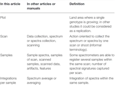
TABLE 1 | Nomenclature related to spectrometer data collection.
In this article In other articles or manuals
Definition
Plot Land area where a single
genotype is growing; in other studies it could be considered as a replication.
Scan Data collection, spectrum or spectra collection, scanning
Action oriented to collect the spectrum or spectra by one scan or shoot (informal terminology). Samples Sample spectra, samples
of scan, scanned samples, scanned data, artifacts, features
Some spectrometers are able to register several samples within the same scan; number of spectral signatures captured per scan.
Integrations per sample
Spectrum average or averaging
Integration of spectra within the same sample.
discrimination, etc.) but because of the lack of tools capable of assessing several SRIs at the same time, most of the published works focus on a small percentage of them (e.g., SR, NDVI, WI, NDWI, PRI, SAVI, etc.).
In breeding programs, there is a need to regularly evaluate hundreds or thousands of genotypes in a short time. Therefore, due to the time and cost involved breeders have not been able to perform a thorough phenotypic characterization of the material, limiting their evaluations to the yield, its components and some others traits that are relatively easy to assess (Kipp et al., 2014; Lobos and Hancock, 2015; Camargo and Lobos, 2016). With the emergence of phenomics, which is the acquisition of high-dimensional phenotypic data (high-throughput phenotyping) for characterization of the phenotype of organisms in a multidimensional manner (Houle et al., 2010; Kipp et al., 2014), measurements that used to take weeks or months can now be performed in a few hours (White et al., 2012; Lobos and Hancock, 2015). The implementation of phenomics in plant breeding programs is relatively new, and is an area where more development is likely to be needed (Lobos and Hancock, 2015).
For a correct interpretation of spectral reflectance data, it is essential to have reliable and representative information, especially when it comes from field measurements. The use of reflectance data in breeding programs has several advantages but probably the major problem is the amount of data originated by the numbers of wavelengths and genotypes assessed. If the reflectance data is analyzed in a conventional way (e.g., Excel files), the detection of measurement errors, the study of the spectral noise (originating from absorption by environmental compounds such as water or CO2) or the relationship between a specific wavelength and a response variable become difficult or subjective. Nevertheless, as far as we are aware there is currently no free software available that allows detailed exploratory analysis of high-resolution spectral reflectance data. Therefore, the aim of this article is to present an overview of the architecture and functions of Spectral Knowledge (SK-UTALCA), software that has been specially developed for exploratory analysis of
high-resolution spectral reflectance data, with applications in plant breeding research and also in many other fields.
Due to the broad nomenclature related to spectral measurements, some definitions are given in order to facilitate the understanding of this article and software (Table 1).
MAIN SK-UTALCA ARCHITECTURE AND
FUNCTIONALITIES
Spectral Knowledge (SK-UTALCA) is a software package developed in MatlabR and is available compiled for use in a
Windows 64-bit environment from a download link or as source
code in supplementary material. This program allows, in an efficient and versatile manner, two types of actions: (i) cleaning of the data matrix by studying the spectral noise, and detecting within- and between- measurement errors; and (ii) application of a preliminary analysis of wavelength collinearity, and the detection of wavelengths or SRIs related to a response variable (Table 2).
After X and Y are loaded, the user can perform any main command, without a specific order. At the same time, each analysis can be run considering the previous exploration (Run from current data) or from the original data (loaded as X) (Run from original data). On each section of the cleaning data matrix
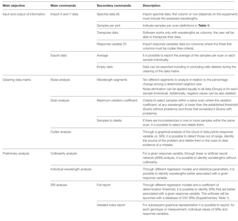
TABLE 2 | Main SK-UTALCA functionalities according to the program menu.
Main objective Main commands Secondary commands Description
Input and output of information Import X and Y data Spectral data (X) Import spectral data: first column or row (depends on the equipment) must include the assessed wavelengths.
Samples per plot Indicate samples per scan (definitions inTable 1).
Transpose data Software works only with wavelengths as columns; the user will be able to transpose their data.
Response variable (Y) Import response variables data (on columns) where the three first columns must be codes (free criteria).
Export data Average It is possible to export the average of the samples per scan or each sample individually.
Empty data Data can be exported including or excluding cells deleted during the cleaning of the data matrix.
Cleaning data matrix Noise analysis Wavelength segments Ten different segments to analyze in relation to the percentage change among a determined neighbor size.
Noise elimination can be applied equally to all data (Group) or for each sample (Individual). Additionally, negative values can be also deleted. Scan analysis Maximum variation coefficient Criteria to select samples within a same scan where the variation
coefficient, at any wavelength, is lower than the established threshold (Scans without problems) and those that exceeded it (Scans with problems).
Samples to delete If there are inconsistencies in one or more samples within the same scan, it is possible to select and delete them.
Outlier analysis Through a graphical analysis of the cloud of data points (response variable vs. SRI), it is possible to detect those out of range, identify the source of the problem and delete them in the case of clear evidence of a mistake.
Preliminary analysis Collinearity analysis For a given response variable, through linear or artificial neural network (ANN) analysis, it is possible to identify wavelengths without collinearity.
Individual wavelength analysis Through different regression models and statistical parameters, it is possible to identify wavelengths better associated with a given response variable.
SRI analysis Full report Through different regression models and a coefficient of
determination threshold, it is possible to identify SRIs that are better associated with a given response variable. The software will be launched with a database of 255 SRIs (Supplementary Table 1). Detailed index report For subsequent graphical representation it is possible to export, for
each genotype or measurement, individual values of SRIs and response variables.
or the preliminary analysis, the user will be able to export the analyzed information (csv format).
Main Menu (Data Set)
In the main menu, users are required to load the spectral reflectance data [Spectral data (x)]. The first step in the use of SK-UTALCA software is to load the data set in Microsoft Excel format (xlsx format). To read the spectral data it is necessary to indicate the number of samples taken in each plot (Samples per plot). Depending on the equipment used, reflectance data is organized in columns or rows. In the software, the spectral bands need to be located in columns and the spectral data in rows (it is possible to use the “Transpose data” option to relocate the data set as needed). The first wavelength measured must be in the second column (the first column is for codification purposes and depends only on the user).
The second file needed (xlsx format) contains the values for the independent variables [Response variables (y)] for each plot. In this case, the spreadsheet must consider three codification columns and the first variable should be allocated to the fourth column.
The software has no limitation on the number of spectral data points (wavelengths or measurements) or response variables.
Noise Analysis
This first filter removes the spectral noise originated by the natural presence of certain elements in the atmosphere, such as water and carbon dioxide, which absorb specific wavelengths (Salisbury, 1998; Curtiss and Goetz, 2001; Psomas et al., 2005; Ma and Chen, 2006; Clevers et al., 2008). Researchers who screen hundreds or thousands of genotypes under field conditions usually consider at least three or four spectral samples per plot, generating a matrix of data that makes it difficult to objectively select the noise segment(s) for deletion. Furthermore, spreadsheet graphical options are usually restricted to a maximum number of data series per chart (e.g., ∼255 in Excel for Windows or Mac), so there is no easy way to take a decision based on this tool. For this reason, for breeding purposes, conventional visual noise elimination is not a real alternative, restricting the criteria to the assumption of arbitrary limits, usually following thresholds from a third person or related articles.
With this module, it will be possible to analyze the spectral noise by considering up to ten independent segments. This will allow the user to set up different criteria in each segment, being more or less strict depending on the wavelengths analyzed, the data collected or previous knowledge. To apply the filter on each spectral signature, it is necessary to indicate the lower and upper limit for each segment (Wavelength segments), the maximum accepted percentage of variations (%) between two neighboring wavelengths, and the number of neighbors (N size) where the previous condition is found consecutively. The graphic window will show red crosses where the first criterion is satisfied and black ones where both have been met, this last condition determining where the software will perform the cleaning.
However, an objective selection is not the only important aspect of spectral noise. During the day there are environmental
changes (e.g., relative humidity) that not only affect the magnitude of each problematic wavelength, but also the number of wavelengths involved. For instance, measurements performed under conditions of higher relative humidity (usually before midday) produce wider noise segments beyond 1000 nm; if the determination of the number of wavelengths to eliminate considers measurements across the whole day, the noise edges will be established by genotypes evaluated early in the day (broader noise segments), risking the loss of important spectral information from those assessed under lower relative humidity (usually after midday) and therefore possessing narrower noise segments.
Because of this, after the noise selection criteria (% and N Size) are established, the user has an opportunity to filter by considering all the measurements as one group (Group) or as individual scans (Individual). When thegroup filter is selected in a specific segment, the program analyzes each sample where the selection criteria are met, identifying the minor and major wavelengths that have problems in the spectral data file, and uses these two wavelengths to eliminate the noise from each sample uniformly. This is very similar to what is done visually, but with an objective approach. For theindividual option, each sample will be filtered independently from the others, rescuing important information for modeling, or the use of SRIs.
Scan Analysis
In this module, the user will be able to analyze, identify and correct inconsistencies between spectral signatures from the same scan or plot, a problem that is often unnoticed. In general, for simplicity or to dilute any errors generated while collecting the data, there is a tendency to average samples within the same scan, which most of the time is done without any deeper analysis. As mentioned before, this should not be a complication when the data analysis considers a few measurements, but in breeding programs this search would be time consuming.
There are several aspects influencing the homogeneity between samples within the same scan, especially if the measurements were performed under field conditions. Unnoticed modification of the measurement angle during plot screening is probably the main source of variability. In practical terms it is difficult to maintain the exact angle of measurement, even for a few seconds (hand steadiness of the operator, distractions, or fatigue); each sample is derived from several integrations, usually more than 10, so the chance of making a mistake is not uncommon. When a plot is screened, it can be performed by keeping the fiber aimed at a single point (lower variability and representation) or across several plants (higher representation but greater variability); when the second option is taken, the chances of integrating other materials into a single scan or sample (e.g., soil, weeds, or air) are increased, and also enhanced by changes in measurement angles. Other considerations such as the effect of the wind speed or turbulence on the measured surface would be detected.
The user needs to set up theMaximum variation coefficient
accepted for the samples belonging to the same scan. The software will find the scans where the limit is exceeded, at any wavelength, and this will be reported in theScans with problems
section. The samples that need to be checked can be individually analyzed on the graphical window, where it is possible to visualize all the samples in a single graph, identifying (zooming in and out) and deleting those spectral signatures with problems.
It is important to mention that the samples selected with problems within a same scan, do not necessarily need to be modified. This decision will depend on the magnitude of the differences between samples and the number of wavelengths involved. In cases where the user decides to intervene in a scan, it is possible to select and delete one or more samples from the
Samples to deletesection.
Outlier Analysis
This third filter is designed for rapid identification of problems associated with inconsistencies within spectral data. When outlier data is found, it will be necessary to evaluate the permanence of these in the data matrix.
Because of the high number of genotypes and samples per scan, it is difficult to identify data points that do not follow the general trends. Field experience has proven that is common to find small clouds of data whose main source of error comes
from the calibration process. For example, the sun’s movement throughout the day requires calibrations to be performed every 10–15 min. Due to distractions or tiredness during long working hours, the calibration can be forgotten, generating differences in the sun’s incidence angle and therefore variations in the reflectance readings. Another form of user error, although less common and related to specific devices, may occur if the user has left the mouse cursor on one of the calibration icons (optimization, dark current, or white reference), performing an unconscious and incomplete calibration with a random click and thus generating undetectable reading errors.
In this module, it is possible to integrate a visual analysis of the reflectance and the response variable data at the same time. The user has four graphs to explore outlier information, evaluating different SRIs, and traits. In this section, it is also possible toEdit
each graph, selecting data that need to be removed from the data matrix.
For these actions, the software will average the samples per scan to generate each SRI. This is important because the user should check the Noise Analysis and Scan Analysis modules first.
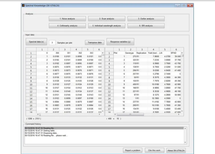
FIGURE 1 | Main screen divided horizontally into three sections: analysis, input data, and command history.Screen shows loaded databases (spectral and response variable data files); thetranspose dataoption is also available for the spectral matrix.
FIGURE 2 | Example of noise analysis showing 400 scans (x 3 samples ea.) prior to (A)and after(B)the noise filter was applied. On both windows, red crosses (top) show where the maximum percentage of variations was exceeded and black crosses (top) where both criteria (% and the number of neighbors) were detected.
Collinearity Analysis
Collinearity or multicollinearity is a problem in regression analysis where the predictor variables “X” are themselves highly correlated (Draper and Smith, 2003). With the use of high-resolution spectral reflectance data, the collinearity problem is inherent to the data collection method employed because several wavelengths are highly correlated. If the goal is to understand how several predictor variables impact on a specific response variable “Y,” the collinearity is a big issue. Therefore, depending on the modeler’s interest, it may be necessary to implement a collinearity analysis before construction of complex models (e.g., multilinear regression model).
In this module, the user can identify wavelengths that deliver the same predictive information for a given response variable, keeping only those that best explain it. This analysis can be performed (collinearity test setting) bylinear regression, indicating the threshold coefficient of determination (R square cutoff), or through Artificial Neural Networks (ANN), considering a training process by Levenberg-Marquardt (trainlm), and Mean Squared Error (MSE) as a performance indicator. Depending on the data matrix and computer performance, the non-linear approach (ANN) could take several minutes or hours.
Individual Wavelength Analysis
For the construction of new SRIs and regression models, it would be desirable to know the degree of dependency between individual wavelengths and the response variable. In this module, the researcher can study the behavior of each wavelength relative to each variable under study, considering one, or more of the following models: (1) Polynomial 1:y=p1·x+p2 (2) Polynomial 2:y=p1·x2+p2·x+p3 (3) Weibull:y=p1·p2·x(p2−1)·e(−p1·xp2) (4) Exponential:y=p1·e(p2·x) (5) Power:y=p1+p2·x(p3) (6) Logarithmic:y=p1·ln(x)+p2
For this analysis, the user can select different statistics to sort the results (adjusted and non-adjusted determination coefficient, root mean squared error, sum of squares due to errors, and degree of freedom). It is also necessary to set up a minimum or maximum value for the selected statistics in order to export just those results (Values above or below). The exported file will show, for each wavelength, the statistics values for the selected model(s) where those minimum or maximum values were met.
This module and the following one (SRI analysis) work with sample averages, forcing the user to perform a deep preliminary analysis, thus avoiding any error in the data matrix.
Spectral Reflectance Index (SRI) Analysis
The implementation of concatenate formulas in spreadsheets is helpful for automating time-consuming procedures. However, due to the number of scans, samples per scans, measured wavelengths, evaluated response variables, and tested SRIs, the physical size of the resulting spreadsheets (several MB) implies the need for high performance computers.
By evaluating the same regression models reviewed with the previous function, the user will be able to identify the SRIs (initially 255: Jordan, 1969; Rouse et al., 1973; Rouse, 1974; Tucker, 1979; Hardisky et al., 1983; Guyot and Baret, 1988;
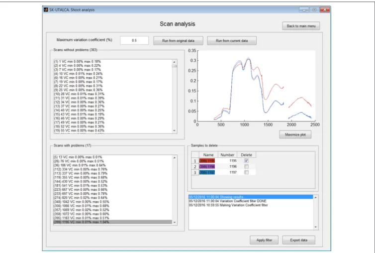
FIGURE 3 | Example of scan analysis.The software divided the scans or plots between those that did not surpass the maximum accepted variation coefficient (Scans without problems) and those where it was exceeded (Scans with problems). Scan 399 was selected, and its first sample (red) was identified for deletion (Apply filter).
Guyot et al., 1988; Huete, 1988; Baret et al., 1989; Clevers, 1989; Curran, 1989; Hunt and Rock, 1989; Major et al., 1990; Barnes et al., 1992, 2000; Chappelle et al., 1992; Gamon et al., 1992; Peñuelas et al., 1993a,b, 1994, 1995, 1997; Vogelmann et al., 1993; Carter, 1994; Gitelson and Merzlyak, 1994, 1997; McMurtrey et al., 1994; Qi et al., 1994; Roujean and Breon, 1995; Smith et al., 1995; Chen, 1996; Chen and Cihlar, 1996; Filella et al., 1996; Fourty et al., 1996; Gao, 1996; Ma et al., 1996; Rondeaux et al., 1996; Huete et al., 1997; van Deventer et al., 1997; Blackburn, 1998, 1999; Datt, 1998, 1999; Merton, 1998; Peñuelas and Filella, 1998; Gamon and Surfus, 1999; Gitelson et al., 1999, 2001, 2003, 2005, 2006; Merzlyak et al., 1999; Peñuelas and Inoue, 1999; Daughtry et al., 2000; Marshak et al., 2000; Thenkabail et al., 2000; Broge and Leblanc, 2001; Raun et al., 2001; Zarco-Tejada et al., 2001, 2003a,b, 2005; Broge and Mortensen, 2002; Haboudane et al., 2002, 2004; Read et al., 2002; Serrano et al., 2002; Sims and Gamon, 2002; Gupta et al., 2003; Hansen and Schjoerring, 2003; Steddom et al., 2003; Viña, 2003; Dash and Curran, 2004; Gandia et al., 2004; Le Maire et al., 2004, 2008; Schlemmer et al., 2005; Zhao et al., 2005; Vincini et al., 2006; Babar et al., 2006a,b; Mirik et al., 2006a,b; Inoue et al., 2007,
2008; Prasad et al., 2007; Rodríguez-Pérez et al., 2007; Zhu et al., 2007; Rama Rao et al., 2008; White et al., 2008; Wu et al., 2008a,b; Richter et al., 2009; Serbin et al., 2009; Stroppiana et al., 2009; Yañez et al., 2009; Dzikiti et al., 2010; Herrmann et al., 2010; Mistele and Schmidhalter, 2010; Yao et al., 2010, 2011; Garrity et al., 2011; Hernández-Clemente et al., 2011; Main et al., 2011; Pimstein et al., 2011; Tian et al., 2011, 2014; Winterhalter et al., 2011; Wang et al., 2011a,b) having the higher adjusted coefficients of determination (Adj. RSquare values above) in relation to a response variable. Internally, the software will select all combinations (regression model, SRI, and response variable) where the adjusted coefficient of determination was reached. The
Export dataoption will generate a report that includes all the statistics analyzed in the previous function for the best-evaluated regression model and for each one (in the case that more than two were tested).
For publication purposes this module also includes an exportableDetailed index report, where it is possible to select specific SRIs and response variables. The report will include the SRI and variable values for each of the measurements, allowing the user to create XY graphs.
FIGURE 4 | Example of outlier analysis showing four scatterplot graphs (NDVI, SR, PRI and WI vs. Yield) (A).Using theEditfunction, NDVI vs. Yield was used to select scans with NDVI values below 0.31(B)for deletion(C).
FIGURE 5 | Example of collinearity analysis for deletion of wavelengths delivering the same predictive information for Yield.The analysis, considering a linear regression method (R square cutoff=0.95), selected 131 wavelengths without collinearity.
OPERATIONAL EXAMPLES OF SK-UTALCA
Testing Data Sets
During the 2011/12 growing season, 386 genotypes of wheat (Triticum spp.L.) from different breeding programs (INIA-Chile,
INIA-Uruguay and CIMMYT) were assessed under three water regimens (fully irrigated, mild water deficit and severe water deficit). This trial was established at Santa Rosa Experimental Station (36◦ 32′ S, 71◦ 55′ W; 217 m.a.s.l.), Regional Research Center INIA Quilamapu (Chillán, VIII Region, Chile),
FIGURE 6 | Example of the individual wavelength analysis module.The relationships were searched by considering Yield and a coefficient of determination higher than 0.3(A). Results were plotted for visual analysis(B)and exported to a spreadsheet(C).
considering an alpha-lattice design (386 genotypes + 2 cvs. replicated seven times to assess field variability) and two replications.
Reflectance measurements were performed using a portable spectroradiometer (FieldSpecR 3 Jr, ASD Inc., Boulder, CO,
USA) (350–2500 nm), between 12:00 and 16:00 h, on clear days (solar radiation higher than 800 Wm−2). Prior to the first measurement and every 15 min, the equipment was calibrated using a field reference panel (Spectralon, ASD Inc., Boulder, CO, USA). The equipment was configured to read three samples per scan. Each plot (genotype) was scanned once.
A detailed methodology can be found in Lobos et al. (2014). For purposes of this article, only one environment (fully irrigated), one phenological stage (grain filling) and one replicate will be considered.
Data Analysis
In this section, we highlight some of the key results of the analysis performed using the SK-UTALCA software.
Setting Up
Prior to analysis the user needs to: (i) load the spectral data file (denoted as “x”); (ii) load the response variable(s) file (denoted as “y”); and (iii) define the number of samples per scan (in this case three). Wavelengths need to be placed in columns and samples in rows; thetranspose datafunction is available.
The file format for the spectra (Genotype, Wavelength1,
Wavelength2, Wavelength3, ... Wavelengthn) and the response variables (Plot, Genotype, Replication, Variable1, Variable2,...
Variablen) are presented inFigure 1. If for any reason the user
realizes that there are missing plots (no spectral information) before the spectral data is uploaded, keeping in mind the sample number per scan, those rows can be left empty. If calibration data is among the spectral data output from the spectrometer, it should be removed prior to uploading the reflectance data (x).
Once the data has been loaded into the software and the wavelengths are arranged into columns, it is possible to start the analysis.
Noise Analysis
To apply this filter it is necessary to indicate the wavelength segment for analysis, the cutting criteria (GrouporIndividual), the maximum percentage of variations accepted (%), and the number of neighbors (N size). The selection of each wavelength segment and the criteria for each one (% and N Size) will depend on the user experience and the environmental conditions where the measurements were taken; for example, noise at 1800– 1950 nm and 2350–2500 nm is usually wider and stronger than at 1300–1400 nm, so the criteria should consider higher values of%
andN Sizefor the first two segments. In this operational example, the filter was applied to the whole spectral range (350–2500 nm) considering a group filter, with five wavelengths asN sizeand a maximum accepted variation among them of 20%.Figure 2
shows the results prior to (A) and after (B) the filter was applied. In this case, the filter was able to detect two main noise zones from 1833 to 1935 nm and from 2422 to 2500 nm.
Scan Analysis
The Scan analysis module allows detection of abnormal variations among samples within the same scan. In this operational example, the Scan analysis was applied using the
FIGURE 7 | Example of the SRI analysis module.Three regression models were selected to search for SRI and response variables with a minimum adjusted coefficient of determination of 0.25(A). The exported file shows the adjusted coefficient of determination for the best approximation (Best) and for each selected regression model(B). When a detailed report is required(C), the SRI value for each scan is calculated automatically(D).
functionRun from the current data, that is to say, considering the results obtained using previous filter (without spectral noise). TheMaximum variation coefficientwas set at 0.5%. The software was able to select 383 scans or plots without problems and 17 where the threshold was exceeded (5, 26, 36, 112–113, 119, 144, 181, 223, 233, 274, 348, 356–358, 395, and 399). In the
Figure 3, scan or plot 399 is graphed, and the first sample (1195 on red) was selected for deletion. This result could be an indicator of a measurement problem associated with the operator (modification of the measurement angle) or external conditions (e.g., wind speed) during the first sample integrations. In case of all samples from a specific scan need to be deleted, the software will maintain this scan as empty rows, avoiding problems in further analyses.
Outlier Analysis
This module is a simple and exploratory analysis to identify outlier scans, allowing the user to detect field measurement problems (e.g., calibration). Four scatterplot graphs will show the relationship between any SRI available on the software database
and the loaded response variables. If a problem is detected, it is possible to use the Edit option to manually remove the samples. In this operational example, the relationship between NDVI and Yield was used to inspect the possible outlier samples.
Figure 4Ashows how different SRIs (NDVI, SR, PRI, and WI) can generate different data distributions, helping the user in cases where problems are not so evident; on the top left graph (NDVI vs. Yield) two clouds of data points can be identified, divided at the NDVI value of 0.31.
Once the information from the smaller data cloud was analyzed (NDVI < 0.31), it was evident that the data set
corresponded to 96 contiguous scans or plots (104–200), suggesting that there were problems associated with the measurement. When information from the spectrometer was checked, it was concluded that the operator had skipped one calibration. It is always important to check the pertinence of negative SRI values because they are probably related to measurement errors.
After identification of the origin of a particular problem, any graph can be selected for editing. In this example (NDVI vs.
Yield), the scan with the problem can be selected (Figure 4B) and deleted (Figure 4C).
Collinearity Analysis
Using linear regression or ANN, the collinearity analysis module identifies wavelengths that delivering the same predictive information for a given response variable, keeping only those that best explain it. In this operational example, collinearity analysis was applied by considering the results obtained from the scan analysis (Run from current data), with Yield being the response variable in the linear regression (R square cutoff =
0.95). Results of this analysis found 131 wavelengths without collinearity (Figure 5).
Individual Wavelength Analysis
In this module it is possible to assess the relationship of individual wavelengths and a given response variable. Three regression models were selected (Polynomial 1 and 2, and Exponential) to search for wavelengths with determination coefficientsabove
0.3 in relation to Yield (Figure 6A). If the user selectsPlot all results, a graph will show the wavelengths below and above the determination coefficient cutoff (Figure 6B). These results can be exported to a spreadsheet; for each selected regression model, only wavelengths where the chosen statistic surpassed the cutoff will be shown (Figure 6C). In this operational example, there were three groups of wavelengths with determination coefficients above the threshold: 733–1139, 1409–1815, and 1936–2421 nm.
Spectral Reflectance Index (SRI) Analysis
As in the previous module, when different regression models were considered, SRI analysis has the option to evaluate the relationship between all loaded response variables and all SRIs available in the software database. For this example, three regression models were selected (Polynomial 1 and 2, and Exponential) to search the SRIs and response variables with an adjusted determination coefficient higher than 0.25 (Figure 7A). When Export data is selected, all relationships with adjusted determination coefficients higher than 0.25 will be reported (Figure 7B); the results, which are organized according to the loaded variables (column A) and SRIs (column B), show which regression model had the highest determination coefficient (Best) for each SRI, as well as its statistics [adjusted and non-adjusted determination coefficient, root mean squared error (RMSE), sum of squares due to errors (SSE) and degree of freedom (DFE)] (columns C–H). The results for each evaluated regression model are also described (Polynomial 1: columns I–M;Polynomial 2: columns N–R, and so on). In this screen example, the adjusted R2 varied between 0.257 (Datt 850;710;680) and 0.406 (DLAI 1725;970), with these SRIs having the highest and lowest RMSEs, respectively (Figure 7B).
The selection ofOpen selection dialog(Detailed index report) enables the user to select specific SRIs and response variables for figure elaboration (Index report,Figure 7C). In this operational example, three SRIs (AI, BI, and CI) and one response variable (Yield) were selected. The SRI value for each scan or plot is given
(Figure 7D) so the user can generate XY scatter plots for each tested SRI (X) and response variable (Y).
CONCLUSIONS
Spectral Knowledge (SK-UTALCA) is a software package that allows an easy and fast exploratory analysis of high-resolution spectral reflectance data, providing the user with tools to detect measurement problems and the generation of key information for later modeling. SK-UTALCA is especially useful for plant breeding or any other research area where the number of measurements (big data files) involves long working hours that increase the risk of making involuntarily mistakes. This freely-available software is the result of several years of measurements and analysis of spectral data oriented toward the prediction of traits in plant breeding.
AUTHOR CONTRIBUTIONS
GL, CP-E contributed equally toward the intellectual input into the final version of this paper, including development of the software, data analysis, interpreting, and discussion of the results, and writing and editing the manuscript.
ACKNOWLEDGMENTS
This work was supported and financed by the research program “Adaptation of Agriculture to Climate Change (A2C2),” “Nucleo Científico Multidisciplinario” and the “Vicerrectoría de Innovación, Desarrollo y Transferencia Tecnológica (VIDTT)” from Universidad de Talca. We also received significant funds from the National Commission for Scientific and Technological Research CONICYT (FONDEF IDEA 14I10106 and FONDECYT N◦11130601). We would like to express our gratitude to Sebastian Romero, Félix Estrada, Miguel Garriga, and especially to Alejandro Escobar for continued technical assistance in field experiments and laboratory analysis. We thank also Rodrigo Aguilar and Felipe Ojeda for their outstanding programming work, Genberries Ltda. for equipment support, and Ivan Matus (INIA- Chile) for genetic material and trial maintenance. Finally, our special gratitude goes to Greg Matyjewicz (ASD Inc., Boulder, CO, USA) for technical definitions and valuable discussion.
SUPPLEMENTARY MATERIAL
The Supplementary Material for this article can be found online at: http://journal.frontiersin.org/article/10.3389/fpls.2016. 01996/full#supplementary-material
Software Availability
The compiled version of the software will be available for free downloading at http://www.fenomica.utalca.cl/ and source code is available as Supplementary Material.
REFERENCES
Araus, J. L., and Cairns, J. E. (2014). Field high-throughput phenotyping:
the new crop breeding frontier. Trends Plant Sci. 19, 52–61.
doi: 10.1016/j.tplants.2013.09.008
Babar, M. A., Reynolds, M. P., van Ginkel, M., Klatt, A. R., Raun, W. R., and Stone, M. L (2006a). Spectral reflectance indices as a potential indirect
selection criteria for wheat yield under irrigation. Crop Sci. 46, 578–588.
doi: 10.2135/cropsci2005.0059
Babar, M. A., Reynolds, M. P., Van Ginkel, M., Klatt, A. R., Raun, W. R., and Stone, M. L. (2006b). Spectral reflectance to estimate genetic variation for
in-season biomass, leaf chlorophyll, and canopy temperature in wheat.Crop Sci.
46, 1046–1057. doi: 10.2135/cropsci2005.0211
Baret, F., Guyot, G., and Major, D. J. (1989). “TSAVI: a vegetation index which
minimizes soil brightness effects on LAI and APAR estimation,” inProceeding of
the 1989 International Geoscience and Remote Sensing Symposium (IGARSS ’89) and the 12th Canadian Symposium on Remote Sensing (Vancouver, BC), 1355–1358.
Barnes, E. M., Clarke, T. R., Richards, S. E., Colaizzi, P. D., Haberland, J., Kostrzewski, M., et al. (2000). “Coincident detection of crop water stress, nitrogen status and canopy density using ground based multispectral data,” in
Proceedings of the Fifth International Conference on Precision Agriculture, eds P. C. Robert, R. H. Rust, and W. E. Larson (Madison,WI: ASA/CSSA/SSSA). Barnes, J. D., Balaguer, L., Manrique, E., Elvira, S., and Davison, A. W. (1992).
A reappraisal of the use of DMSO for the extraction and determination of
chlorophylls a and b in lichens and higher plants.Environ. Exp. Bot.32, 85–100.
doi: 10.1016/0098-8472(92)90034-Y
Blackburn, G. A. (1998). Spectral indices for estimating photosynthetic pigment
concentrations: a test using senescent tree leaves.Int. J. Remote Sens. 19,
657–675. doi: 10.1080/014311698215919
Blackburn, G. A. (1999). Relationships between spectral reflectance and pigment
concentrations in stacks of deciduous broadleaves.Remote Sens. Environ.70,
224–237. doi: 10.1016/S0034-4257(99)00048-6
Borengasser, M., Hungate, W., and Watkins, R. (2008).Hyperspectral Remote
Sensing. Principles and Applications.Boca Raton, FL: CRC Press.
Broge, N. H., and Leblanc, E. (2001). Comparing prediction power and stability of broadband and hyperspectral vegetation indices for estimation of green leaf
area index and canopy chlorophyll density.Remote Sens. Environ.76, 156–172.
doi: 10.1016/S0034-4257(00)00197-8
Broge, N. H., and Mortensen, J. V. (2002). Deriving green crop area index and canopy chlorophyll density of winter wheat from spectral reflectance data.
Remote Sens. Environ.81, 45–57. doi: 10.1016/S0034-4257(01)00332-7 Cabrera-Bosquet, L., Crossa, J., von Zitzewitz, J., Serret, M. D., and Araus,
J. L. (2012). High-throughput phenotyping and genomic selection: the
frontiers of crop breeding converge. J. Integr. Plant Biol. 54, 312–320.
doi: 10.1111/j.1744-7909.2012.01116.x
Camargo, A., and Lobos, G. A. (2016). Latin America: a development pole for
phenomics.Front. Plant Sci.7:1729. doi: 10.3389/fpls.2016.01729
Carter, G. A. (1994). Ratios of leaf reflectances in narrow wavebands
as indicators of plant stress. Int. J. Remote Sens. 15, 697–703.
doi: 10.1080/01431169408954109
Chappelle, E., Kim, M., and McMurtrey, J. (1992). Ratio analysis of reflectance spectra (RARS): an algorithm for the remote estimation of the concentrations
of chlorophyll A, chlorophyll B, and carotenoids in soybean leaves.Remote Sens.
Environ.39, 239–247. doi: 10.1016/0034-4257(92)90089-3
Chen, J. M. (1996). Optically-based methods for measuring seasonal variation
of leaf area index in boreal conifer stands.Agr. Forest Meteorol.80, 135–163.
doi: 10.1016/0168-1923(95)02291-0
Chen, J. M., and Cihlar, J. (1996). Retrieving leaf area index of boreal
conifer forests using landsat TM images.Remote Sens. Environ.55, 153–162.
doi: 10.1016/0034-4257(95)00195-6
Clevers, J. G. P. W. (1989). Application of a weighted infrared-red vegetation index
for estimating leaf area index by correcting for soil moisture.Remote Sens.
Environ.29, 25–37. doi: 10.1016/0034-4257(89)90076-X
Clevers, J. G. P. W., Kooistra, L., and Schaepman, M. E. (2008). Using spectral information from the NIR water absorption features for the
retrieval of canopy water content. Int. J. Appl. Earth Obs. 10, 388–397.
doi: 10.1016/j.jag.2008.03.003
Curran, P. J. (1989). Remote sensing of foliar chemistry.Remote Sens. Environ.30,
271–278. doi: 10.1016/0034-4257(89)90069-2
Curtiss, B., and Goetz, A. F. H. (1994). “Field spectrometry: techniques and
instrumentation,” inProceedings of an International Symposium on Spectral
Sensing Research(San Diego, CA), 10–15.
Curtiss, B., and Goetz, A. F. H. (2001). “Field spectrometry: techniques and
instrumentation,” inTechnical Guide, 4th Edn, ed D. C. Hatchell (Boulder, CO:
Analytical Spectral Devices Inc), Section 12–1 to 12–10.
Dash, J., and Curran, P. (2004). The MERIS terrestrial chlorophyll index.Int. J.
Remote Sens.25, 5403–5413. doi: 10.1080/0143116042000274015
Datt, B. (1998). Remote sensing of chlorophyll a, chlorophyll b, chlorophyll a+b,
and total carotenoid content in eucalyptus leaves.Remote Sens. Environ.66,
111–121. doi: 10.1016/S0034-4257(98)00046-7
Datt, B. (1999). Visible/near infrared reflectance and chlorophyll
content in Eucalyptus leaves. Int. J. Remote Sens. 20, 2741–2759.
doi: 10.1080/014311699211778
Daughtry, C., Walthall, C., Kim, M., de Colstoun, E., and McMurtrey,
J. (2000). Estimating corn leaf chlorophyll concentration from
leaf and canopy reflectance. Remote Sens. Environ. 74, 229–239.
doi: 10.1016/S0034-4257(00)00113-9
Draper, N. R., and Smith, H. (2003).Applied Regression Analysis, 3rd Edn. New
York, NY:Wiley.
Dzikiti, S., Verreynne, J. S., Stuckens, J., Strever, A., Verstraeten, W. W., Swennen, R., et al. (2010). Determining the water status of Satsuma mandarin
trees [Citrus Unshiu Marcovitch] using spectral indices and by combining
hyperspectral and physiological data. Agr. Forest Meteorol. 150, 369–379.
doi: 10.1016/j.agrformet.2009.12.005
Estrada, F., Escobar, A., Romero-Bravo, S., González-Talice, J., Poblete-Echeverría, C., Caligari, P. D. S., et al. (2015). Fluorescence phenotyping in blueberry breeding for genotype selection under drought conditions, with
or without heat stress.Sci. Hort.181, 147–161. doi: 10.1016/j.scienta.2014.
11.004
Filella, I., Serrano, L., Serra, J., and Peñuelas, J. (1996). Evaluating wheat nitrogen
status with canopy reflectance indices and discriminant analysis.Crop Sci.35,
1400–1405. doi: 10.2135/cropsci1995.0011183X003500050023x
Finkel, E. (2009). With ‘Phenomics,’ plant scientists hope to shift breeding into
overdrive.Science325, 380–381. doi: 10.1126/science.325_380
Fourty, T., Baret, F., Jacquemoud, S., Schmuck, G., and Verdebout, J. (1996). Leaf optical properties with explicit description of its biochemical
composition: direct and inverse problems.Remote Sens. Environ.56, 104–117.
doi: 10.1016/0034-4257(95)00234-0
Gamon, J., Peñuelas, J., and Field, C. (1992). A narrow-waveband spectral index
that tracks diurnal changes in photosynthetic efficiency.Remote Sens. Environ.
41, 35–44. doi: 10.1016/0034-4257(92)90059-S
Gamon, J., and Surfus, J. S. (1999). Assessing leaf pigment content
and activity with a reflectometer. New Phytol. 143, 105–117.
doi: 10.1046/j.1469-8137.1999.00424.x
Gandia, S., Fernández, G., García, J. C., and Moreno, J. (2004). “Retrieval of vegetation biophysical variables from CHRIS/PROBA data in the SPARC
campaign,”inProceedings of the 2nd CHIRS/Proba Workshop, ESA/ESRIN
(Frascati), 40–48.
Gao, B. C. (1996). NDWI - A normalized difference water index for remote sensing
of vegetation liquid water from space.Remote Sens. Environ.58, 257–266.
doi: 10.1016/S0034-4257(96)00067-3
Garbulsky, M. F., Peñuelas, J., Gamon, J., Inoue, Y., and Filella, I. (2011). The photochemical reflectance index (PRI) and the remote sensing of leaf, canopy
and ecosystem radiation use efficiencies: a review and meta-analysis.Remote
Sens. Environ.115, 281–297. doi: 10.1016/j.rse.2010.08.023
Garriga, M., Retamales, J. B., Romero, S., Caligari, P. D. S., and Lobos, G. A. (2014). Chlorophyll, anthocyanin and gas exchangechanges assessed by
spectroradiometry inFragaria chiloensisunder salt stress.J. Integr. Plant Biol.
56, 505–515. doi: 10.1111/jipb.12193
Garrity, S. R., Eitel, J. U., and Vierling, L. A. (2011). Disentangling the relationships between plant pigments and the photochemical reflectance index reveals a new
approach for remote estimation of carotenoid content.Remote Sens. Environ.
115, 628–635. doi: 10.1016/j.rse.2010.10.007
Gitelson, A. A., Buschmann, C., and Lichtenthaler, H. K. (1999). The Chlorophyll fluorescence ratio F735/F700 as an accurate measure of
the chlorophyll content in plants. Remote Sens. Environ. 69, 296–302. doi: 10.1016/S0034-4257(99)00023-1
Gitelson, A. A., Keydan, G. P., and Merzlyak, M. N. (2006). Three-band model for noninvasive estimation of chlorophyll, carotenoids, and
anthocyanin contents in higher plant leaves.Geophys. Res. Lett.33, L11402.
doi: 10.1029/2006GL026457
Gitelson, A. A., and Merzlyak, M. N. (1994). Quantitative estimation of chlorophyll-a using reflectance spectra: experiments with autumn
chestnut and maple leaves. J. Photoch. Photobiol. B 22, 247–252.
doi: 10.1016/1011-1344(93)06963-4
Gitelson, A. A., and Merzlyak, M. N. (1997). Remote estimation of chlorophyll
content in higher plant leaves. Int. J. Remote Sens. 18, 2691–2697.
doi: 10.1080/014311697217558
Gitelson, A. A., Merzlyak, M. N., and Chivkunova, O. B. (2001).
Optical properties and nondestructive estimation of anthocyanin
content in plant leaves. Photochem. Photobiol. 74, 38–45.
doi: 10.1562/0031-8655(2001)074<0038:OPANEO>2.0.CO;2
Gitelson, A. A., Vi-a, A., Ciganda, V., Rundquist, D. C., and Arkebauer, T. J. (2005).
Remote estimation of canopy chlorophyll content in crops.Geophys. Res. Lett.
32, 1–4. doi: 10.1029/2005GL022688
Gitelson, A., Gritz, Y., and Merzlyak, M. N. (2003). Relationships between leaf chlorophyll content and spectral reflectance and algorithms for non-destructive
chlorophyll assessment in higher plant leaves.J. Plant Physiol.160, 271–282.
doi: 10.1078/0176-1617-00887
Gupta, R. K., Vijayan, D., and Prasad, T. (2003). Comparative analysis
of red-edge hyperspectral indices. Adv. Space Res. 32, 2217–2222.
doi: 10.1016/S0273-1177(03)90545-X
Guyot, G., and Baret, F. (1988). “Utilisation de la haute resolution spectrale pour suivre l’etat des couverts vegetaux. Spectral signatures of objects in remote
sensing,” inProceedings of the Conference Held in Aussois(Modane), 279–286.
Guyot, G., Baret, F., and Major, D. (1988). High spectral resolution: determination
of spectral shifts between the red and near infrared.Int. Arch. Phot. Remote
Sens.8, 1307–1317.
Haboudane, D., Miller, J. R., Pattey, E., Zarco-Tejada, P. J., and Strachan, I. B. (2004). Hyperspectral vegetation indices and novel algorithms for predicting green LAI of crop canopies: modeling and validation in the context of precision
agriculture.Remote Sens. Environ.90, 337–352. doi: 10.1016/j.rse.2003.12.013
Haboudane, D., Miller, J., Tremblay, N., Zarco-Tejada, P., and Dextraze, L. (2002). Integrated narrow-band vegetation indices for prediction of crop chlorophyll
content for application to precision agriculture.Remote Sens. Environ.81,
416–426. doi: 10.1016/S0034-4257(02)00018-4
Hansen, P. M., and Schjoerring, J. K. (2003). Reflectance measurement of canopy biomass and nitrogen status in wheat crops using normalized difference
vegetation indices and partial least squares regression.Remote Sens. Environ.
86, 542–553. doi: 10.1016/S0034-4257(03)00131-7
Hardisky, M. A., Klemas, V., and Smart, R. M. (1983). The influence of soil salinity,
growth form, and leaf moisture on the spectral radiance ofSpartina alterniflora
canopies.Photogramm. Eng.Remote Sens.49, 77–83.
Hernández-Clemente, R., Navarro-Cerrillo, R. M., Suárez, L., Morales, F., and Zarco-Tejada, P. J. (2011). Assessing structural effects on PRI for
stress detection in conifer forests.Remote Sens. Environ. 115, 2360–2375.
doi: 10.1016/j.rse.2011.04.036
Herrmann, I., Karnieli, A., Bonfil, D. J., Cohen, Y., and Alchanatis, V. (2010).
SWIR-based spectral indices for assessing nitrogen content in potato fields.Int.
J. Remote Sens.31, 5127–5143. doi: 10.1080/01431160903283892
Houle, D., Govindaraju, D. R., and Omholt, S. (2010). Phenomics: the next
challenge.Nat. Rev. Genet.11, 855–866. doi: 10.1038/nrg2897
Huete, A. (1988). A soil-adjusted vegetation index (SAVI).Remote Sens. Environ.
25, 295–309. doi: 10.1016/0034-4257(88)90106-X
Huete, A. R., Liu, H. Q., Batchily, K., and van Leeuwen, W. (1997). A comparison
of vegetation indices over a global set of TM images for EOS-MODIS.Remote
Sens. Environ.59, 440–451. doi: 10.1016/S0034-4257(96)00112-5
Hunt, E. R. Jr., and Rock, B. N. (1989). Detection of changes in leaf water content
using Near- and Middle-Infrared reflectances.Remote Sens. Environ.30, 43–54.
doi: 10.1016/0034-4257(89)90046-1
Inoue, Y., Peñuelas, J., Miyata, A., and Mano, M. (2008). Normalized difference spectral indices for estimating photosynthetic efficiency and capacity at a
canopy scale derived from hyperspectral and CO2 flux measurements in rice.
Remote Sens. Environ.112, 156–172. doi: 10.1016/j.rse.2007.04.011
Inoue, Y., Qi, J., Olioso, A., Kiyono, Y., Horie, T., Asai, H., et al. (2007). Traceability of slash-and-burn land-use history using optical satellite sensor imagery: a basis
for chronosequential assessment of ecosystem carbon stock in Laos.Int. J.
Remote Sens.28, 5641–5647. doi: 10.1080/01431160701656323
Jordan, C. F. (1969). Derivation of leaf-area index from quality of light on the forest
floor.Ecology50, 663–666. doi: 10.2307/1936256
Kipp, S., Mistele, B., Baresel, P., and Schmidhalter, U. (2014). High-throughput
phenotyping early plant vigour of winter wheat.Eur. J. Agron.52(Part B),
271–278. doi: 10.1016/j.eja.2013.08.009
Le Maire, G., Francois, C., and Dufrene, E. (2004). Towards universal broad leaf chlorophyll indices using PROSPECT simulated database and
hyperspectral reflectance measurements. Remote Sens. Environ. 89, 1–28.
doi: 10.1016/j.rse.2003.09.004
Le Maire, G., François, C., Soudani, K., Berveiller, D., Pontailler, J. Y., Bréda, N., et al. (2008). Calibration and validation of hyperspectral indices for the estimation of broadleaved forest leaf chlorophyll content, leaf mass per area,
leaf area index and leaf canopy biomass.Remote Sens. Environ.112, 3846–3864.
doi: 10.1016/j.rse.2008.06.005
Lobos, G. A., and Hancock, J. (2015). Breeding blueberries for a changing global
environment: a review.Front. Plant Sci.6:782. doi: 10.3389/fpls.2015.00782
Lobos, G. A., Matus, I., Rodriguez, A., Romero-Bravo, S., Araus, J. L., and del Pozo, A. (2014). Wheat genotypic variability in grain yield and carbon isotope discrimination under Mediterranean conditions assessed by spectral
reflectance.J. Integr. Plant Biol.56, 470–479. doi: 10.1111/jipb.12114
Lörz, H., and Wenzel, G. (2005).Molecular Marker Systems in Plant Breeding and
Crop Improvement.New York, NY: Springer.
Ma, B. L., Morrison, M. J., and Dwyer, L. M. (1996). Canopy light reflectance and
field greenness to assess nitrogen fertilization and yield of maize.Agron. J.88,
915–920. doi: 10.2134/agronj1996.00021962003600060011x
Ma, J., and Chen, X. (2006). Adjacency effect estimation by ground spectra
measurement and satellite optical sensor synchronous observation data.Chin.
Opt. Lett.4, 546–549. Retrieved from: http://col.osa.org/abstract.cfm?URI=col-4-9-546
Main, R., Cho, M. A., Mathieu, R., O’Kennedy, M. M., Ramoelo, A., and Koch, S. (2011). An investigation into robust spectral indices
for leaf chlorophyll estimation. ISPRS J. Photogramm. 66, 751–761.
doi: 10.1016/j.isprsjprs.2011.08.001
Major, D. J., Baret, F., and Guyot, G. (1990). A ratio vegetation
index adjusted for soil brightness. Int. J. Remote Sens. 11, 727–740.
doi: 10.1080/01431169008955053
Marshak, A., Knyazikhin, Y., Davis, A., Wiscombe, W., and Pilewskie, P. (2000). Cloud – vegetation interaction: use of normalized difference cloud index
for estimation of cloud optical thickness.Geophys. Res. Lett.27, 1695–1698.
doi: 10.1029/1999GL010993
McMurtrey, J. E., Chappelle, E. W., Kim, M. S., Meisinger, J. J., and Corp, L. A. (1994). Distinguishing nitrogen fertilization levels in field corn (Zea mays L.) with actively induced fluorescence and passive reflectance measurements.
Remote Sens. Environ.47, 36–44. doi: 10.1016/0034-4257(94)90125-2 Merton, R. (1998). “Monitoring community hysteresis using espectral shift analysis
and the red-edge vegetatión estress index,” IProceedings of the Seventh Annual
JPL Airborne Earth Science Workshop. Jet Propulsion Laboratory(Pasadena, CA).
Merzlyak, M. N., Gitelson, A. A., Chivkunova, O. B., and Rakitin, V. Y. (1999). Non-destructive optical detection of pigment changes during
leaf senescence and fruit ripening. Physiol. Plantarum 106, 135–141.
doi: 10.1034/j.1399-3054.1999.106119.x
Milton, E. J., Rollin, E. M., and Emery, D. R. (1995). “Advances in field
spectroscopy,” inAdvances in Environmental Remote Sensing,eds. F. M. Danson
and S. E. Plummer (Chichester, IL: John Wiley & Sons Ltda.), 9–32.
Mirik, M., Michels, G. J., Kassymzhanova-Mirik, S., Elliott, N. C., Catana, V., Jones, D. B., et al. (2006b). Using digital image analysis and spectral reflectance data to
quantify damage by greenbug (Hemitera: Aphididae) in winter wheat.Comput.
Electron. Agric.51, 86–98. doi: 10.1016/j.compag.2005.11.004
Mirik, M., Michels, Jr,., G. J., Mirik, S. K., Elliott, N. C., and Catana, V. (2006a). Spectral sensing of aphid (Hemiptera: Aphididae) density using field
spectrometry and radiometry.Turk. J. Agric. For.30, 421–428. Retrieved from: http://dergipark.gov.tr/tbtkagriculture/issue/11618/138426
Mistele, B., and Schmidhalter, U. (2010). Tractor-based quadrilateral spectral reflectance measurements to detect biomass and total aerial nitrogen in winter
wheat.Agron. J.102, 499–506. doi: 10.2134/agronj2009.0282
Mullan, D. (2012). “Spectral radiometry,” in Physiological Breeding I:
Interdisciplinary Approaches to Improve Crop Adaptation, eds M. P. Reynolds, A. J. D. Pask, and D. M. Mullan (Mexico: CIMMYT). 69–80.
Peñuelas, J., Baret, F., and Filella, I. (1995). Semi-empirical indices to assess
carotenoids/chlorophyll a ratio from leaf spectral reflectance.Photosynthetica
31, 221–230.
Peñuelas, J., and Filella, I. (1998). Visible and near-infrared reflectance techniques
for diagnosing plant physiological status. Trends Plant Sci. 3, 151–156.
doi: 10.1016/S1360-1385(98)01213-8
Peñuelas, J., Filella, I., Biel, C., Serrano, L., and Savé, R. (1993a). The reflectance at
the 950–970 nm region as an indicator of plant water status.Int. J. Remote Sens.
14, 1887–1905. doi: 10.1080/01431169308954010
Peñuelas, J., Filella, I., Gamon, J. A., and Field, C. (1997). Assessing photosynthetic radiation-use efficiency of emergent aquatic vegetation from
spectral reflectance. Aquat. Bot.58, 307–315. doi: 10.1016/S0304-3770(97)
00042-9
Peñuelas, J., Gamon, J. A., Fredeen, A. L., Merino, J., and Field, C. B. (1994). Reflectance indices associated with physiological changes in
nitrogen-and water-limited sunflower leaves. Remote Sens. Environ. 48, 135–146.
doi: 10.1016/0034-4257(94)90136-8
Peñuelas, J., Gamon, J. A., Griffin, K. L., and Field, C. B. (1993b). Assessing community type, plant biomass, pigment composition, and photosynthetic
efficiency of aquatic vegetation from spectral reflectance.Remote Sens. Environ.
46, 110–118. doi: 10.1016/0034-4257(93)90088-F
Peñuelas, J., and Inoue, Y. (1999). Reflectance indices indicative of changes in water
and pigment contents of peanut and wheat leaves.Photosynthetica36, 355–360.
doi: 10.1023/A:1007033503276
Pimstein, A., Karnieli, A., Bansal, S. K., and Bonfil, D. J. (2011). Exploring remotely sensed technologies for monitoring wheat potassium and phosphorus using
field spectroscopy.Field Crop. Res.121, 125–135. doi: 10.1016/j.fcr.2010.12.001
Prasad, B., Carver, B. F., Stone, M. L., Babar, M. A., Raun, W. R., and Klatt, A. R. (2007). Potential use of spectral reflectance indices as a selection tool for grain
yield in winter wheat under great plains conditions.Crop Sci.47, 1426–1440.
doi: 10.2135/cropsci2006.07.0492
Psomas, A., Kneubuehler, M., Huber, S., Itten, K. I., and Zimmermann, N. E. (2005). “Seasonal variability in spectral reflectance for discriminating
grasslands along a dry-mesic gradient in Switzerland,” inProceedings of the 4th
EARSEL Workshop on Imaging Spectroscopy(Warsaw), 709–722.
Qi, J., Chehbouni, A., Huete, A. R., Kerr, Y. H., and Sorooshian, S. (1994). A
modified soil adjusted vegetation index.Remote Sens. Environ.48, 119–126.
doi: 10.1016/0034-4257(94)90134-1
Rama Rao, N., Garg, P. K., Ghosh, S. K., and Dadhwal, V. K. (2008). Estimation of leaf total chlorophyll and nitrogen concentrations using hyperspectral satellite
imagery.J. Agr. Sci.146, 65–75. doi: 10.1017/S0021859607007514
Raun, W. R., Solie, J. B., Johnson, G. V., Stone, M. L., Lukina, E. V., Thomason, W. E., et al. (2001). In-season prediction of potential grain
yield in winter wheat using canopy reflectance. Agron. J. 93, 131–138.
doi: 10.2134/agronj2001.931131x
Read, J. J., Tarpley, L., McKinion, J. M., and Reddy, K. R. (2002). Narrow-waveband
reflectance ratios for remote estimation of nitrogen status in cotton.J. Environ.
Qual.31, 1442–1452. doi: 10.2134/jeq2002.1442
Richter, K., Atzberger, C., Vuolo, F., Weihs, P., and D’Urso, G. (2009). Experimental assessment of the Sentinel-2 band setting for RTM-based
LAI retrieval of sugar beet and maize.Can. J. Remote Sen. 35, 230–247.
doi: 10.5589/m09-010
Rodríguez-Pérez, J. R., Ria-o, D., Carlisle, E., Ustin, S., and Smart, D. R. (2007). Evaluation of hyperspectral reflectance indexes to detect grapevine water status
in vineyards.Am. J. Enol. Viticult.58, 302–317. Retrieved from: http://www.
ajevonline.org/content/58/3/302
Rondeaux, G., Steven, M., and Baret, F. (1996). Optimization of
soil-adjusted vegetation indices. Remote Sens. Environ. 55, 95–107.
doi: 10.1016/0034-4257(95)00186-7
Roujean, J. -L., and Breon, F. -M. (1995). Estimating PAR absorbed by vegetation
from bidirectional reflectance measurements. Remote Sens. Environ. 51,
375–384. doi: 10.1016/0034-4257(94)00114-3
Rouse, J. W. Jr. (1974).Monitoring the Vernal Advancement and Retrogradation
(Green Wave Effect) of Natural Vegetation. NASA/GSFC Type III Final Report. 371.
Rouse, J. W., Haas, R. H., Schell, J. A., and Deering, D. W. (1973). “Monitoring
vegetation systems in the Great Plains with ETRS,” inThird ETRS Symposium,
NASA SP353,Vol. 1 (Washington, DC), 309–317.
Salisbury, J. W. (1998). Spectral Measurement Field Guide. Earth Satellite
Corporation, April 23 1998, Published by the Defence Technology Information
Centre as Report No.ADA362372.
Schaepman, M. E. (1998).Calibration of a Field Spectroradiometer.Calibration and
Characterisation of a non-imaging field spectroradiometer supporting imaging spectrometer validation and hyperspectral sensor modelling, Remote Sensing Laboratories, Department of Geography, University of Zurich, 1998. Schlemmer, M. R., Francis, D. D., Shanahan, J. F., and Schepers, J. S.
(2005). Remotely measuring chlorophyll content in corn leaves with
differing nitrogen levels and relative water content.Agron. J.97, 106–112.
doi: 10.2134/agronj2005.0106
Serbin, G., Hunt, E. R. Jr., Daughtry, C. S. T., McCarty, G. W., and Doraiswamy, P. C. (2009). An improved ASTER index for remote sensing of crop residue.
Remote Sens.1, 971–991. doi: 10.3390/rs1040971
Serrano, L., Peñuelas, J., and Ustin, S. L. (2002). Remote sensing of nitrogen and lignin in Mediterranean vegetation from AVIRIS data: decomposing
biochemical from structural signals. Remote Sens. Environ. 81, 355–364.
doi: 10.1016/S0034-4257(02)00011-1
Sims, D. A., and Gamon, J. A. (2002). Relationships between leaf pigment content and spectral reflectance across a wide range of species, leaf
structures and developmental stages. Remote Sens. Environ. 81, 337–354.
doi: 10.1016/S0034-4257(02)00010-X
Smith, R. C. G., Adams, J., Stephens, D. J., and Hick, P. T. (1995). Forecasting wheat yield in a Mediterranean-type environment from the NOAA satellite.
Aust. J. Agric. Res.46, 113–125. doi: 10.1071/AR9950113
Steddom, K., Heidel, G., Jones, D., and Rush, C. M. (2003). Remote
detection of rhizomania in sugar beets. Phytopathology 93, 720–726.
doi: 10.1094/PHYTO.2003.93.6.720
Stroppiana, D., Boschetti, M., Brivio, P. A., and Bocchi, S. (2009). Plant nitrogen
concentration in paddy rice from field canopy hyperspectral radiometry.Field
Crop. Res.111, 119–129. doi: 10.1016/j.fcr.2008.11.004
Thenkabail, P. S., Smith, R. B., and De Pauw, E. (2000). Hyperspectral vegetation
indices and their relationships with agricultural crop characteristics.Remote
Sens. Environ.71, 158–182. doi: 10.1016/S0034-4257(99)00067-X
Tian, Y. C., Gu, K. J., Chu, X., Yao, X., Cao, W. X., and Zhu, Y. (2014). Comparison of different hyperspectral vegetation indices for canopy
leaf nitrogen concentration estimation in rice. Plant Soil 376, 193–209.
doi: 10.1007/s11104-013-1937-0
Tian, Y. C., Yao, X., Yang, J., Cao, W. X., Hannaway, D. B., and Zhu, Y. (2011). Assessing newly developed and published vegetation indices for estimating rice leaf nitrogen concentration with ground- and space-based
hyperspectral reflectance.Field Crop. Res.120, 299–310. doi: 10.1016/j.fcr.2010.
11.002
Tucker, C. J. (1979). Red and photographic infrared linear combinations
for monitoring vegetation. Remote Sens. Environ. 8, 127–150.
doi: 10.1016/0034-4257(79)90013-0
van Deventer, A. P., Ward, A. D., Gowda, P. M., and Lyon, J. G. (1997). Using thematic mapper data to identify contrasting soil plains and tillage practices.
Photogramm Eng. Rem. 63, 87–93.
Viña, A. (2003). Remote Detection of Biophysical
Properties of Plant Canopies. Available online at: http://calamps.unl.edu/snrscoq/SNRS_Colloquium_2002_Andres_Vina.ppt Vincini, M., Frazzi, E., and D’Alessio, P. (2006). “Angular dependence of maize
and sugar beet VIs from directional CHRIS/Proba data” inProceeding 4th ESA
CHRIS PROBA Workshop(Frascati: ESRIN), 19–21.
Vogelmann, J. E., Rock, B. N., and Moss, D. M. (1993). Red edge spectral
measurements from sugar maple leaves.Int. J. Remote Sens.14, 1563–1575.
Wang, L., Hunt, J. E. R., Qu, J. J., Hao, X., and Daughtry, C. S. T. (2011a). Towards estimation of canopy foliar biomass with spectral reflectance measurements.
Remote Sens. Environ.115, 836–840. doi: 10.1016/j.rse.2010.11.011
Wang, T. C., Ma, B. L., Xiong, Y. C., Saleem, M. F., and Li, F. M. (2011b). Optical sensing estimation of leaf nitrogen concentration in maize across a range of
water-stress levels.Crop Pasture Sci.62, 474–480. doi: 10.1071/CP10374
White, D. C., Williams, M., and Barr, S. L. (2008). “Detecting sub-surface soil disturbance using hyperspectral first derivative band rations of associated
vegetation stress,” inThe International Archives of the Photogrammetry, Remote
Sensing and Spatial Information Sciences(Beijing: ISPRS), 243–248.
White, J. W., Andrade-Sanchez, P., Gore, M. A., Bronson, K. F., Coffelt, T. A., Conley, M. M., et al. (2012). Field-based phenomics for plant genetics research.
Field Crops Res.133, 101–112. doi: 10.1016/j.fcr.2012.04.003
Winterhalter, L., Mistele, B., Jampatong, S., and Schmidhalter, U. (2011). High throughput phenotyping of canopy water mass and canopy temperature in well-watered and drought stressed tropical maize hybrids in the vegetative
stage.Eur. J Agron.35, 22–32. doi: 10.1016/j.eja.2011.03.004
Wu, A., Xiong, X., Cao, C., and Angal, A. (2008a). “Monitoring MODIS calibration stability of visible and near-IR bands from observed top-of-atmosphere BRDF-normalized reflectances over Libyan Desert and Antarctic surfaces,” in
Proceedings of SPIE Conference on Earth Observing Systems XIII, eds J. J. Butler and J. Xiong (Bellingham, WA: SPIE).
Wu, C., Niu, Z., Tang, Q., and Huang, W. (2008b). Estimating chlorophyll content
from hyperspectral vegetation indices: modeling and validation.Agric. Forest
Meteorol.148, 1230–1241. doi: 10.1016/j.agrformet.2008.03.005
Yañez, P., Retamales, J. B., Lobos, G. A., and del Pozo, A. (2009). Light environment within mature rabbiteye blueberry canopies influences flower bud formation.
Acta Hort. (ISHS)810, 471–473. doi: 10.17660/ActaHortic.2009.810.61 Yao, H., Tang, L., Tian, L., Brown, R. L., Bhatnagar, D., and Cleveland, T. E. (2011).
“Using hyperspectral data in precision farming applications,” inHyperspectral
Remote Sensing of Vegetation,eds P. S. Thenkabail, J. G. Lyon, and A. Huete (Boca Raton, FL: CRC Press), 591–608.
Yao, X., Zhu, Y., Tian, Y., Feng, W., and Cao, W. (2010). Exploring hyperspectral
bands and estimation indices for leaf nitrogen accumulation in wheat.Int. J.
Appl. Earth Obs. Geoinf.12, 89–100. doi: 10.1016/j.jag.2009.11.008
Zarco-Tejada, P. J., Berjón, A., López-Lozano, R., Miller, J. R., Martín, P., Cachorro, V., et al. (2005). Assessing vineyard condition with hyperspectral indices: leaf and canopy reflectance simulation in a row-structured discontinuous canopy.
Remote Sens. Environ.99, 271–287. doi: 10.1016/j.rse.2005.09.002
Zarco-Tejada, P. J., Miller, J. R., Noland, T. L., Mohammed, G. H., and Sampson, P. H. (2001). Scaling-up and model inversion methods with narrowband optical indices for chlorophyll content estimation in closed forest
canopies with hyperspectral data.IEEE T. Geosci. Remote39, 1491–1507.
doi: 10.1109/36.934080
Zarco-Tejada, P. J., Pushnik, J. C., Dobrowski, S., and Ustin, S. L. (2003a). Steady-state chlorophyll a fluorescence detection from canopy derivative
reflectance and double-peak red-edge effects. Remote Sens. Environ. 84,
283–294. doi: 10.1016/S0034-4257(02)00113-X
Zarco-Tejada, P. J., Rueda, C. A., and Ustin, S. L. (2003b). Water
content estimation in vegetation with MODIS reflectance data
and model inversion methods. Remote Sens. Environ. 85, 109–124.
doi: 10.1016/S0034-4257(02)00197-9
Zhao, D., Reddy, K. R., Kakani, V. G., Read, J. J., and Koti, S. (2005). Selection of optimum reflectance ratios for estimating leaf nitrogen and
chlorophyll concentrations of field-grown cotton. Agron. J. 97, 89–98.
doi: 10.2134/agronj2005.0089
Zhu, Y., Tian, Y., Yao, X., Liu, X., and Cao, W. (2007). Analysis of common canopy reflectance spectra for indicating leaf nitrogen concentrations in wheat and rice.
Plant Prod. Sci.10, 400–411. doi: 10.1626/pps.10.400
Conflict of Interest Statement: The authors declare that the research was conducted in the absence of any commercial or financial relationships that could be construed as a potential conflict of interest.
Copyright © 2017 Lobos and Poblete-Echeverría. This is an open-access article distributed under the terms of the Creative Commons Attribution License (CC BY). The use, distribution or reproduction in other forums is permitted, provided the original author(s) or licensor are credited and that the original publication in this journal is cited, in accordance with accepted academic practice. No use, distribution or reproduction is permitted which does not comply with these terms.