Weakly supervised deep learning for the detection of domain generation algorithms

Weakly Supervised Deep Learning for the

Detection of Domain Generation Algorithms

ANDERSON C. A. NASCIMENTO3, AND MARTINE DE COCK 3,4

1_{Infoblox, Santa Clara, CA 95054, USA} 2_{Infoblox, Tacoma, WA 98402, USA}

3_{School of Engineering and Technology, University of Washington, Tacoma, WA 98402, USA}

4_{Department of Applied Mathematics, Computer Science, and Statistics, Ghent University, 9000 Ghent, Belgium}

Corresponding author: Martine De Cock ([email protected])

ABSTRACT Domain generation algorithms (DGAs) have become commonplace in malware that seeks

to establish command and control communication between an infected machine and the botmaster. DGAs dynamically and consistently generate large volumes of malicious domain names, only a few of which are registered by the botmaster, within a short time window around their generation time, and subsequently resolved when the malware on the infected machine tries to access them. Deep neural networks that can classify domain names as benign or malicious are of great interest in the real-time defense against DGAs. In contrast with traditional machine learning models, deep networks do not rely on human engineered features. Instead, they can learn features automatically from data, provided that they are supplied with sufficiently large amounts of suitable training data. Obtaining cleanly labeled ground truth data is difficult and time consuming. Heuristically labeled data could potentially provide a source of training data for weakly supervised training of DGA detectors. We propose a set of heuristics for automatically labeling domain names monitored in real traffic, and then train and evaluate classifiers with the proposed heuristically labeled dataset. We show through experiments on a dataset with 50 million domain names that such heuristically labeled data is very useful in practice to improve the predictive accuracy of deep learning-based DGA classifiers, and that these deep neural networks significantly outperform a random forest classifier with human engineered features.

INDEX TERMS Deep learning, random forest, text classification, heuristically labeled data, domain generation algorithms, cybersecurity, command and control.

I. INTRODUCTION

It is very common for malware that has infected a computer to communicate with a command and control center (C&C) over the internet. After establishing such a communication channel, the malware can for instance send stolen information from the infected computer to the malware designer (the botmaster) behind the C&C center, or receive instructions or even update itself with a newer version. To enable this kind of communication, botmasters used to hard-code an IP address or a domain name inside the malware, defining a rendez-vous point where the malware from the infected computer can connect with the botmaster. Once such an IP address or domain name is detected by a cybersecurity system, this

The associate editor coordinating the review of this manuscript and approving it for publication was Isaac Triguero.

IP address or domain name can be shut down, effectively blocking all communication between the malware and the botmaster.

In response, evasion mechanisms emerged, such as the Fast Flux [1] technique of resolving a domain name to different IP addresses over time. In addition, newer generations of malware began including an embedded Domain Generation Algorithm (DGA) as a fail-over mechanism. Such an algo-rithm uses some available source of randomness to generate hundreds or even thousands of domains automatically every day. By design, these domains are unique or rarely dupli-cated with each other or with other existing domains. The malware on the infected computer and the botmaster run the same algorithm. The botmaster registers one automatically generated domain name at a time and keeps it alive for a short period of time. The malware systematically tries to

connect with each of the domain names that its embedded DGA algorithm has generated. For almost all of the domains, the malware receives a message from its local DNS server stating that these domains could not be resolved, called a Non-Existent Domain (NXDomain) response. The malware can ignore these responses. For the few domains that have actually been registered by the botmaster, the malware will obtain a valid IP address and will be able to communicate with the C&C center. Blacklisting IP addresses or domain names that have been discovered to be malicious is no longer sufficient to stop the malware from successfully contacting the C&C center: when needed, both the malware and the botmaster can dynamically generate more domain names and repeat the process because the generated domain names are disposable.

The focus in this paper is on the development of classifiers that can detect DGA domains in real-time, predicting on a per domain basis, to prevent any C&C communication. Models which predict based solely on the domain name string are of particular interest for their generality. Indeed, additional information beyond the domain name string, such as the IP address of the source, or information about the time when the domain name query was sent to the DNS server, can be expensive to acquire, or due to privacy concerns, it might simply not be available.

Traditional machine learning methods for DGA detection based on the domain name string rely on extraction of pre-defined, human engineered lexical features [2]–[4]. When-ever human engineered features are used, it is obvious that this opens the door for an adversary to carefully craft its DGA to avoid detection by using the aforementioned fea-tures. This makes maintaining such machine learning systems labor intensive. Recently proposed deep learning techniques for detecting DGAs learn features automatically, thereby offering the potential to bypass the human effort of feature engineering [5]–[9]. Many papers about the deep learning approach for DGA detection include a featureful approach as a baseline method, and the featureless approach is typically reported to yield better, more accurate results, across a variety of different ground truth datasets drawn from whitelists from Alexa, Statvoo, and Cisco, and blacklists from Bambenek, DGArchive, etc.

Deep neural networks are notoriously data hungry due to the large number of parameters that have to be estimated: they require large amount of training examples to learn from. The approach followed in the literature on deep learning for DGA detection so far has been to collect clean ground

truth labeled data from known whitelists (such as Alexa)

and known blacklists (such as DGArchive and the Bambenek Consulting feed). The blacklists rely on reverse engineering known DGA malware. This approach to collect clean ground truth labeled training data has its weaknesses: (i) reverse engineering DGA malware is not a scalable task; (ii) models trained in this manner will become outdated as new DGA malware families emerge in real traffic; (iii) there is no guar-antee that domains from a whitelist such as Alexa form a good

representative set of non-malicious domains within a specific network.

Since obtaining cleanly labeled ground truth data for train-ing DGA detectors is difficult and time consumtrain-ing, in this paper we propose a set of heuristics for automatically convert-ing live domain names monitored in real traffic into labeled training examples. Relying on the fact that most DGA domain names never resolve, we collectnegatively labeledexamples (potentially legitimate domains) from resolving traffic, and

positively labeledexamples (potentially DGA domains) from

non-resolving traffic. We refer to the resulting data as a

weakly labeleddataset, referring to the fact that the labels

are noisy (i.e. they are likely to contain errors but not to a magnitude that is statistically significant) while still being useful to train machine learning models in a weakly super-vised fashion. It is important to point out that the labels are automatically assigned in a retrospective manner, i.e. after observing the behavior of a domain name during a period of time. Subsequently, we use the weakly labeled data to train DGA detectors that can classify new domain names as malicious or notfrom the moment they first emerge in traffic. As explained above, the vast majority of DNS requests by malware corresponding to DGA domains will trigger an NXDomain response, because the botmaster registers only very few of the automatically generated domain names. In other words, the bulk of DGA traffic falls under an NXDomain label (and such labeling is easy to obtain in an automated manner). However, DGA traffic only makes up a part of NXDomain traffic. NXDomain responses can for instance also result from typing errors in domain names, nonexistence or non-availability of authorative DNS servers, or domain names that were once legitimate and accessible and are no longer registered. From the perspective of machine learning for DGA detection, the raw NXDomain traffic data is therefore noisy and impossible to learn from without filtering. Following up on our preliminary work [10], in this paper we propose the application of heuristic filtering rules to boost the signal of DGA domains in NXDomain traffic, thereby creating a weakly labeled training dataset that can be used successfully to train DGA classifiers. The heuristic labeling rules are based on the expected lifespan of DGA domains, which is typically a lot shorter (i.e., a few days) than that of a legitimate domain.

In contrast with the clean ground truth data that is tradition-ally used, the heuristictradition-ally labeled real traffic data is easy to obtain without the intervention of human annotators or mal-ware reverse engineering and has broader coverage for DGA family variations. As a result, one can collect heuristically labeled training datasets that are orders of magnitude larger than the available clean ground truth data. We show through experiments on a dataset with 50 million domain names that such heuristically labeled data is very useful in practice to improve the predictive accuracy of deep learning based DGA classifiers, and that these deep neural networks significantly outperform a random forest classifier with human engineered features.

After providing background information on DGA detec-tion in Secdetec-tionII, in SectionIIIwe present the deep neural network architectures that we use in our study. These include deep neural networks that have previously appeared in the literature on DGA detection [6], [7] in addition to adaptations of deep neural network architectures that were recently pro-posed for processing and classification of tweets [11], [12] as well as general natural language text [13]. They all rely on character-level embeddings, and they all use a deep learning architecture based on convolutional neural network (CNN) layers, recurrent neural network (RNN) layers such as long short-term memory (LSTM) layers, or a combination of both. In Section IV we present our method for collecting the weakly labeled dataset, i.e. a large noise-not-free but practical training dataset obtained from real traffic. We also provide details on a smaller, ground truth dataset used in our experiments. Next, we train the deep neural architectures from SectionIIIon the data from SectionIV, and present the results in SectionV. Our most important findings are:

• Our ground truth trained classifiers perform well when evaluated against ground truth datasets.

• The classifiers trained on weakly labeled data perform reasonably well when evaluated against weakly labeled data from the future, i.e. with domain names that first appeared in trafficaftertraining time.

• The ground truth trained classifiers perform poorly when evaluated against weakly labeled data.

• The classifiers trained on weakly labeled data perform poorly against ground truth data.

• The classifiers that are pre-trained on weakly labeled data and post-trained on ground truth data perform really well against ground truth data (the highest results of all) and reasonably well against weakly labeled data. This paper is an extended version of two conference papers [9], [10]. In [10] we presented preliminary work about collecting a heuristically labeled dataset for DGA classifica-tion, and initial results for training a CNN and an LSTM deep neural network on that dataset. The weakly labeled training dataset used in this paper expands the previous one with 6 more months of recent real traffic data. We present results for five different deep neural network architectures trained and tested on this expanded dataset. In [9] we presented a study about the applicability of different deep neural net-works for text classification when used for DGA detection. All models are only trained and tested on a ground truth dataset in [9]. The main novel contributions from a method-ological point of view in the current paper stem from a com-bination of ideas from [9] and [10]. In particular, we present a detailed comparative analysis of the predictive accuracy of deep neural networks for DGA classification (1) when trained on clean ground truth data (as in [9]), (2) when trained on heuristically labeled real traffic data (as in [10]), and (3) when trained on a combination of both (by using transfer learning), arriving at the conclusion that the third option leads to the strongest DGA classifiers. Our work is the very first one to

use transfer learning as a way to combine heuristically labeled data sets with synthetic data sets to increase the accuracy of DGA classifiers.

II. BACKGROUND

Malware controllers, or botmasters, use malware for all kinds of unauthorized malicious activities. These activities range from stealing information, to exploiting the victims’ comput-ing resources to mine bitcoin. They can also include launch-ing a distributed denial of service attack from the victims’s computers or encrypting the victims hard drive (ransomware). In order to successfully achieve its goals, it is vital that the malware be able to connect to a command and control (C&C) center. This communication can serve many purposes. The malware can use it to send stolen information (such as pass-words or access credentials) to the malware designer behind the C&C center, it can use this communication channel to receive instructions or even to update itself to a newer version. Initially, botmasters established such a communication channel to the C&C center by hard-coding an IP address or domain name inside the malware. This approach has obvious shortcomings from the botmasters’ perspective: once the mal-ware is reversed engineered, the IP address or domain name is discovered and shut down. Over time, malware designers came up with a much more effective strategy: Domain Gen-eration Algorithms (DGAs) that generate hundreds or even thousands of domains automatically and consistently [14]. The malware then attempts at resolving each one of these domains with its local DNS server. The botmaster will have registered one automatically generated domain at a time. For these domains that have been actually registered, the malware will obtain a valid IP address and will be able to commu-nicate with the C&C center. For all the other domains that were automatically generated but not registered, the malware obtains a message stating that these domains could not have been resolved and ignores them.

DGAs make blacklisting of domains extremely difficult, since by changing the initial randomness (while keeping the same algorithm) the malware can potentially generate com-pletely different domains. This technique has been used by high-profile malware such as Conficker, Stuxnet (the mal-ware designed to attack Iran nuclear facilities) and Flame. Catching domain names generated by malware has become a central topic in information security, leading to a recent interest in detecting DGA domains using machine learning techniques.

The focus in this paper is on the development of clas-sifiers that can detect DGA domains by looking solely at the domain name string, i.e. by treating the DGA detection problem purely as a text classification task. This sets our approach apart from techniques that require additional infor-mation, such as the IP address that requested the domain name (i.e. the potentially infected computer) [15], [16] or other side information [2], [17]. In practice, such side information may be expensive to acquire, or due to privacy concerns, it might simply not be available.

Traditional machine learning methods for DGA detection based on the domain name string rely on extraction of prede-fined, human engineered lexical features [2]–[4]. Whenever human engineered features are used, it is obvious that this opens the door for an adversary to carefully craft its DGA to avoid detection by using the aforementioned features. This makes maintaining such machine learning systems labor intensive. Recently proposed deep learning techniques for detecting DGAs learn features automatically, thereby offering the potential to bypass the human effort of feature engi-neering. The problem of adversarial examples, i.e. instances that have intentionally been designed to cause the model to make a mistake, are a well known problem in machine learning. The scenario sketched above — in which a malware designer exploits knowledge about the lexical features used by a random forest to craft his DGA to avoid detection — is a prime example of this. Deep neural networks are famously not immune to adversarial examples either, and generative adversarial networks (GANs) can be trained to generate them automatically (see e.g. [18], [19]). Specifically in the context of DGA detection, Anderson et al. have used a character-based generative adversarial network (GAN) to augment training sets in order to harden other machine learning models (like a random forest) against yet-to-be-observed DGAs [20]. It is highly unlikely for attackers to use GANs themselves, because DGA algorithms must be light enough to be embed-ded inside malware code. Furthermore, generating domain names that look like a benign domain is not enough for an effective DGA. Ideally, every domain produced by a DGA must not have been registered yet or must have a low likeli-hood of being registered already – if a domain produced by a DGA has already been taken, it is useless for the botmaster. Combining all these requirements is essential for a serious study of adversarial generated domains and outside the scope of this paper.

Another distinguishing characteristic that sets our work apart from related efforts is that our trained classifiers are suitable to classify domain names as benign or malicious on a per domain basis, as they first appear in real traffic. This is fundamentally different from existing approaches that collect data over a certain time period and then analyze that data in batch to detect anomalies [2], [21], [22]. While such a retrospective approach is useful to diagnose infected botnets post-fact, e.g. after the first day of infection, our real-time approach is aimed at detecting DGA domain names from the moment they appear so that any C&C communication can be prevented.

III. DEEP NEURAL NETWORK ARCHITECTURES

There is an increasing interest in the literature in deep learning for DGA detection. The neural network archi-tectures that have been proposed so far to this end are either based on recurrent neural networks (RNNs) – most often long short-term memory networks (LSTMs) – [5], [6], [8], [10], [17], or on convolutional neural net-works (CNNs) [7], [10]. In addition, hybrid CNN/RNN

TABLE 1.High level overview of recent deep learning approaches for character based text classification.

architectures have also been introduced as successful mecha-nisms for text classification [12].

Our focus in this paper is to investigate the benefits of heuristically labeled data to train deep learning classifiers for DGA detection. To demonstrate that these advantages hold across the board and are not bound to a specific kind of neural network architecture, we include in our study five kinds of neural network architectures that have recently been proposed for either short string classification in general, or DGA detection in particular. For each of the methods, we start from the original proposals as can be found in the references in Table 1 and only make modifications when they improve the predictive accuracy for the classification of domain names. Below we give an overview of the methods and the adaptations made. The design of new neural network architectures for DGA detection is orthogonal to our research.

A. PREPROCESSING

The strings that we give as input to all classifiers are second level domains (SLDs) such aswikipedia.org. An SLD con-sists of a right-most label (e.g.org) preceded by a second label (e.g.wikipedia), separated by a dot. We convert each domain name string to lower case, since domain names are case insensitive. We use ASCII code to map each character to an integer between 0 and 127. For instance,facebook.com becomes [102,97,99,101,98,111,111,107,46,99,111, 109], since 102 is the ASCII code forf, 97 is the ASCII code foraetc.

We set the maximum length at 75 characters. The sec-ond label and the right-most label can in theory be up to 63 characters long each. In practice they are typically shorter. If needed, we truncate domain names by removing characters from the end of the second label until the desired length of 75 characters is reached. For domains whose length is less than 75, we pad with zeros on the left.

B. RNN BASED ARCHITECTURES

Long short-term memory networks (LSTMs), a special kind of recurrent neural networks (RNNs) have recently attracted a lot of attention because of their successful application to problems that involve processing of sequences [23]. Since domain names can be thought of as sequences of characters, LSTMs are a natural kind of classifiers to apply. The LSTM networks proposed in [5] and [6] were designed specifically for DGA detection. Since they are very similar, in this study

we use the original model [6]. The network is comprised of an embedding layer, an LSTM layer (128 LSTM cells with default Tanh activation), and a single node output layer with sigmoid activation. Instead of using RMSProp as the optimization algorithm, as was done in [6], we switched to Adam [24] because it resulted in better loss convergence results (see SectionV).

The role of the embedding layer is to learn to repre-sent each character that can occur in a domain name by a 128-dimensional numerical vector. The embedding maps semantically similar characters to similar vectors, where the notion of similarity is implicitly derived (learned) based on the classification task at hand. As will become clear in the remainder of this section, all five deep neural network archi-tectures under study start with such an embedding layer. To allow for a fair comparison, we have made the parameter choices for the embedding layer, such as the dimensionality of the embedding space, identical for all five models. In addi-tion, for comparison purposes, in SectionVwe also present the results of a ‘‘baseline neural network model’’ consisting onlyof an embedding layer as its hidden layer.

The Endgame model includes dropout, a technique to improve model performance and overcome over-fitting by randomly excluding nodes during training, which serves to break up complex co-adaptations in the network [25]. This is confined to the training phase; all nodes are active during testing and deployment.

Bidirectional RNNs extend regular RNNs by processing the input string in two ways. In a forward layer, the input sequence is processed from the left to the right, as in a traditional RNN, while in a backward layer, the processing happens from the right to the left. The output from the forward and the backward layer is then combined and passed on to further layers. Bidirectional LSTMs for character level text processing have been proposed in [26], and, following up on that, very similar bidirectional GRUs (gated recurrent units) have been applied in a ‘‘Tweet2Vec’’ model for tweet classification (predicting hashtags of tweets) in [11]. We use an adaptation of the latter to our problem of DGA detection, with a bidirectional LSTM layer with 64 cells. Including dropout or replacing LSTM by GRU did not cause a signif-icant change in predictive accuracy, although the latter did result in a decrease of training runtime.

C. CNN BASED ARCHITECTURES

Convolutional neural networks (CNNs) are known for their ability to process input data with a grid like topology, such as images consisting of a grid of pixels. To the best of our knowledge, Zhang et al. were the first to apply 1-dimensional or ‘‘temporal’’ CNNs successfully to text classification at character level [13]. Their proposed deep network architec-ture, which is intended to process full-blown natural language text such as news articles or reviews, includes 6 stacked CNN layers, with each subsequent layer consuming the output from the previous layer. Each CNN layer consists of a set of filters or kernels that ‘‘slide’’ over the input to the layer in search

for patterns. Next, a pooling step with a predefined pooling size is applied to make the network less sensitive to the exact position where the pattern was detected in the input string (the larger the pooling size, the less sensitive). During training of the network, each filter automatically learns which pattern it should look for. In contrast to natural language text, domain names are very short and they do not have an internal gram-matical structure, naturally resulting the original architectures from [13] to overfit on our data. We therefore reduced the number of stacked CNN layers to two, and decreased the size and the number of filters on the CNN layers (respectively 128 filters of size 3, and 128 filters of size 2).

Saxe and Berlin proposed a CNN based classifier that takes generic short character strings as its input and learns to detect whether they are indicators of malicious behavior [7]. The short character strings can be e.g. URLs, file paths, or reg-istry keys. The fundamental difference between the Invincea model versus the NYU model described above, is that in the Invincea model the CNN layers are parallel instead of stacked, and that pooling always happens over the entire domain name instead of within a small pooling window. That means that the Invincea model is only detecting the presence or absence of patterns in the domain names, and does not retain any information on where exactly in the domain name string these patterns occur.

The embedding layer is followed by a convolutional layer with 1024 filters, namely 256 filters for each of the sizes 2, 3, 4, and 5. Each of these filters learns to detect the soft presence of an interesting softn-gram (withn = 2,3,4,5). The output of the convolutional layer is consumed by two dense hidden layers, each with 1024 nodes, before reaching a single node output layer with sigmoid activation. Out of all the models that we compared, this one has the most extensive architecture.

D. HYBRID CNN/RNN BASED ARCHITECTURE

The MIT model proposed in [12] is an extension of the NYU model, where the stacked CNN layers are followed by an LSTM layer. Similarly as with the NYU model, the use of multiple stacked CNN layers (which worked well for tweets in [12]) resulted in the models to overfit on our data. For this reason, we reduced the MIT model architecture to the minimum that preserves its spirit: one CNN layer followed by one LSTM layer.

In SectionVwe present detailed results for DGA classifi-cation with each of the neural network architectures described above, when trained and evaluated on ground truth data and/or heuristically labeled real traffic data, details about which are given in SectionIV.

IV. DATA COLLECTION

Table2contains an overview of the datasets used for training, validation (i.e. hyperparameter tuning), and testing the DGA classifiers in this study. Both the ground truth and the real traffic datasets consist of second level domains (SLDs). The advantage of the ground truth dataset is that its labels are

TABLE 2. Overview of datasets. In the ground truth data, positive examples are known DGAs obtained from the bambenek feeds, and negative examples are alexa domain names. The domain names obtained from real traffic are assigned to the positive or the negative class based on heuristic labeling rules. The positive examples from the retro and prospective datasets are all distinct: each positively labeled domain name occurs in at most one dataset, namely the one corresponding to the time window during which it first occurred (as indicated in the table).

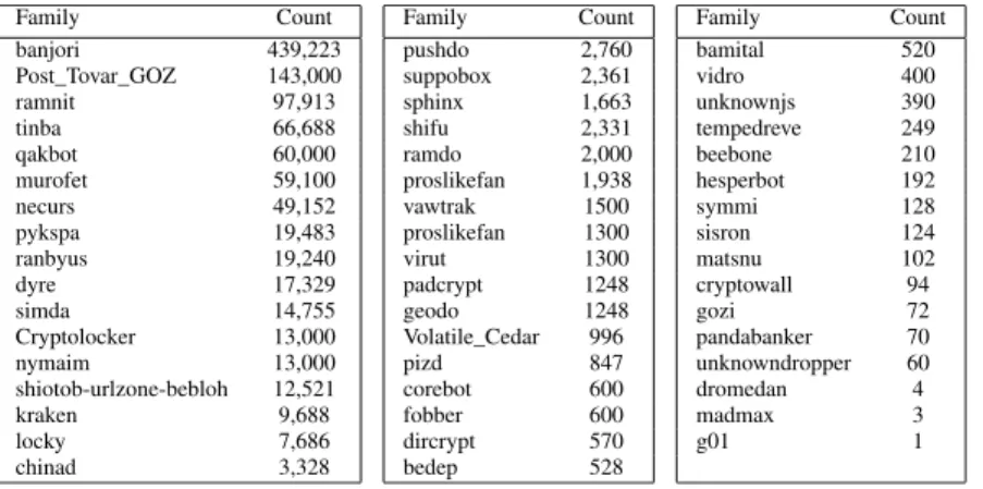
TABLE 3. Distribution of DGA families in the ground truth dataset.

(presumably) correct because they are obtained through reverse engineering malware, as explained in SectionIV-A. The downside is that obtaining such reliable labels is labor intensive, which explains why the ground truth dataset is fairly small (2M instances in total). In Section IV-B we explain how to overcome this problem by using heuristic labeling rules to obtain a large noise-not-free yet practi-cal dataset (approx. 50M instances) from real traffic data. In SectionVwe present and compare the results of classifiers trained on both kind of datasets, i.e. with ground truth as well as with weakly labeled real traffic data.

A. SMALL GROUND TRUTH DATASET

We collected a small ground truth dataset with 1 million DGA domain names obtained from the Bambenek Consulting feeds1 (positive examples), and the top 1 million domain names from Alexa2(negative examples). As is common when running experiments on datasets with hundreds of thousands of instances or more, we randomly split this data into 80% for training, 10% for validation, and 10% for testing, keeping the 50-50 ratio of positive vs. negative examples throughout.

Alexa ranks websites based on their popularity in terms of number of page views and number of unique visitors.

1_{http://osint.bambenekconsulting.com/feeds/, Accessed 2017-07-23} 2_{https://www.alexa.com/topsites, Accessed 2017-05-28}

It only retains the websites’ SLD, aggregating across any sub-domains. For example, according to Alexa, the five highest ranked domain names in terms of popularity on 2017-10-26

aregoogle.com,youtube.com,facebook.com baidu.com, and

wikipedia.org. For our experiments, we assume that the top 1 million domain names in this ranking are benign domain names, although it is possible that the bottom of the ranking may contain some noise.

In addition to these benign domain names, we collected 1 million DGA domain names from the Bambenek Consult-ing feeds for three different days, namely Jun 24, Jul 22, Jul 23, 2017. Table 3 shows the distribution of the 1M collected DGA domain names across 50 different known malware families. They were obtained by reverse engi-neering the known malware family, and generating lists of domain names with the reverse engineered malware with the random seeds for the specific days (see above). Note that our goal in this paper is the development of deep neural network classifiers that can detect DGAs without the need to reverse engineer malware families. An impor-tant advantage of such classifiers is that they can be used against new and previously unknown malware families. Besides the small ground truth labeled dataset described in this section, we therefore train our deep networks on a heuristically labeled real traffic dataset described next.

B. HEURISTICALLY LABELED REAL TRAFFIC DATA

The real traffic data originates from a real-time stream of passive DNS data. It consists of roughly 10-12 billion DNS queries per day collected from subscribers including ISPs (Internet Service Providers), schools, and businesses, from September 2015 through November 2017. As explained in SectionIandII, DGA domains are generated dynamically. The structure of these domain names is typically based on a time-dependent random seed, such as the current date, weather forecasts, or the trending topics on Twitter.com at that moment. The botmaster registers only very few of the domain names generated by a DGA. As a result, almost all of the requests from infected botnets to resolve DGA domain names trigger an NXDomain response. In addition, DGA domains have a shorter and very distinguishing lifes-pan compared to legitimate domains. Legitimate domains occur and reoccur for a longer period of time than DGA domains do. A unique DGA domain is normally generated only once on the same infected system. Different infected systems will generate the same DGA domains (relying on the same time dependent seed that is publicly available to all infected systems) within a small time window so that a registered DGA domain can have a high hit rate to be cost effective. Leveraging the fact that DGAs leave a characteristic trace of unsuccessful lookups (NXDomains) and that the domain names that they generate are typically short-lived, we use the heuristic filtering rules below for automatically creating a large dataset of positive and negative examples that can subsequently be used to train deep neural networks. It is important to observe that the temporal information about the lifespan of the domain names is only used for the creation of the dataset. The classifiers proposed in Section III and evaluated in SectionVonly rely on the domain name string itself as input, and can be deployed to detect DGA domain names from the moment that they appear in DNS traffic, without any prior knowledge of what their lifespan will be. 1) HEURISTIC LABELING RULES

We take as negative examples (potentially legitimate domains) those domain names which:

• have been resolved at least once

• never resulted in an NXDomain response, and

• span more than 30 days (span is defined as the number of days between the first and last query for a given domain) We take aspositive examples(potentially malicious domains) those which:

• never resolved

• consistently resulted in NXDomain at least 10 times, and • have all occurrences within the span of 7 days with

standard deviation 3 days or less

We apply these filtering rules to A and AAAA type DNS queries (a.k.a. IPv4 and IPv6 address records). We exclude samples with a second label of less than 10 characters, which serves to minimize noise [10].

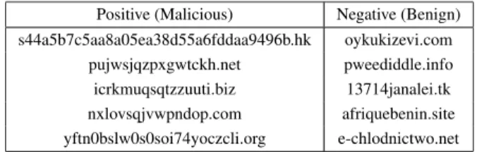
TABLE 4.Example domain names selected from real traffic. They are labeled as positive (first column) or negative (second column) according to our heuristic labeling rules.

Table 2 contains an overview of the training and test datasets created using the selected real traffic data. From the filtered domain names that were observed for the first time from September 2015 through August 2017, we selected roughly 40M instances and assigned them to a ‘‘Retro’’ dataset, split into 80% for training, 10% for validation (parameter tuning), and 10% for testing. In addition, filtered domains that were observed for the first time in the months September and October 2017 are reserved for testing pur-poses only; we refer to these sets as the prospective sets (see ProsSep-Test, ProsOct-Test) in Table2) in the sense that sam-ples in these sets are born after training time. The prospective data is used to evaluate the performance of the classifiers on future traffic, as it consists of domains observed from a later time period and not present in the training set. While the number of positive examples in these prospective sets is roughly equal, the number of negative examples appears to decline. This is simply a result of the time at which the data was collected (December 2017) and the filtering rules, in particular the requirement for a domain name to have an observed span of at least 30 days before it is considered a negative example. As time goes on, it becomes easier to satisfy the requirement. As a result, when re-collecting the prospective dataset for a particular month at a future time point, the number of negative examples tends to grow. To compensate this negative sample size reduction, we add negative samples that were observed for the first time from September 2015 through August 2017 and are not included in the Retro dataset into each of the prospective datasets because negative samples or legitimate domain names don’t change over the time.

Examples from the real traffic data are shown in Table4. Checking against a public repository of DGA domains, DGArchive [27], we confirm that the positives shown are real DGA domains. The negatives shown are not recorded as DGA domains on DGArchive.

V. RESULTS

In this section, we present the results of all architectures from SectionIIItrained separately with the ground truth data and with the real traffic data from SectionIVas well as with a combination of both kinds of data. Note that this gives rise to 15 deep neural network classifiers. Indeed, each architecture from SectionIIIresults in three kinds of classifiers that have the same structure but differ in the data they are fed with

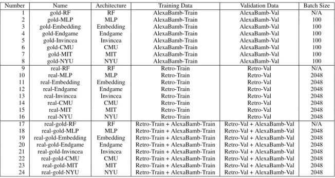
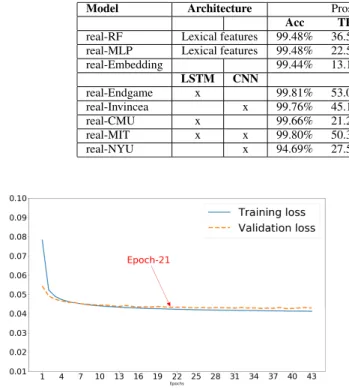
TABLE 5. Overview of trained models, with a specification of the data that was used for training and validation (hyperparameter tuning).

for training: the first kind of classifier is trained on ground truth data, the second one is trained on weakly labeled real traffic data, and the third one on a combination of both. This allows us to compare the performance of classifiers trained on supervised high quality training data versus on noisy, but high-volume data obtained by our heuristic labeling method. For comparison purposes, for each kind of training dataset, we have also trained a Random Forest (RF) and a Mul-tilayer Perceptron (MLP) on the following 11 features, extracted from each domain name string (see [1], [28]): ent (normalized entropy of characters); nl2 (median of 2-gram); nl3 (median of 3-gram); naz (symbol character ratio); hex (hex character ratio); vwl (vowel character ratio); len (domain label length); gni (gini index of characters); cer (classification error of characters); tld (top level domain hash); dgt (first character digit). Tree ensembles, includ-ing RFs, are a frequently used, state-of-the-art method for DGA classification based on human defined lexical fea-tures [2], [4], [6], [9], [10]. Feature based approaches to DGA detection, including RFs, logistic regression, and sup-port vector machines (SVMs), are systematically resup-ported in the literature to be outperformed by featureless deep learning methods. The findings we report in this section are in line with this. Since for the RF and the MLP there is no need to fix the length of the domain names to 75 characters, we extracted the 11 features directly from the domain names, without the preprocessing described in SectionIII-A. The RF consists of 100 trees. The MLP has a single hidden layer with 128 nodes. The values of the 11 features are normalized so that they are all on the same scale before presenting them to the MLP.

An overview of all trained models is presented in Table5. The MLP and all deep learning models were trained using

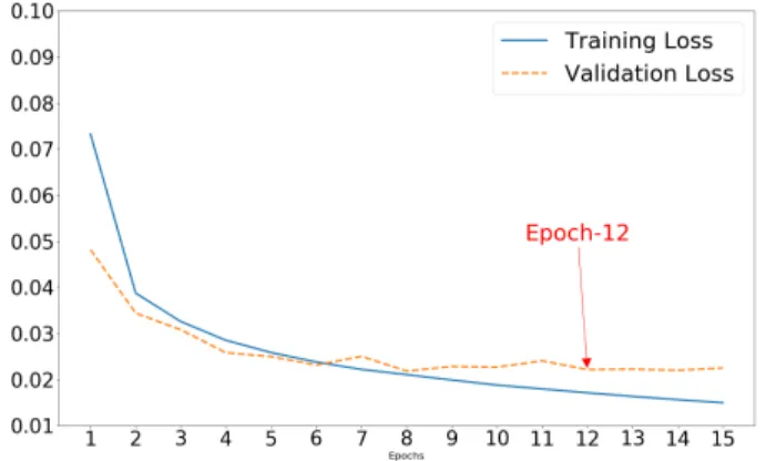
FIGURE 1. Training and validation loss curves for gold-endgame model.

Keras [29] while the RF was trained using sklearn [30], using the default settings for parameters unless specified otherwise. All deep learning models were trained with a learning rate of 0.001. Other details about the parameter settings for the deep learning models can be found in the Keras code snippets provided by Yuet al.[9].

A. TRAINING AND TESTING ON GROUND TRUTH DATA

Figure1–6 show the training and validation loss curves for models 3-8 from Table5, i.e. the deep learning models trained on the small ground truth dataset. In each figure there are one or more epochs where the validation curve increases, which indicates that we trained the models sufficiently long, and that further training would result in overfitting. Among all epochs, we then selected the epoch that gave the highest true positive rate (TPR) at a false positive rate (FPR) of 0.001 on the validation data. The displayed epochs indicate where we stopped the training to obtain the models used to produce the

FIGURE 2. Training and validation loss curves for gold-CMU model.

FIGURE 3. Training and validation loss curves for gold-NYU model.

FIGURE 4. Training and validation loss curves for gold-invincea model. final results in Table 6 and10. The training loss is higher than the validation loss in the pictures in Figure 1–6because the loss against the training data is computed in an average way across batches (the batch size is 100) while dropout is being applied, whereas performance on the validation set is determined at the end of each epoch with dropout disabled.

The accuracy of each of the trained models when applied to the ground truth test data AlexaBamb-Test is recorded in Table6. In addition to accuracy, this table includes the true positive rate (TPR) and false positive rate (FPR) for each of the models. Recall that TPR =TP/(TP +FN) and FPR= FP/(FP +TN) where TP, FP, TN, and FN are the number of true positives, false positives, true negatives, and false

FIGURE 5. Training and validation loss curves for gold-MIT model.

FIGURE 6. Training and validation loss curves for gold-embedding only model (baseline model).

negatives respectively. A low false positive rate is very impor-tant in deployed DGA detection systems, because block-ing legitimate traffic is highly undesirable. All classifiers in Table6output a probability that a given instance belongs to the positive class, so we can tune a threshold probability at which to consider a prediction positive. For each model, we choose this threshold such that the model trained over the training data has a 0.001 FPR over the validation data. Then we report the accuracy, TPR and FPR obtained with this classification threshold over the test data.

Finally, we also report AUC@1%FPR, which is the inte-gral of the ROC curve from FPR=0 to FPR=0.01 on the test data. Note that the highest absolute AUC@1%FPR value that can theoretically be obtained is 0.01, in other words, the absolute value of AUC@1%FPR ranges between 0 and 0.01. In Table6we denote the AUC@1%FPR achieved by the classifiers as a percentage of the ideal score. The gold-CMU model for instance, which is the best performing model, achieves an AUC@1%FPR of 98.25%, corresponding to an absolute AUC@1%FPR score of 0.009825.

As expected, the FPR of all classifiers in Table6is around 0.001: we tuned a classification threshold for the classifiers that produces a FPR of 0.001 on the validation data, and it is reassuring to see the same FPR emerge for the classifiers on the test data. There is a clear variation in the TPR that the classifiers achieve against that small FPR. While the Random

TABLE 6. Results for classifiers trained with ground truth alexabamb-train when applied to ground truth test data alexabamb-test. Accuracy, TPR, FPR are w.r.t. a threshold that gives a FPR of 0.001 on alexabamb-val.

TABLE 7. Examples of domain names from ground truth test data alexaBamb-test that were either misclassified by the random forest or by the deep neural networks trained on alexabamb-train. For the malicious domain names, the name of the malware family is shown between parentheses.

Forest is only able to ‘‘catch’’ 83% of the malicious domain names, all the deep neural network architectures achieve a recall of 97-98%. The baseline neural network consisting of only an embedding layer as its hidden layer clearly performs the worst with a TPR of less than 69%, highlighting that it is advantageous to extend the network architecture with one or more LSTM or CNN layers. Interestingly, there is little to no variation among the five deep neural network architectures in terms of TPR.

Table 7 contains examples of domain names from the ground truth test data that were randomly selected among those misclassified by either the Random Forest or by all five deep neural networks. Inspecting the column of the benign domain names, i.e. the Alexa domain names, it is interesting to note that most of those misclassified by the ground truth trained deep neural networks (bottom left in the table) come across as gibberish that a human annotator would likely also classify as malicious. As also evident from the top right of Table7, the deep neural networks have become very good at considering such gibberish-looking domain names to be malicious, even though they were never explicitly told to do so (unlike the Random Forest, which explicitly includes a normalized entropy of characters feature). The fact that the malicious domain names at the bottom right of Table7were missed by the deep neural networks might be due to our delib-erate choice to tune the classification threshold to achieve a very low FPR. This makes all the classifiers hold back from labeling a domain name as malicious if they are not almost completely certain. As explained above, a low FPR is very important in deployed DGA detection systems, as blocking legitimate traffic is highly undesirable. Note that if a deployed

DGA detection system would rely on the Random Forest classifier, it would block all domain names from the first row in Table7, whereas, if it would rely on any of the deep neural network classifiers, it would block all domain names from the second row in Table7. The domain names from the first column would have been unjustly blocked. For those negatively affected by this, it would be easier to ‘‘understand’’ (and perhaps forgive) the decisions made by the deep neural network classifiers, as they are more in line with decisions that a human would make when confronted with these domain name strings.

As Table8shows there is a substantial distinction among the different models in terms of complexity (number of parameters that have to be learned during the training process) and required training time per epoch. The platform used for training is an AWS virtual machine with access to multiple GPUs. Both the number of epochs needed to train a network, and the number of seconds required per epoch, are contribut-ing factors to the overall traincontribut-ing runtime. The NYU model took less than 8 minutes to train, while the CMU model took as much as 10 hours. The last column in Table8 shows the time needed to classify 200K domain names with an already trained model. The ranking of the deep networks in terms of this ‘‘scoring time’’ coincides with the ranking in terms of training time. Given that all deep networks achieve a similar accuracy (TPR), the NYU model with it short training and scoring time comes out as the winner.

B. TRAINING AND TESTING ON REAL TRAFFIC DATA

Our weakly labeled real traffic data set is an order of magni-tude larger than our ground truth data (50M vs. 2M). Training

TABLE 8. Comparison of complexity and efficiency of classifiers for DGA detection trained on ground truth data alexaBamb-train. The complexity refers to the number of parameters that have to be learned in the deep learning architectures. The training time is reported in terms of seconds needed for an epoch times the number of epochs. The scoring time is the time in seconds needed to label 200K domain names by an already trained model.

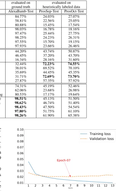
TABLE 9. Results for classifiers trained with real traffic data retro-train when applied to the prospective datasets obtained from real traffic. For the RF models, accuracy and TPR are w.r.t. a threshold that gives a FPR of 0.0002 on retro-val. For all other models, accuracy and TPR are w.r.t. a threshold that gives a FPR of 0.0001 on retro-val.

FIGURE 7. Training and validation loss curves for the real-endgame model, i.e. the model that is trained on retro-train, using retro-val as validation data.

on the real traffic data and keeping the batch size fixed at 100 results in more than 25 times as many weight updates per epoch, causing the optimization algorithm to try to learn too fast, giving rise to decreasing accuracy convergence curves. Rather than altering the learning rate, we solved this learn-ing problem by increaslearn-ing the batch size to 2048, which – as a welcome side-effect – also decreased the runtime significantly.

We trained all ‘‘real’’ models, i.e. models 9-16 from Table5, on the Retro-Train dataset from Table2, and used the Retro-Val validation dataset from Table 2 for hyperpa-rameter tuning, such as determining the number of epochs at which to stop training the neural networks, and selecting a classification threshold to achieve a desired FPR. The ‘‘real’’ models were trained on a workstation with an NVIDIA Titan

Xp GPU and 12 GB RAM. Figure7depicts, as an example, the train and validation loss curves for the real-Endgame model. Compared to Figure1, training on the weakly labeled dataset took approx. twice as many epochs as training on the ground truth dataset.

Table 9 contains the results for the classifiers that are trained on the weakly labeled real traffic data only, and evaluated on the prospective datasets with the same kind of heuristically labeled real traffic data. Keep in mind that in the heuristically labeled data, a domain name is labeled as positive (suspicious) if it was queried at least 10 times, never resolved, and all queries were within a time span of 7 days. Similarly, a domain name is labeled as negative (non-suspicious) if it was queried during a time span of at least 30 days and always resolved. When evaluating classi-fiers on the prospective real traffic datasets, we are effectively evaluating their ability to predict, based solemnly on a domain name string, whether that domain is a long-living, resolving domain (negative example) or whether it is a short-living domain that will never resolve (positive example).

The accuracy and TPR values reported in Table9for all models other than the RFs are with respect to a classifi-cation threshold that gives a FPR of 0.0001 on Retro-Val. We measured the achieved FPR obtained with this classifica-tion threshold on the prospective datasets as well. We found it to be 0.000099 consistently and decided to omit it from the table. The accuracy scores are very high, which is not very surprising given that the prospective datasets are imbalanced, i.e. they contain many more negative than positive examples. The more interesting metrics to inspect are therefore the TPR

TABLE 10. Predictive performance overview of all trained models, compared in terms of AUC@1% on alexabamb-test dataset and [email protected]% across different prospective test datasets.

and the [email protected]%. The latter is the integral of the ROC curve from FPR=0 to FPR=0.001 on the prospective data. As in Table6, it is reported as a percentage of the ideal value. For example, the real-MIT model achieves an [email protected]% of 72.69% on the prospective data from Sep 2017, which corresponds to an absolute [email protected]% value of 0.0007269 (the maximum possible being 0.001).

The first obvious observation is that the results in Table9

are significantly lower than those in Table 6, which comes as no surprise given the quality of the labels in the data. Indeed, the real traffic data is likely to contain a lot of noise because of the heuristic labeling rules. A second noteworthy observation is that there is a substantial amount of variation in the AUC scores of the five deep neural network models in Table9, ranging for instance from 44.45% (the real-CMU model) to 72.69% (the real-MIT model) on the prospective data from Sep 2017. This is unexpected and very unlike the evaluation on the ground truth dataset in Table 6, for which the AUC scores of all ground truth trained deep neural networks differed by less than 1%. The best performing models on heuristically labeled data are the real-Endgame (LSTM) and the real-MIT (CNN +LSTM) models. They both achieve [email protected]% scores that are above 72% when evaluated against future (prospective) weakly labeled data, which means that they can predict surprisingly accurately when a new domain name will never resolve and live only shortly. This confirms that there is a clear distinguishing signal in the domain name strings that are labeled as positive vs. negative by our heuristic labeling rules, even though the labeling rules themselves do not use any information derived from the domain name string at all.

FIGURE 8. Training and validation loss curves for the real-gold-endgame model, i.e. the real-endgame model trained further on alexabamb-train, using alexabamb-val as validation data.

C. CROSS-DATASET RESULTS

Table10 contains results for classifiers that are trained on weakly labeled real traffic data and cleanly labeled ground truth data combined, the so-called ‘‘real-gold’’ models from Table5. For all neural network based models, we have taken advantage of the fact that neural networks are very suitable for online learning, meaning that it is possible to first train them with real traffic data (Retro-Train) and then further update the weights by continuing the training with ground truth exam-ples (AlexaBamb-Train). Train and validation loss curves for the real-gold-Endgame model are depicted in Figure8

as an example. In the case of Random Forests, where such pretraining is not possible, we simply combine all data (Retro-Train+AlexaBamb-Train) and present it all to the RF learning algorithm at once.

TABLE 11. Examples of malicious domain names that were caught by the real-gold-invincea model and not by the gold-invincea model.

All models are evaluated on the ground truth data (Alexa-Bamb-Test, in terms of AUC@1%) and on the prospective datasets (in terms of [email protected]%). For comparison purposes, for the ‘‘gold’’ and ‘‘real’’ models, some results from Table6

and Table 9 are recalled. Furthermore, they are completed with cross-dataset results, such as the results for the classi-fiers trained on the real traffic data when evaluated on the ground truth data test set (Alexa-Bamb-Test). As mentioned in SectionIV, the filtered real traffic data does not contain domain names with a second label that is shorter than 10 char-acters, which implies that the ‘‘real’’ models have never seen such domain names during training. For this reason, when evaluating these ‘‘real’’ models on the ground truth data test set, we systematically classify all domains that are shorter than 10 characters as negative (benign) and use the trained classifier to infer a class label for all other domains.

The results in Table10reveal that models trained on ground truth data (the ‘‘gold’’ models) do not perform well against the prospective real traffic data, while models trained on weakly labeled real traffic data (the ‘‘real’’ models) do not perform well against ground truth data. Classifiers pre-trained on the heuristically labeled data and post-trained on ground truth data (the ‘‘real-gold’’ models) perform reasonably well against heuristically labeled data, and, as shown in the bottom left of Table 10, they perform really well against ground truth data. Given that the AUC@1% scores of the ‘‘gold’’ models are already very high to begin with, leaving only little room for improvement, the improved AUC@1% scores of the ‘‘real-gold’’ models are noteworthy.

It is interesting to observe that the gold-Invincea model, which was the weakest among the ground truth trained deep neural network models when applied to the AlexaBamb-Test set (97.47%), became the strongest model of all (i.e. the real-gold-Invincea model) after pretraining on the heuristically labeled real traffic data (98.62%). As we know from Table8, this is the most complex model, i.e. with the largest number of parameters, and it can thrive when given enough data. Table11contains examples of malicious domain names that were correctly detected as such by the Invincea model when trained on a combination of weakly labeled real traffic data and cleanly labeled ground truth data. The Invincea model that was trained on ground truth data alone overlooked these malicious domain names, illustrating the fact that there is

TABLE 12.AUC@1% results for all trained deep neural network models when evaluated on different ground truth datasets.

practical value in pretraining the deep neural network clas-sifiers with weakly labeled real traffic data.

To verify that the improvement obtained with pretrain-ing on heuristically labeled real traffic data is statistically significant, we evaluated the trained models on additional test data, with malicious domain names that appeared in traffic after the data that was used for training. Recall that all data used for training the models in Table10was collected between 2015-2017. In Table 12 we tested these models on datasets AlexaBambJun29-Test, AlexaBambJul01-Test, and AlexaBambJul03-Test. Each of these datasets contains 100K malicious domain names from the Bambenek feeds for June 29, 2018, July 01, 2018, and July 03, 2018 respectively, as well as the 100K Alexa domain names from AlexaBamb-Test. The first column with results in Table 12 contains the AUC@1% score for the various deep neural network models when trained on ground truth data only, and the sec-ond column contains the results when the ground truth data is augmented with real traffic data during training. Using the Wilcoxon test we determined that the improvement observ-able in Tobserv-able12is statistically significant at the 1% signif-icance level with a p-value of 6.104E-5. This should come as no surprise, as a strict improvement was observed for each experiment, highlighting that the use of real traffic data consistently makes the classifiers significantly more accurate.

VI. CONCLUSION

In this paper we have investigated the use of deep neural network based classifiers for DGA detection, trained with large amounts of weakly labeled data obtained from real traffic. The heuristic labeling rules that we proposed to obtain a noise-not-free yet practical training dataset do not make any assumptions about the structure of the domain name strings themselves, nor the algorithms that were used to generate them. Instead, they leverage the fact that DGAs leave a characteristic trace of NXDomain responses, and that DGA domain names have a typical, short lifespan. We have shown that enriching ground truth data trained DGA classi-fiers with automatically collected and filtered weakly labeled real traffic data improves their predictive accuracy, resulting

in classifiers that achieve very high AUC scores (98% and above).

The trained classifiers themselves only require the domain name string as input, which means that they can be deployed to detect DGA domain names in real-time as part of a resolver, on a per domain basis, without requiring knowledge about the expected lifespan of the domain name or any other potentially privacy sensitive information such as the IP address of the host requesting the domain name. Infoblox has created an architecture to include the DGA detection classifier that is served by Google’s TensorFlow Serving [31] into its DNS services. A DNS query is sent to the resolver and the clas-sifier in parallel. When the domain name is resolved and the classification result is positive, the resolved IP address is suspected to be intended for C&C communication, and blocked accordingly. In the product, the false positive rate is set to be as low as 0.001%. Since a C&C server’s IP address will be reused over time by a number of malicious domains, any lowered true positive rate for detecting DGA domains resulting from the lower false positive rate setting does not significantly reduce the rate of capturing C&C IP addresses.

REFERENCES

[1] B. Yu, L. Smith, and M. Threefoot, ‘‘Semi-supervised time series modeling for real-time flux domain detection on passive DNS traffic,’’ inProc. MLDM, Stain Petersburg, Russia, 2014, pp. 258–271.

[2] M. Antonakakiset al., ‘‘From throw-away traffic to bots: Detecting the rise of DGA-based malware,’’ presented at the USENIX Secur. Symp., Bellevue, WA, USA, 2012. [Online]. Available: https://www.usenix. org/system/files/conference/usenixsecurity12/sec12-final127.pdf [3] S. Schiavoni, F. Maggi, L. Cavallaro, and S. Zanero, ‘‘Phoenix:

DGA-based botnet tracking and intelligence,’’ inProc. DIMVA, Egham, U.K., 2014, pp. 192–211.

[4] S. Schüppen, D. Teubert, P. Herrmann, and U. Meyer, ‘‘FANCI: Feature-based automated NXDomain classification and intelligence,’’ presented at the USENIX Secur. Symp., Baltimore, MD, USA, 2018. [Online]. Available: https://www.usenix.org/system/files/conference/ usenixsecurity18/sec18-schuppen.pdf

[5] P. Lison and V. Mavroeidis. (2017). ‘‘Automatic detection of malware-generated domains with recurrent neural models.’’ [Online]. Available: https://arxiv.org/pdf/1709.07102.pdf

[6] J. Woodbridge, H. S. Anderson, A. Ahuja, and D. Grant. (2016). ‘‘Pre-dicting domain generation algorithms with long short-term memory net-works.’’ [Online]. Available: https://arxiv.org/pdf/1611.00791.pdf [7] J. Saxe and K. Berlin. (2017). ‘‘eXpose: A character-level

convolu-tional neural network with embeddings for detecting malicious URLs, file paths and registry keys.’’ [Online]. Available: https://arxiv.org/pdf/ 1702.08568.pdf

[8] D. Tran, H. Mac, V. Tong, H. A. Tran, and L. G. Nguyen, ‘‘A LSTM based framework for handling multiclass imbalance in DGA botnet detection,’’

Neurocomputing, vol. 275, pp. 2401–2413, Jan. 2018.

[9] B. Yu, J. Pan, J. Hu, A. Nascimento, and M. De Cock, ‘‘Character level based detection of DGA domain names,’’ inProc. WCCI, Rio de Janeiro, Brazil, 2018, pp. 4168–4175.

[10] B. Yu, D. Gray, J. Pan, M. De Cock, and A. Nascimento, ‘‘Inline DGA detection with deep networks,’’ inProc. ICDMW, New Orleans, LA, USA, Nov. 2017, pp. 683–692.

[11] B. Dhingra, Z. Zhou, D. Fitzpatrick, M. Muehl, and W. Cohen, ‘‘Tweet2Vec: Character-based distributed representations for social media,’’ inProc. ACL, vol. 2, Berlin, Germany, 2016, pp. 269–274. [12] S. Vosoughi, P. Vijayaraghavan, and D. Roy, ‘‘Tweet2vec: Learning tweet

embeddings using character-level CNN-LSTM encoder-decoder,’’ inProc. SIGIR, Pisa, Italy, 2016, pp. 1041–1044.

[13] X. Zhang, J. Zhao, and Y. LeCun, ‘‘Character-level convolutional networks for text classification,’’ inProc. Adv. Neural Inf. Process. Syst., vol. 28, 2015, pp. 649–657.

[14] D. Plohmann, K. Yakdan, M. Klatt, J. Bader, and E. Gerhards-Padilla, ‘‘A comprehensive measurement study of domain generat-ing malware,’’ presented at the USENIX Secur. Symp., Austin, TX, USA, 2016. [Online]. Available: https://www.usenix.org/system/files/ conference/usenixsecurity16/sec16_paper_plohmann.pdf

[15] J. Kwon, J. Lee, H. Lee, and A. Perrig, ‘‘PsyBoG: A scalable botnet detection method for large-scale DNS traffic,’’Comput. Netw., vol. 97, pp. 48–73, Mar. 2016.

[16] J. Abbink and C. Doerr, ‘‘Popularity-based detection of domain generation algorithms,’’ inProc. ARES, Reggio Calabria, Italy, 2017, pp. 1–79. [17] R. R. Curtin, A. B. Gardner, S. Grzonkowski, A. Kleymenov, and

A. Mosquera. (2018). ‘‘Detecting DGA domains with recurrent neural networks and side information.’’ [Online]. Available: https://arxiv.org/pdf/ 1810.02023.pdf

[18] I. Goodfellowet al., ‘‘Generative adversarial nets,’’ presented at the NIPS, Montréal, QC, Canada, 2014. [Online]. Available: http://papers.nips.cc/ paper/5423-generative-adversarial-nets.pdf

[19] I. Goodfellow, J. Shlens, and C. Szegedy. (2014). ‘‘Explaining and har-nessing adversarial examples.’’ [Online]. Available: https://arxiv.org/pdf/ 1412.6572.pdf

[20] H. S. Anderson, J. Woodbridge, and B. Filar, ‘‘DeepDGA: Adversarially-tuned domain generation and detection,’’ inProc. AISec, Vienna, Austria, 2016, pp. 13–21.

[21] S. Yadav, A. K. K. Reddy, A. Reddy, and S. Ranjan, ‘‘Detecting algorith-mically generated malicious domain names,’’ inProc. IMC, Melbourne, VIC, Australia, 2010, pp. 48–61.

[22] S. Yadav, A. K. K. Reddy, A. L. N. Reddy, and S. Ranjan, ‘‘Detecting algorithmically generated domain-flux attacks with DNS traffic analysis,’’

IEEE/ACM Trans. Netw., vol. 20, no. 5, pp. 1663–1677, Oct. 2012. [23] S. Hochreiter and J. Schmidhuber, ‘‘Long short-term memory,’’Neural

Comput., vol. 9, no. 8, pp. 1735–1780, 1997.

[24] D. Kingma and J. Ba. (2014). ‘‘Adam: A method for stochastic optimiza-tion.’’ [Online]. Available: https://arxiv.org/pdf/1412.6980.pdf

[25] N. Srivastava, G. Hinton, A. Krizhevsky, I. Sutskever, and R. Salakhutdinov, ‘‘Dropout: A simple way to prevent neural networks from overfitting,’’J. Mach. Learn. Res., vol. 15, no. 1, pp. 1929–1958, 2014.

[26] W. Linget al.(2016). ‘‘Finding function in form: Compositional character models for open vocabulary word representation.’’ [Online]. Available: https://arxiv.org/pdf/1508.02096.pdf

[27] DGArchive Fraunhofer FKIE. Accessed: May 28, 2017. [Online]. Avail-able: https://dgarchive.caad.fkie.fraunhofer.de/

[28] B. Yu, L. Smith, M. Threefoot, and F. Olumofin, ‘‘Behavior analysis based DNS tunneling detection and classification with big data technologies,’’ in

Proc. IoTBD, Rome, Italy, 2016, pp. 284–290.

[29] F. Cholletet al.(2015).Keras. [Online]. Available: https://keras.io [30] F. Pedregosaet al., ‘‘Scikit-learn: Machine learning in Python,’’J. Mach.

Learn. Res., vol. 12, pp. 2825–2830, Oct. 2011.

[31] Google. Accessed: Jun. 26, 2018. [Online]. Available: https://www. tensorflow.org/serving/

BIN YUreceived the Ph.D. degree in electronic engineering from Tsinghua University, China. He is a Chief Data Scientist at Infoblox, Santa Clara, CA, USA, where he pioneered big data analyt-ics to detect malicious DNS traffic, using deep learning and artificial intelligence techniques to keep pace with fast changing malware evolution. He worked with many high tech companies in Silicon Valley at senior leadership positions and led projects of machine learning and artificial intelligence for internet search, medical imaging, computer vision, and e-commerce. He has a rich experience in both academia and industry for more than 25 years. He was a Postdoctoral Fellow with the Pattern Recog-nition and Image Processing Lab, Michigan State University, USA, and as an Associate Professor with Beijing Jiaotong University, China. He has published more than 50 peer reviewed papers and holds patents in artificial intelligence, deep learning, machine learning, image processing, and cyber-security. He is a Senior Member of the IEEE Computer Society.

JIE PANreceived the B.S. degree in management information systems from The Ohio State Uni-versity, USA, in 2013, and the M.S. degree in computer science and systems from the University of Washington, USA, in 2017. During his gradu-ate studies, he was a Student Assistant research-ing the detection and classification of malicious domain names with machine learning techniques. He is currently with Amazon Video, Seattle, USA, where he uses machine learning techniques to offer recommendations for consumers.

DANIEL GRAYreceived the B.S. degree in com-puter engineering and the M.S. degree in comcom-puter science and systems from the University of Wash-ington, USA, in 2016 and 2018, respectively. His M.S. research was on the use of deep learning to train classifiers for the detection of algorithmically generated domain names. He is currently a Soft-ware Engineer with Infoblox, Tacoma, USA.

JIAMING HUreceived the B.S. degree in com-puter science and technology from Zhejiang Wanli University, China, in 2005, and the M.S. degree in computer science and systems from the University of Washington, USA, in 2018. His M.S. research was on the use of deep learning to train classi-fiers for the detection of algorithmically generated domain. He is currently a Senior Deep Learning Scientist with Mythic, Inc., Palo Alto, USA. His current research interests include object detection, super resolution, low light image enhancement in computer vision, and AI auto-training infrastructure.

CHHAYA CHOUDHARYreceived the B.S. degree in computer science from Banasthali University, India, in 2011, and the M.S. degree in computer science and systems from the University of Wash-ington, USA, in 2019. Her master’s thesis was on the evaluation of state-of-the-art DGA classifiers against adversarial examples using autoencoders and generative adversarial networks. She is cur-rently a Data Scientist with Infoblox, where she is solving challenging data problems involving mal-ware detection and classification using machine learning and deep learning techniques.

ANDERSON C. A. NASCIMENTOreceived the B.S. degree in electrical engineering from the Uni-versity of Brasilia, Brazil, in 1998, and the M.S. and Ph.D. degrees in information and communi-cation engineering from The University of Tokyo, Japan, in 2001 and 2004, respectively. He was a permanent member of the Nippon Telegraph and Telecom Cryptography Research Group, Japan, and a Faculty Member with the University of Brasilia, Brazil. He is currently an endowed Asso-ciate Professor of information security and information technology with the School of Engineering and Technology, University of Washington, Tacoma, USA. His research interests include cryptography, information security, privacy, and machine learning applications.

MARTINE DE COCKreceived the M.S. and Ph.D. degrees in computer science from Ghent Univer-sity, Belgium, in 1998 and 2002, respectively. Her previous work experiences include positions as a Research Assistant and a Postdoctoral Fellow supported by the Fund for Scientific Research— Flanders, a Visiting Scholar with the BISC Group, University of California at Berkeley, Berkeley, USA, a Visiting Scholar with the Knowledge Sys-tems Laboratory, Stanford University, USA, and an Associate Professor with the Department of Applied Mathematics, Com-puter Science and Statistics, Ghent University. She is currently a Profes-sor with the School of Engineering and Technology, University of Wash-ington, Tacoma, USA, and a Guest Professor with Ghent University. She Co-Organized the KDDCup2013. She has more than 150 peer reviewed publications in international journals and conferences on artificial ligence, data mining, machine learning, information retrieval, web intel-ligence, and logic programming. Her current research interests include privacy-preserving machine learning, cybersecurity, and data analytics to improve the quality of healthcare. She is a Program Committee Member of numerous international conferences. She has served as an Associate Editor for the IEEE TRANSACTIONS ONFUZZYSYSTEMS.