Building Efficient Large-Scale Big Data Processing Platforms

(1)

University of Massachusetts Boston

ScholarWorks at UMass Boston

Graduate Doctoral Dissertations Doctoral Dissertations and Masters Theses

5-31-2017

Building Efficient Large-Scale Big Data Processing

Platforms

Jiayin Wang

University of Massachusetts Boston

Follow this and additional works at:https://scholarworks.umb.edu/doctoral_dissertations Part of theComputer Sciences Commons

This Open Access Dissertation is brought to you for free and open access by the Doctoral Dissertations and Masters Theses at ScholarWorks at UMass Boston. It has been accepted for inclusion in Graduate Doctoral Dissertations by an authorized administrator of ScholarWorks at UMass Boston. For more information, please [email protected].

Recommended Citation

Wang, Jiayin, "Building Efficient Large-Scale Big Data Processing Platforms" (2017).Graduate Doctoral Dissertations. 348.

(2)

BUILDING EFFICIENT LARGE-SCALE BIG DATA PROCESSING

PLATFORMS

A Dissertation Presented by

JIAYIN WANG

Submitted to the Office of Graduate Studies, University of Massachusetts Boston,

in partial fulfillment of the requirements for the degree of DOCTOR OF PHILOSOPHY

May 2017

(3)

(4)

BUILDING EFFICIENT LARGE-SCALE BIG DATA PROCESSING

PLATFORMS

A Dissertation Presented by

JIAYIN WANG

Approved as to style and content by:

Bo Sheng, Associate Professor Chairperson of Committee

Wei Ding, Associate Professor Member

Dan Simovici, Professor Member

Honggang Zhang, Associate Professor Member

Dan Simovici, Program Director Computer Science Program

Peter Fejer, Chairperson Computer Science Department

(5)

ABSTRACT

BUILDING EFFICIENT LARGE-SCALE BIG DATA PROCESSING

PLATFORMS

MAY 2017

JIAYIN WANG

B.S., XIDIAN UNIVERSITY, XI’AN, CHINA M.S., UNIVERSITY OF MASSACHUSETTS BOSTON Ph.D., UNIVERSITY OF MASSACHUSETTS BOSTON

Directed by: Professor Bo Sheng, Associate Professor

In the era of big data, many cluster platforms and resource management schemes are created to satisfy the increasing demands on processing a large volume of data. A general setting of big data processing jobs consists of multiple stages, and each stage represents a generally defined data operation such as filtering and sorting. To parallelize the job execution in a cluster, each stage includes a number of identical tasks that can be concurrently launched at multiple servers. Practical clusters often involve hundreds or thousands of servers processing a large batch of jobs. Resource management, that manages cluster resource allocation and job execution, is extremely critical for the system performance.

Generally speaking, there are three main challenges in resource management of the new big data processing systems. First, while there are various pending tasks from different jobs and stages, it is difficult to determine which ones deserve the priority

(6)

to obtain the resources for execution, considering the tasks’ different characteristics such as resource demand and execution time. Second, there exists dependency among the tasks that can be concurrently running. For any two consecutive stages of a job, the output data of the former stage is the input data of the later one. The resource management has to comply with such dependency. The third challenge is the inconsistent performance of the cluster nodes. In practice, run-time performance of every server is varying. The resource management needs to dynamically adjust the resource allocation according to the performance change of each server.

The resource management in the existing platforms and prior work often rely on fixed user-specific configurations, and assumes consistent performance in each node. The performance, however, is not satisfactory under various workloads. This dissertation aims to explore new approaches to improving the efficiency of large-scale big data processing platforms. In particular, the run-time dynamic factors are carefully considered when the system allocates the resources. New algorithms are developed to collect run-time data and predict the characteristics of jobs and the cluster. We further develop resource management schemes that dynamically tune the resource allocation for each stage of every running job in the cluster. New findings and techniques in this dissertation will certainly provide valuable and inspiring insights to other similar problems in the research community.

(7)

ACKNOWLEDGMENTS

I would like to express my sincere gratitude to the following people. I would not have been able to complete my dissertation without the support of them.

Firstly, I would like to thank my advisor, Professor Bo Sheng, for his continuous guidance and encouragement throughout my Ph.D. life with his patience, motivation, enthusiasm, and immense knowledge. I thank him for introducing me to the wonders of scientific research. I could not have imagined having a better advisor and mentor for my Ph.D. study. Meanwhile, I would like to offer my special thanks my committee, Professor Dan Simovici, Professor Wei Ding, and Professor Honggang Zhang, for their great support and insightful feedback and comments.

In addition, I wish to acknowledge the help provided by my research collaborators: Professor Ningfang Mi, Doctor Yi Yao, Doctor Ying Mao and Zhengyu Yang. My thanks also go to my labmates Teng Wang and Son Nam Nguyen for working together, and for all the fun we have had in the last five years. Many thanks to my friends in the Computer Science department Ting Zhang, Dong Luo, Dawei Wang, Yahui Di, and Akram Bayat, for the friendship and support.

Finally, I would like to thank everyone in my family. I am grateful to my parents Genjian Wang and Xiaopei Guo, and also my cousin Doctor Lingyin Li (my eternal role model and cheerleader) for always supporting me and loving me. Especially, I wish to thank my husband Shaohua Jia and my son Chenrui Jia for standing by me through the tough times and bringing happiness into my life.

(8)

LIST OF FIGURES

Figure Page

1.1 Typical deployment of large-scale big data computing systems . . . 2

1.2 General mechanism of _FRESH. . . 6

1.3 General mechanism of OMO. . . 7

1.4 General mechanism of eSplash . . . 8

2.1 MapReduce data processing scheme. . . 11

2.2 Structure of Apache Hadoop. . . 12

2.3 Job execution in Hadoop YARN . . . 13

3.1 Static slot configuration. . . 18

3.2 Dynamic slot configuration. . . 18

3.3 Makespan of simple workloads under FRESH and Fair scheduler. . . 41

3.4 Fairness of of simple workloads under FRESH andFair scheduler. . . 42

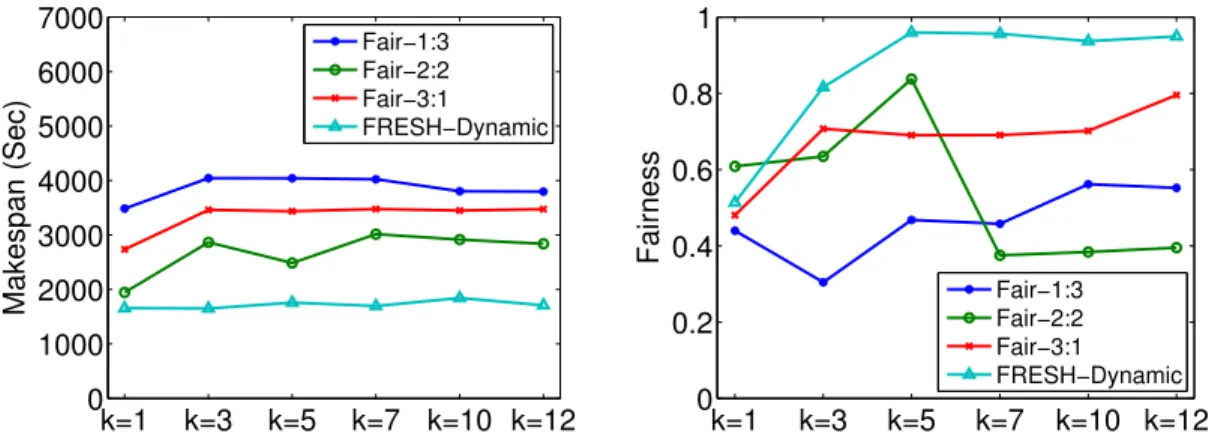
3.5 Makespan and fairness of set A with different values ofk . . . 43

3.6 Set A tasks execution and slots assignments with FRESH-dynamic(k= 5) . . . 43

3.7 Fairness of set A with different values ofk. . . 43

3.8 Makespan of set B∼E (with 10 slave nodes). . . 44

(12)

3.10 Makespan and fairness of set B with 20 slave nodes . . . 44

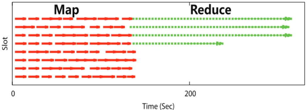
4.1 Slot allocation of one Terasort job with dynamic slot configuration (slowstart = 1). . . 52

4.2 Slot allocation of one Terasort job with dynamic slot configuration (slowstart = 0.6).. . . 52

4.3 Illustration of the proof. . . 55

4.4 Lazy Start of Reduce Tasks: illustrating the alignment of map phase and shuffling phase. . . 56

4.5 Map tasks are finished in 4 waves. . . 61

4.6 The tailing map task incurs an additional round . . . 61

4.7 Experiment with 3 jobs in a Hadoop cluster withFair scheduler: Solid lines represent map tasks and dashed lines represent reduce tasks. . . 62

4.8 System implementation . . . 66

4.9 Slot release prediction . . . 70

4.10 Last batch of map tasks . . . 71

4.11 Slot allocation in the execution of 8 Terasort jobs withFair scheduler and the default slowstart=0.05 . . . 72

4.12 Slot allocation in the execution of 8 Terasort jobs withFair scheduler and the default slowstart=1 . . . 73

4.13 Slot allocation in the execution of 8 Terasort jobs with FRESH and the default slowstart=1 . . . 73

4.14 Slot allocation in the execution of 8 Terasort jobs withOMOand the default slowstart=1 . . . 74

4.15 Execution time under Fair scheduler, FRESHand Lazy Start (with 20 slave nodes) . . . 76

4.16 Execution time under Fair scheduler, FRESHand Batch Finish (with 20 slave nodes) . . . 77

(13)

4.17 Execution time under _{Fair scheduler}, FRESH,Lazy Start, Batch

Finish and OMO (with 20 slave nodes) . . . 77

4.19 Execution time underOMO with: (a) different sizes of the input data and (b) different number of jobs. . . 79

4.18 Execution time in map + shuffling phase of simple workloads.. . . 82

5.1 Hadoop records the historic execution times of each type of tasks in each job for determining the candidate tasks for speculative execution . . . 86

5.2 An example of clustering 80 nodes: we collect the execution time of two types of tasks (the map tasks in WordCount and TeraSort), thus each P V is a two dimensional data. . . 92

5.4 System implementation . . . 97

5.5 Makespan without stragglers . . . 101

5.6 Increased makespan with a straggler on node level 1 . . . 102

5.7 Increased makespan with a straggler on node level 4 . . . 103

5.8 Increased makespan with a straggler which will be restarted . . . 104

5.3 The Speculative tasks created under bothLATE andeSplash: (1) without Straggler, (2) with one straggler on node level 1, (3) with one straggler on node level 4 . . . 107

(14)

LIST OF TABLES

Table Page

3.1 Set A: 12 mixed jobs . . . 34

3.2 Set D: 12 map-intensive mixed jobs . . . 35

3.3 Set E: 12 reduce-intensive mixed jobs . . . 35

3.4 Set B: 6 mixed jobs . . . 37

3.5 Set C: 24 mixed jobs . . . 37

4.1 Notations . . . 48

4.2 Execution times of 1 and 3 Terasort jobs with different slowstart values in traditional Hadoop systems. . . 52

4.3 Execution times of 1 and 3 Terasort jobs with different slowstart values and dynamic slot configuration. . . 53

4.4 Benchmark characteristics. . . 69

4.5 Sets of mixed jobs . . . 75

4.6 Execution time of Terasort benchmark under YARN and OMO (with 20 slave nodes).. . . 79

4.7 Makespan of set H with 40 slave nodes. . . 80

(15)

CHAPTER 1 INTRODUCTION

The past decades have witnessed a major change in data processing platforms, as the rapid growth of big data requires more and more applications to scale out to large clusters. From the statistics of IDC reports [1], there are 4.4 zettabytes (4.4 billion terabytes) of data exist in the digital universe and this number will be increased to 44 zettabytes by 2020. Besides structured data in database, unstructured data sets are generated in both academia and industry by various of modern technologies such as gene sequencers, wearable sensors, social networks (e.g., Facebook and Twitter), radio frequency ID (RFID), Internet of things (IoTs), and smartphones. Meanwhile, big data analytics is well used in almost everywhere of our daily life, such as healthcare, business, finance, traffic control, manufacturing, and retail. Powerful and efficient computer systems are required to process big data in a timely fashion. However, the traditional database system deployed in a single server is inadequate to deal with big data because of its increasing of volume, variety, velocity, and veracity. Therefore, many cluster-based scalable platforms have been developed to serve the growing demands for processing big data in parallel. Fig. 1.1 shows the family of approaches and mechanisms of emerging large-scale data processing systems. In a cluster, the input and output data are stored in a distributed file system such as HDFS (Hadoop Distributed File System). Upon the storage layer are deployed by different large-scale data computing systems such as MapReduce/Hadoop [2], Hadoop YARN [3], Mesos [4], Tez [5], and Spark [6]. A series of eco-systems are built upon

(16)

them to process multiple types of data and applications such as Hive [7], Pig [8], Shark [9], Storm [10], and Mahout [11].

Spark

HDFS

Hadoop Distributed File System

Hadoop YARN

Hadoop MapReduce

Mesos

Tez

Hive

Pig

Shark

Storm

Mahout

Figure 1.1: Typical deployment of large-scale big data computing systems

A general setting of big data jobs consists of a sequence of processing stages, and each stage represents a generally defined data operation such as filtering, merging, sorting, and mapping. To parallelize the job execution in a large-scale cluster, each stage includes a number of identical tasks that can be concurrently launched at multi-ple servers. This general setting of multi-stage data processing includes a wide range of data analysis products in practice. For example, MapReduce/Hadoop represents a typical two-stage process. Other representative applications with multi-stage data processing include chained MapReduce jobs for SQL-on-Hadoop queries, iterative ma-chine learning algorithms (e.g., pagerank, logistic regression, k-mean, and others in Mahout library), and scientific computation (e.g., data assimilation in GFS weather forecasting and hydrology, and partial differential equation based simulation).

In a large-scale cluster, resource management is extremely critical for the per-formance. It has been frequently reported that the resource utilization in big data

processing systems is unexpectedly low. For example, a production cluster with

thousands of servers at Twitter managed by Mesos has reported its aggregated CPU utilization lower than 20% even though 80% resource capacities of the cluster are reserved.

(17)

This dissertation aims to build efficient large-scale big data processing systems by exploring new resource management schemes to dynamically tune the resource allo-cation based on the characteristics of the data processing systems and job properties.

1.1 Research Challenges

In this section, we discuss the common characteristics of the current big data computing systems, and the main research challenges in resource management based on these characteristics. Our work is motivated by the following challenges.

1. Various workloads. Big data processing systems usually serve numerous kinds of applications submitted by various users concurrently. Every job consists of multiple stages and one unique operation is provided in each stage. Tasks from different stages of different jobs require dissimilar resource demands and yield varying execution time. For example, a typical MapReduce job contains two stages: map and reduce. The map stage focuses on disk I/O processing and the reduce stage is responsible for data analysis. Therefore, tasks in the map stage usually rely more on the disk I/O and the ones in the reduce stage require more resources on memory and CPU. Even in the reduce stage, different operations rely on different amounts of resources. For instance, in the text processing, sorting usually requests more memory resource than word counting. With different demands of resources, it is challenging to assign appropriate resources to numerous types of applications with multiple stages in order to give consideration to the execution times of all jobs and also fair resource sharing for each job.

2. Dependency of stages. Dependency usually exists between stages of every application in big data processing systems. For any two consecutive stages of a job, the output data of the former stage is the input data of the later one. On the one hand, the later stage cannot finish before its former stage. The resource management in the cluster needs to comply with such dependency. On the other hand, the later

(18)

one can start earlier before the completion of the former one. The first component in each stage (except the first stage in a job) is called shuffling. It is responsible for transferring the output data generated from the former stage to itself. Starting the shuffling phase earlier can help improve the performance by overlapping the shuffling phase and the finish of the previous stage. We find that this unique period plays an important role on the resource management. Appropriately determining the finish time of one stage and the start time of the next stage can avoid idle resources or accumulated data waiting for processing. However, different stages of various jobs generate varying sizes of data and the data transferring rate is changing all the time according to the system bandwidth and interference by the shuffling operations from other jobs. Therefore, it is challenging for the resource management to determine the best timing to start the later stages for different jobs.

3. Inconsistent performance of the cluster nodes. During the execution of any cluster in practice, the run-time performance of every node is varying. Many factors can impact the system performance of a server in the cluster, such as the number of processes the server is running at the same time, the memory occupation percent-age, and the competition of reading/writing operations to the disk. It requires the scheduler to adjust the resource allocation in real time according to the performance change of each server.

4. Node failures in the cluster. In a large-scale cluster, node failures and strag-glers (slow servers) are normality in practical. Fault tolerance is usually executed in the computing systems to handle this kind of issues. Speculation mechanism is a common solution to mitigate the impact of such failures. Basically, when a straggler is detected, a copy of its tasks (speculative tasks) will be created and assigned to another server to finish faster so that a job would not be as slow as the misbehaving tasks. Three requests should be taken into consideration for an effective and effi-cient speculative mechanism. First, it should be able to accurately identify stragglers

(19)

from normal slow nodes when every node in the cluster has different performance (i.e., a speculation mechanism should work well in a heterogeneous cluster). Second, when a node becomes abnormally slow, the speculation mechanism should detect this straggler rapidly. Finally, once a straggler is identified, its duplicated tasks should be assigned to appropriate nodes with good performance, since assigning duplicated tasks back to the stragglers or even slower nodes cannot improve the system performance or reduce the job execution time. However, we find that the existing speculative mechanisms cannot satisfy these three demands. In chapter 5, we will introduce our efficient speculative mechanism.

Above all, these characteristics provides both challenges and opportunities for the resource management schemes for the large-scale big data processing system. However, the existing ones have not thoroughly addressed these issues. In the disser-tation, we will introduce our new scheduling and resource management approaches to improving the efficiency, e.g., reducing the execution times of a batch of jobs (i.e., makespan) and increasing the system resource utilization, in the large-scale cluster computing systems.

1.2 Dissertation Contributions

The main contributions of this dissertation on building efficient large-scale big data processing platforms contain the following components.

1. We develop a new approach, named _FRESH [12], to achieve fair and efficient resource allocation and scheduling for the computing clusters with various work-loads. The main intuition is to allocate resources for each stage first, and then further split the resource across multiple jobs that have active tasks in that stage. The targets of our approach include minimizing the makespan as the major objective and meanwhile improving the fairness without degrading the makespan. As shown in Fig. 1.2, FRESH is a workload-based resource

(20)

alloca-fairness deficiency of job 1 fairness deficiency of job 2 fairness deficiency of job 3

(2) Assign resource to a job according to the

fairness deficiency … Stage 1 … accumulated workload in stage 2 accumulated workload in stage 1 (1) Assign resource to a stage according to the accumulated workload workload workload Job 1 workload workload Job 2 workload workload Job 3 Stage 2

Figure 1.2: General mechanism of FRESH

tion scheme which contains two major techniques. First, a real-time monitor in

FRESH records the workload of every stage in each running job. Every time

there are idle resources in the cluster, based on the accumulated workload of each stage, the idle resources will be assigned to an appropriate stage, repre-sented as stage i. Second, an overall fairness mechanism detects the fairness deficiency of every job with the active stage i. Then the idle resource will be allocated to the tasks instage i of the job with the least fairness.

2. We develop a new strategy, OMO [13] to improve the makespan of batch jobs by optimizing the overlap between two active consecutive stages. The basic approach is to let multiple jobs fairly share the system resource, and then focus on the resource allocation for consecutive stages in each job. OMO considers

dynamic factors at the run time and allocates the resources based on the depen-dency of stages in every job. Fig. 1.3 shows the general mechanism of _OMO. For any two active consecutive stages of a job, a novel prediction module in

OMO estimates the resource availability in the future and further predicts the

(21)

stage. Based on this estimation, with idle resources available in the cluster,

OMOchecks whether there exists a job that should start its later stage so that

there is sufficient time for the later stage to shuffle data from the previous one. If such job exists, the idle resources will be assigned to the later stage. Other-wise, a job with most fairness deficiency will be chosen to execute the tasks in its former stage.

3. We presenteSplash[14], an efficient resource allocation scheme to mitigate the

impact of node failures or stragglers on the system performances. As a new

spec-ulative mechanism, _eSplash contains the following major components (shown

in Fig. 1.4). First, to identify stragglers from nodes with various performance, we cluster all the nodes into different levels according to their computing per-formance. In this case, nodes in the same cluster perform similar computing abilities. Second,eSplash identifies stragglers by monitoring the task’s

execu-tion time and progress rate. Within the statistics of the task progress rate, a straggler can be quickly detected in the beginning execution period of a task. Finally, _eSplash monitors the performance of every node in the cluster and assign duplicated tasks to the most appropriate nodes.

…

Stage 1 …

(2) Otherwise, assign resource to the former stage of a job with the

least fairness

(1) Assign resource to the later stage if existing a job which can completely overlap the finish of the former stage and the shuffing of the later stage Stage 2

remaining time shuffling time

Job 1 difference between remaining _{time and shuffling time}

fairness deficiency fairness deficiency fairness deficiency

(22)

(1) Cluster all nodes into different levels according to their

performance

(3) Assign duplicated tasks to nodes with good performance

performance slow cluster performance Node 1

(2) Identify stragglers by comparing the task’s execution

time and progress rate with nodes in the same level

performance Node 2 performance Node 3 performance Node 4 performance Node 5 fast cluster performance …

Figure 1.4: General mechanism of eSplash

Since MapReduce/Hadoop [2] and its next generation Hadoop YARN [3] are well used in both academia and industry, we consider them as representatives computing platforms. Our implementations and experiments are conducted on these two

plat-forms. In FRESH and OMO, 10 new components are developed with about 1400

lines of code in each work. 11 modules of Hadoop YARN v2.7.1 are modified in eS-plash with 1500 lines of code. We have evaluated the efficiency and effectiveness of

these new schemes on large clusters in cloud computing platforms, including Amazon EC2 and NSF CloudLab. The results show significant performance improvements.

FRESH and OMO can decrease averagely 16% to 38% of makespan compared to

default schedulers in Hadoop. With a node failed in the cluster, on average, the

in-creased makespan under eSplash is 67% less than the ones under default schemes

in Hadoop YARN.

1.3 Dissertation Organization

The dissertation is organized as follows. Chapter 2 introduces the overview of the representative computing platforms, including MapReduce programming paradigm,

(23)

the architecture of two cluster computing systems: Hadoop and Hadoop YARN, and the default scheduling policies in these platforms. In Chapter 3, we present our first approachFRESHthat allocate resources for each stage based on the estimation of the

workload. It aims to reduce the makespan of jobs and also consider the fairness of each job. Chapter 4 introduces another solutionOMOthat is focused on the dependency of

consecutive stages in a job. Chapter 5 presents our new speculation schemeeSplash

which improves the system performance by efficiently allocate resources for redundant task execution. Finally, we summarize our work and conclude the dissertation in Chapter 6.

(24)

CHAPTER 2 BACKGROUND

In this chapter, we introduce some basic concepts and knowledge of the represen-tative computing platforms. Four main aspects will be illustrated. First, we introduce the MapReduce programming model, especially the work flow of the two stages in a MapReduce application. Second, the structures of both Hadoop and Hadoop YARN platforms are be elaborated. Our work is implemented as plug-in components in these platforms. Finally, tree typical scheduling policies, FIFO, Fair, and Capacity are in-troduced in this chapter. They are all default schedulers in most big data computing systems and can be set in the system configuration file. We consider them as the baseline to compare with in our performance evaluation.

2.1 MapReduce

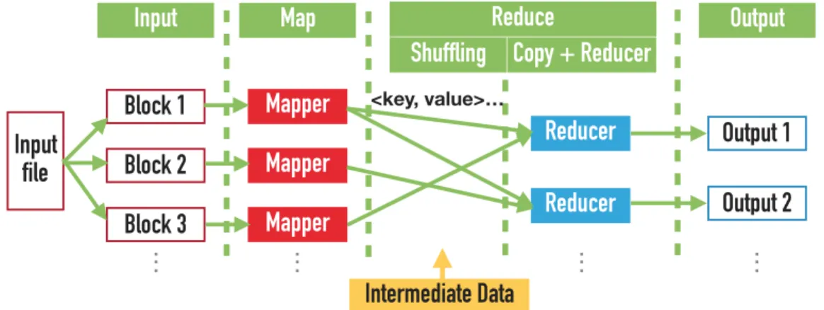
MapReduce is a programming model introduced by Google for processing large data sets on clusters of computers. Fig. 2.1 shows the parallel data processing scheme of MapReduce. A typical MapReduce job contains two stages: map and reduce. Each stage consists of multiple identical tasks. A map task (mapper) processes one block of the raw data which is stored in a shared distributed file system and generates intermediate data in a form of <key, value>. There are three components in the reduce stage: shuffling, copy and reducer. Shuffling is responsible for copying inter-mediate data from the map phase to the reduce phase. Once shuffling finishes all the intermediate data transfer, copy component collects data and the reducer component processes the intermediate data and produces the final results.

(25)

Input

file

Block 1

Block 2

Block 3

Mapper

Reducer

Output 1

Output 2

Input

Map

Shuffling Copy + Reducer

Reduce

Output

Intermediate Data

<key, value>…

. . .

Figure 2.1: MapReduce data processing scheme.

2.2 Hadoop MapReduce

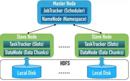
The Apache Hadoop MapReduce is an open source implementation of MapReduce. The structure of Hadoop is shown in Fig. 2.2. In a Hadoop cluster, there is one centralized master node and several distributed slave nodes. Two major components are contained in Hadoop: Hadoop distributed file system (HDFS) and MapReduce job execution system. The local disks from slave nodes are combined together as the distributed file system. All input and output data are split into multiple data blocks and saved separately in it. Each data block can have multiple redundant copies for fault tolerance and data locality. A centralized NameNode deployed in the master node is responsible for the management of HDFS. It stores metadata, file names and block locations. In each slave node, a DataNode module manages the stored data.

In the job execution, users submit applications to the master node. All jobs are scheduled and managed by the JobTracker in the master node. One job consists of multiple map/reduce tasks. The scheduler in the JobTracker is in charge of assigning tasks to the TaskTracker of the appropriate slave nodes, and each TaskTracker is responsible for executing tasks. In each slave node, resources are represented as task slots. TaskTracker manages a number of map/reduce slots that can be used to run either map tasks or reduce tasks. One task slot can execute one task at a time.

(26)

Master Node

JobTracker (Scheduler)

NameNode (Namespace)

Slave Node

TaskTracker (Slots)

DataNode (Data Chunks)

Local Disk

Slave Node

TaskTracker (Slots)

DataNode (Data Chunks)

……

Local Disk

……

HDFS

Figure 2.2: Structure of Apache Hadoop.

Map (resp. reduce) tasks can only run on map (resp. reduce) slots. The number of map/reduce slots in each TaskTracker can be set in the system configuration file. Once the Hadoop cluster is set up, such configuration cannot be changed.

2.3 Hadoop YARN

Hadoop YARN is the next generation of Hadoop. Similar to Hadoop MapReduce, in Hadoop YARN, there is a centralized master node running ResourceManager and several distributed slave nodes deployed by NodeManager on each slave. However, Hadoop YARN has two main differences from the first generation of Hadoop. First, YARN supports fine-grained resource management. Each slave node specifies resource capacity in the format of CPU cores and memory. Each task specifies a resource demand while submitted and ResourceManager responds the resource demand by granting a resource container in a slave node. The second difference is that the resource management and job coordination are separated in YARN. A new component ApplicationMaster takes care of the job coordination. And the ResourceManager is just responsible for scheduling. In this case, YARN can support different frameworks on the same cluster, such as MapReduce and Spark.

(27)

Shown in Fig. 2.3 is the execution of a job in Hadoop YARN. When users submit a job to the ResourceManager, an ApplicationMaster will be launched in a NodeM-anager. Then the ApplicationMaster requests resource for the tasks of the job to the ResourceManager. ResourceManager responses it multiple tokens to the containers. Each token describes the resource a task can get. Within the tokens, Application-Master will launch containers in the NodeManager and assign tasks for execution.

ResourceManager Scheduler …… NodeManager Task Container Task Container ……

Client 1) Submit a job 2) Launch ApplicationMaster

NodeManager ApplicationMasterContainer …… 3) Submit Resource Requests 4) Assign Resource 5) Launch and Coordinate Tasks

Figure 2.3: Job execution in Hadoop YARN

2.4 Typical Scheduling Policies

With a large volume of jobs submitted in a batch by multiple users, resource management and scheduling play an important role on the performance of every job and the overall system. Researchers have put tremendous efforts on job scheduling, resource management, program design, and Hadoop applications [15, 16, 17, 18, 19, 20, 21, 22, 23]. Among them, FIFO, Fair, and Capacity are typical ones that are provided by most of the big data computing systems.

In FIFO scheduling, all jobs are placed in a queue in the order of the submission time. The job submitted first is served first. Once its tasks have been all allocated for execution, the next job in the queue is run. Fair Scheduling aims to allocate fair resource sharing across jobs over time. Priorities and weights may be configured for

(28)

different jobs in resource allocation. Capacity scheduling offers similar functionality as the Fair scheduling. Under Capacity, multiple job queues are defined for different users. The scheduler offers equal resource for each queue while FIFO scheduling is provided for the jobs in the same queue.

Above scheduling policies are default settings in most computing systems such as Hadoop MapReduce, Hadoop YARN and Spark. However, they do not consider the efficiency of resource utilization of the system. In the following chapters, we introduce our resource management schemes and compare the system performance under our approaches with the one under default scheduling policies.

(29)

CHAPTER 3 WORKLOAD-BASED RESOURCE ALLOCATION

In this chapter, we focus on the scheduling problems on resource allocation for different stages of jobs based on their workloads. We proposes a new resource

manage-ment scheme called_FRESH. In_FRESH, we develop a new monitoring component to

detect the run-time workloads of each stage in the cluster. Based on the monitoring results, FRESH dynamically adjusts the resource allocation for different stages in

order to improve the system resource utilization and reduce the makespan of batch jobs. In addition, an improved fairness mechanism inFRESH guarantees that equal

resources are assigned to each running job in the cluster. FRESH is implemented

in Hadoop MapReduce platform but its general mechanism can be easily utilized in other computing systems. The following parts of this chapter indicate the details of _FRESH, including motivation, solution, and the evaluation of _FRESH. We also evaluate the performance of default scheduling policies to show the improvement of

FRESH in both system performance and fairness of applications.

3.1 Background and Motivation

One big challenge for Hadoop users is how to appropriately configure their sys-tems. As a complex system, Hadoop is built with a large set of system parameters. While it provides the flexibility to customize a Hadoop cluster for various applica-tions, it is often difficult for the user to understand those system parameters and set the optimal values for them. In this work, we target on an extremely important Hadoop parameter, slot configuration, and develop a suite of solutions to improve the

(30)

performance, with respect to the makespan of a batch of jobs and the fairness among them.

In a classic Hadoop cluster, each job consists of multiple map and reduce tasks. The concept of “slot” is used to indicate the capacity of accommodating tasks on each node in the cluster. Each node usually has a predefined number of slots and a slot could be configured as either a map slot or a reduce slot. The slot type indicates which type of tasks (map or reduce) it can serve. At any given time, only one task can be running per slot. While the slot configuration is critical for the performance, Hadoop by default uses fixed numbers of map slots and reduce slots at each node throughout the lifetime of a cluster. The values are usually set with heuristic numbers without considering job characteristics. Such static settings certainly cannot yield the optimal performance for varying workloads. Therefore, our main target is to address this issue and improve the makespan performance. Besides the makespan, fairness is another performance metric we consider. Fairness is critical when multiple jobs are allowed to be concurrently executed in a cluster. With different characteristics, each job may consume different amount of system resources. Without a careful plan and management, some jobs may starve while other take advantages and finish the execution much faster. Prior work has studied this issue and proposed some solutions. But we found that the previous work did not accurately define the fairness for this two-phase MapReduce process. In this work, we present a novel fairness definition that captures the overall resource consumption. Our solution also aims to achieve a good fairness among all the jobs.

Specifically, we propose a new approach, “FRESH”, to achieving fair and efficient

slot configuration and scheduling for Hadoop clusters. Our solution attempts to ac-complish two major tasks: (1) decide the slot configuration, i.e., how many map/reduce slots are appropriate; and (2) assign map/reduce tasks to available slots. The targets of our approach include minimizing the makespan as the major objective and

(31)

mean-while improving the fairness without degrading the makespan. _FRESHincludes two models, static slot configuration and dynamic slot configuration. In the first model,

FRESH derives the slot configuration before launching the Hadoop cluster and uses

the same setting during the execution just like the conventional Hadoop. In the sec-ond model,FRESHallows a slot to change its type after the cluster has been started.

When a slot finishes its task, our solution dynamically configures the slot and assigns it the next task. Our experimental results show that FRESHsignificantly improves

the performance in terms of makespan and fairness in the system.

3.2 Problem Formulation

We consider that a user submits a batch of n jobs, J = {J1, J2, . . . , Jn}, to a

Hadoop cluster with S slots in total. Each job Ji containsnm(i) map tasks and nr(i)

reduce tasks. Letsm andsr be the total numbers of map slots and reduce slots in the

cluster, i.e.,S =sm+sr. We assume that an admission control mechanism is in effect

in the cluster such that there is an upper bound limit on the number of jobs that can run concurrently. Specifically, we assume in this work that at any time, there are at mostk jobs running in map phase and at mostk jobs running in reduce phase. Thus, the maximum number of active jobs in the cluster is 2k. Here, k is a user-specified parameter for balancing the trade-off between fairness and makespan. Our objective is to minimize the makespan (i.e., the total completion length) of the job setJ while achieving the fairness among these jobs as well.

To solve the problem, we develop a new scheduling solutionFRESHfor allocating

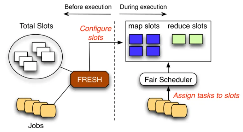
slots to Hadoop tasks. Essentially, we need to address two issues. First, given the total number of slots, how to allocate them for map and reduce, i.e, how many map slots and reduce slots are appropriate. Second, when a slot is available, which task should be assigned to it. FRESH considers two models, i.e., static slot configuration (see

(32)

of map and reduce slots are decided before launching the cluster, similar to the conventional Hadoop system. In this model, we assume that job profiles are available as prior knowledge. Our goal is to derive the best slot setting, thus addressing the first issue. During the execution,Fair scheduleris used to assign tasks to available

slots. In the second model of dynamic slot configuration, FRESH allows a slot to

change its type in an online manner and thus dynamically controls the allocation of map and reduce slots. In addition,FRESH includes an algorithm that assigns tasks

to available slots.

Jobs Total Slots

Fair Scheduler FRESH

map slots reduce slots

Before execution During execution

Assign tasks to slots Conﬁgure

slots

Figure 3.1: Static slot configuration.

Jobs Total Slots

FRESH map slots reduce slots Before execution During execution

Assign tasks to slots Conﬁgure

slots

(33)

3.3 Our Solution: FRESH

In this section, we present our algorithm in_FRESH. It contains two components: static slot configuration and dynamic slot configuration.

3.3.1 Static Slot Configuration

First, we present our algorithm in _FRESH for static slot configuration, where the assignments of map and reduce slots are preset in configuration files and loaded when the Hadoop cluster is launched. Our objective is to derive the optimal slot configuration given the workload profiles of a set of Hadoop jobs.

We assume that the workload of each job is available as prior knowledge. This information can be obtained from historical execution records or empirical estimation. Let ¯tm(i) and ¯tr(i) be the average execution time of a map task and a reduce task of

jobJi. We define wm(i) and wr(i) as the workloads of map tasks and reduce tasks of

Ji, which represent the summation of the execution time of all map tasks and reduce

tasks of Ji. Therefore, wm(i) and wr(i) can be defined as:

wm(i) = nm(i)·¯tm(i), wr(i) = nr(i)·¯tr(i).

Let cm and cr represent the number of slots that a job can occupy to run its map

and reduce tasks. Recall that Fair scheduler is used to assign tasks and each

active job is evenly allocated slots for its tasks. In addition, under our admission control policy, a busy cluster has k jobs concurrently running in map phase and k

jobs concurrently running in reduce phase. Therefore, we have cm and cr defined as

follows: cm = sm k , cr = sr k.

We develop a new algorithm (see Algorithm 3.3.1) to derive the optimal static slot configuration. Our basic idea is to enumerate all possible settings of sm and

(34)

represent the sets of jobs that are currently running in their map phase and reduce phase, respectively. Each element in Mand R is the job index of the corresponding running job. Initially,M={1,2, . . . , k}and R ={}. According to their definitions, when job Ji finishes its map phase, the index i will be moved from M to R. The

sizes of M and R are upper-bounded by the parameter k. Additionally, we use Wi

to represent the remaining workload ofJi in the current phase (either map or reduce

phase). Before Ji enters the map phase, Wi is set to its workload of the map phase

wm(i), i.e., Wi =wm(i). During the execution in the map phase,Wi will be updated

according to the progress. When job Ji finishes its map phase, Wi will be set to its

workload of the reduce phase, i.e., Wi =wr(i).

Algorithm 3.3.1 presents the details of our solution. The outer loop enumerates all possible slot configurations (i.e., sm and sr). For each particular configuration,

we first calculate the workloads of each job’s map and reduce phases, i.e., wm(i) and

wr(i), and set the initial value of Wi (see lines 3–5). In line 6, we initialize some

important variables, where Mand R are as defined above, R0 _{represents an ordered}

list of pending jobs that have finished their map phase, but have not entered their reduce phase yet, andT, initialized as zero, records the makespan of this set of jobs. The core component of the algorithm is the while loop (see lines 7–22) that calculates

the makespan and terminates when both M and R are empty. In this loop, our

algorithm mimics the execution order of all the jobs. Both M and R keep intact

until one of the running jobs finishes its current map (or reduce) phase. In each round of execution in the while loop, our algorithm finds the first job that changes the status and then updates the job sets accordingly. This target job could be in

either map or reduce phase depending on its remaining workload and the number

of slots assigned to each job. In Algorithm 3.3.1, lines 8–9 find two jobs (Ju and

Jv) which have the minimum remaining workloads in M and R, respectively. These

(35)

cr represent the number of slots assigned to each of them under Fair scheduler

scheduling policy. Thus, the remaining execution times for Ju and Jv to complete

their phases are Wu

cm and

Wv

cr , respectively.

If Ju finishes its map phase first (the case in lines 10–16), then we remove u

fromM, update the current makespan, and set the remaining workload of Ju to the

workload of its reduce phase (line 11). We also update the remaining workloads of all other active jobs in M and R (lines 12–13). In addition, the algorithm picks a new job to enter its map phase in line 14. Finally, we add u toR to start its reduce phase if the capacity limit of R is not reached. Otherwise, u is added to the tail of the pending listR0 _{(lines 15–16).}

The function DeductWorkload is called to update the remaining workloads for

active jobs inMor R. As shown below, the inputs of this function include a job set

A (e.g., M, R) and the value of the completed workload w. The remaing workload of each job i in A is then updated by deducting w.

function DeductWorkload(A,w){

/*A: a set of job IDs,w: a workload value */

for i∈ A do Wi ←Wi−w end }

Once jobJv finishes its reduce phase (see the other case in lines 17–21), we update

the current makespan as well as the remaining workloads of all other active jobs in

M and R. Similarly, index v is removed from R. If R0 _{is now not empty, then}

the first job in R0 _{will be moved to} _R_{. At the end, in lines 22–23, the algorithm}

compares the present makespan T to the variable Opt M S which keeps track of the

minimum makespan, and updates Opt M S if needed. Another auxiliary variable

Opt SM is used to record the corresponding slot configuration. The time complexity of Algorithm 3.3.1 is O(S·N2

T), where NT = P_i(nm(i) +nr(i)) is the total number

(36)

is quite small. For example, with 500 slots and 100 jobs each having 400 tasks, the computation overhead is 0.578 seconds on a desktop server with 2.4GHz CPU.

Algorithm 3.3.1: Static Slot Configuration 1: for sm = 1 to S do 2: sr =S−sm 3: for i= 1 to n do 4: wm(i) =nm(i)·¯tm(i), wr(i) =nr(i)·t¯r(i) 5: Wi =wm(i) 6: end for 7: M={1,2, . . . , k},R={},R0 ₌_{}_{, T} _{= 0} 8: while MS R 6=φ do 9: u= arg min_i_∈MWi, cm = _|M|sm 10: v = arg min_i_∈RWi, cr = _|R|sr 11: if Wu cm < Wv cr then 12: M ← M −u, T =T + Wu cm, Wu =wr(u) 13: DeductWorkload(M, wm(u)) 14: DeductWorkload(R,wm_c(u) m ·cr)

15: pick a new job from J and add its index to M

16: if|R| < k then R ← R+u

17: else add u to the tail of R0

18: else 19: R ← R −v, T =T +Wv cr 20: DeductWorkload(R, Wv) 21: DeductWorkload(M,Wv cr ·cm) 22: if|R0_|_>₀ _then _move _R0_{[0] to} _R 23: end if 24: end while

25: ifT < Opt M S then Opt M S =T, Opt SM =sm

26: end for

27: return Opt SM and Opt M S

3.3.2 Dynamic Slot Configuration

Then we turn to discuss the model in FRESH for dynamic slot configuration.

The critical target of this model is to enable a slot to change its type (i.e., map or reduce) after the cluster is launched. To accomplish it, we develop solutions for both configuring slots and assigning tasks to slots. In addition, we redefine the fairness of resource consumption among jobs. Therefore, our goal is to minimize the makespan of

(37)

jobs while achieving the best fairness without degrading the makespan performance. The rest of this section is organized as follows. We first introduce the new overall fairness metric. Then we present the algorithm for dynamically configuring map and reduce slots. Finally, we describe how FRESH assigns tasks to the slots in the

cluster.

3.3.2.1 Overall Fairness Measurement

Fairness is an important performance metric for our algorithm design. However, the traditional fairness definition does not accurately reflect the total resource con-sumptions of jobs. In this subsection, we present a new approach to quantify fairness measurement, where we define the resource usage in MapReduce process and use Jain’s index [24] to represent the level of fairness.

In a conventional Hadoop system, Fair scheduler evenly allocates the map

(resp. reduce) slots to active jobs in their map (resp. reduce) phases. Although the fairness is achieved in map and reduce phases separately, it does not guarantee the fairness among all jobs when we combine the resources (slots) consumed in both map and reduce phases. For example, assume a cluster has 4 map slots and 4 reduce slots running the following 3 jobs: J1 (2 map tasks and 9 reduce tasks), J2 (3 map tasks and 4 reduce tasks), and J3 (7 map tasks and 3 reduce tasks). Assume every task can be finished in a unit time. The following table shows the slot assignment with

Fair scheduler at the beginning of each time point (‘M’ and ‘R’ indicate the type

of slots allocated for the jobs). Eventually, all three jobs are finished in 5 time units. However, they occupy 11, 7, and 10 slots respectively.

0 1 2 3 4

J1 2(M) 4(R) 2(R) 1(R) 2(R)

J2 1(M) 2(M) 2(R) 1(R) 1(R)

(38)

In this work, we define a new fairness metric, named overall fairness, as follows. At any time point T, let J0 represents the set of currently active jobs in the system, and Ti represents the starting time of job Ji in J0. We use two matrices tm[i, j] and

tr[i, j] to represent the execution times of jobJi’sj-th map task andj-th reduce task,

respectively. Note that these two matrices include the unfinished tasks. Therefore, the resources consumed by job Ji by time T can be expressed as

ri(T) = P jtm[i, j] + P jtr[i, j] T −Ti . (3.1)

where the above formula represents the effective resources Ji has consumed during

the period ofT −Ti. The bigger ri(T) is, the more resources Ji has been assigned to.

In addition, we use Jain’s index on ri to indicate the overall fairness (F(T)) at the

time point T, i.e.,

F(T) = ( P iri(T))2 |J0_|P iri2(T) ,

where F(T)∈[_|_J10_|,1] and a larger value indicates better fairness.

3.3.2.2 Configure Slots

The function of configuring slots is to decide how many slots should serve map/reduce tasks based on the current situation. Specifically, when a task is finished and a slot is freed, our system needs to determine the type of this available slot in order to serve other tasks. In this subsection, we present the algorithm in _FRESH that appropri-ately configures map and reduce slots.

First of all, our solution makes use of the statistical information of the finished tasks from each job. This information is available in Hadoop system variables and log files. Let ¯tm(i) and ¯tr(i) be the average execution times of job Ji’s map task

and reduce task, respectively. Once a task completes, we can access its execution time and then update ¯tm(i) or ¯tr(i) for job Ji which that particular task belongs

(39)

to. In addition, we use n0_m(i) and n0_r(i) to indicate the number of remaining map tasks and reduce tasks, respectively, in job Ji. Theremaining workload of a job Ji is

then defined as follows: w0_m(i) =n0_m(i)·_t¯_m₍_i₎_{, w}0

r(i) =n

0

r(i)·¯tr(i), where wm0 (i) isJi’s

remaining map workload and w0_r(i) is the remaining reduce workload of Ji. Finally,

we estimate the total remaining workloads of all the pending map and reduce tasks. LetRWm represents the summation of all the remaining map workloads of jobs inM

while RWr represents the summation of all the remaining reduce workloads for jobs

inR and R0_. _RW

m and RWr can be calculated as:

RWm = X i∈M w0_m(i), RWr = X i∈RS R0 w_r0(i).

Note that RWm includes the jobs running in their map phases (in M) while RWr

includes the jobs running in their reduce phases (in R) as well as the jobs that have finished their map phases but wait for running their reduce phase (in R0_).

The intuition of the algorithm in _FRESHis to keep jobs in their map and reduce phases in a consistent progress so that all jobs can be properly pipelined to avoid waiting for slots or having idle slots. Therefore, the numbers of map and reduce slots should be proportional to the total remaining workloads RWm and RWr, i.e.,

the heavier loaded phase gets more slots to serve its tasks. However, this idea may not work well in the map-reduce process because there could be a sudden change on the remaining workloads. The problem arises when a job finishes its map phase and enters the reduce phase. Based on the definition of RWm and RWr, this job will

bring its reduce workload to RWr and a new job which starts its map phase then

add its new map workload to RWm. Such workload updates, however, could greatly

change the weights of RWm and RWr. For example, if RWm >> RWr, most of slots

are map slots. Assume a reduce-intensive job just finishes its map phase and incurs a lot of reduce workload, the system has no sufficient reduce slots to serve the new reduce tasks. It takes some time for the cluster to adjust to this sudden workload

(40)

change as it has to wait for the completions of many map tasks before configuring those released slots to be reduce slots.

We develop Algorithm 3.3.2 to derive the optimal slot configuration in an online mode. We follow the basic design principal with a threshold-based control to mitigate the negative effects from those sudden changes in map/reduce workloads. When a map/reduce task is finished, the algorithm collects the task execution time and updates a set of statistical information including the average task execution time, the number of remaining tasks, the remaining workload of job Ji, and the total

remaining workloads (see lines 1–4). Following that, the algorithm calls a function, calledCalExpSm, to calculate the expected number of map slots (expSm) based on the current statistical information. If the expectation is more than the current number of map slots (sm), this free slot will become a map slot. Otherwise, we set it to be a

reduce slot.

Algorithm 3.3.2: Configure a Free Slot 1: if a map task of job Ji is finished then

2: update ¯tm(i),n0m(i),w0m(i) andRWm

3: end if

4: if a reduce task of jobJi is finished then

5: update ¯tr(i),n0r(i), w0r(i) and RWr

6: end if

7: expSm=CalExpSm()

8: if expSm > sm then set the slot to be a map slot

9: else set the slot to be a reduce slot

The details of the functionCalExpSmare presented in Algorithm 3.3.3. We useθcur

to represent the expected ratio of map slots based on the current remaining workload. In line 2, we choose an active job Ja which has the minimum map workload, i.e., job

Jais supposed to first finish its map phase. If Ja is still far from the completion of its

map phase, then the risk of having a sudden workload change is low and the function just returnsθcur·Sas the expected number of map slots. We set a parameterτ1as the progress threshold. When jobJa is close to the end of its map phase, i.e., the progress

(41)

exceedsτ1, the function will consider the potential issue with the sudden change of the workload (lines 6–13). Essentially, the function tries to estimate the map and reduce workloads when Ja enters its reduce phase, and calculate the expected ratio of map

slots θexp at that point. A sudden change of the workload happens whenθexp is quite

different from the ratio of map slotsθcur we get based on the current configuration. In

the case that a sudden change is predicted, we will useθexp·Sinstead as the guideline

for new slot configuration. Otherwise, the function still returns θcur·S.

Specifically in Algorithm 3.3.3, when Ja finishes its remaining map workload

w0_m(a), we assume the other jobs inM have made roughly the same progress. Thus the total map workload will be reduced byw0_m(a)·k. Then a new job will join the set

M, let it be job Jb, and wm(b) will be added to the total remaining workload RWm

(line 7). Meanwhile, Ja will belong to either set R or R0 and its reduce workload

wr(i) will be added to the total remaining reduce workload RWr (line 8). Variable

θexp in line 9 denotes the expected ratio of map slots at that point. Next, the

func-tion estimates the number of map slots following the configurafunc-tion ratioθcur whenJa

finishes its map phase. It involves the number of slots freed from the current point. It is apparent that there is no other map slot released based on the definition of Ja,

thus we just need to estimate the number of available reduce slots during this period. In Algorithm 3.3.3, we use η to represent this number and estimate its value based on the following Theorem 3.3.1. In line 11, we predict the number of map slots s0_m

using the current configuration ratio, i.e., η·θcur slots will become map slots.

Even-tually, the function compares the estimated ratio to the expected ratio in line 12. If the difference is over a threshold τ2, we will consider the future expected ratio θexp.

Otherwise, we will continue to use the current configuration ratioθcur.

Theorem 3.3.1 Assume reduce tasks are finished at a rate of one per r time units, the number (η) of available reduce slots whenJa finishes its remaining map workload

(42)

Algorithm 3.3.3: FunctionCalExpSm() 1: θcur = _RWRW_m₊m_RW_r

2: a= arg min_i_∈Mw_m0 (i)

3: if the progress of jobJa< τ1 then

4: returnθcur·S

5: else

6: Let job Jb be the next that will start its map phase

7: RW_m0 =RWm−w0m(a)·k+wm(b)

8: RW_r0 =RWr+wr(a)

9: θexp =RWm0 /(RWr0+RWm0 )

10: calculate η using Theorem 3.3.1

11: s0_m =sm+θcur·η

12: if |

s0_m

S −θexp|

θexp > τ2 then returnθexp·S 13: else returnθcur·S

14: end if η= p m2 a+ 4·c·w0m(a)−ma 2·c·r . where c = θcur 2·r·k, w 0

m(a) indicates the remaining map workload of Ja, and ma is the

number of map slots assigned to Ja.

Proof Assume jobJa will finish its remaining map workload wm0 (a) in x time units.

According to our assumption, a reduce task will be finished everyrtime units. There-fore, whenJa finishes its map phase, there will beη = x_r reduce slots released as well.

Assume that we use θcur to allocate slots and k jobs in Mare evenly assigned newly

released slots. Job Ja will continuously obtain x·_rθ_·cur_k new map slots. It is equivalent

to having half of them x·θcur

2·r·k from the beginning. Therefore, the remaining time for

Ja to finish the map phase can be estimated as

x=w0_m(a)/(x·θcur

2·r·k +ma),

where ma is the number of map slots currently assigned toJa. By solving the above

equation, we have x= p m2 a+ 4·c·wm0 (a)−ma 2·c .

(43)

Thus: η= p m2 a+ 4·c·w0m(a)−ma 2·c·r .

3.3.2.3 Assign Tasks to Slots

Once the type of the released slot is determined, FRESH will assign a task to

that slot. Basically, we need to select an active job and let the available map/reduce slot serve a map/reduce task from that job. In FRESH, we follow the basic idea

in Fair scheduler but use the new overall fairness metric instead: calculate the

resource consumption for each job based on Eq.(3.1) and choose the job with the most deficiency ofoverall fairness.

Algorithm 3.3.4: Assign a Task to a Slot

1: Initial: C ={}, now ← current time in system 2: if the slot is configured for map tasksthen C ← M

3: else C ← R

4: for each job Ji ∈ C do

5: totali = 0

6: for each task j in job Ji do

7: if task j is finished then ej ←fj −sj

8: else if taskj is running then ej ←now−sj

9: else ej ←0 10: totali =totali+ej 11: end for 12: ri = _nowtotal₋i_T i 13: end for

14: s= arg min_i_∈Ari

15: assign a task of job Js to the slot

Algorithm 3.3.4 illustrates our solution in _FRESH for assigning a task to an available slot. We use C to indicate a set of candidate jobs. Initially, C is empty and we use variable now to indicate the current time. When a slot is configured to serve map tasks (using Algorithm 3.3.2), C is a copy of M. Otherwise, C is a copy of R

(lines 2–3). The outer loop (lines 4–11) then calculates the resource consumption for each job in C at the current time. Variable totali, initialized as 0 in line 5, is used

(44)

to record the total execution time for all finished and running tasks in job Ji (lines

6–10). We useej to denote the execution time of task j. If task j has been finished,

its execution time ej is the difference between its finish time fj and its start time sj

(line 7). If task j is still running, then ej is equal to the current time now deducted

by its start time sj (line 8). Once the total execution time for job Ji is obtained,

we get the resources consumption ri by normalizing the total execution time totali

by the duration between the current time and the start time of job Ji (Ti), as shown

in line 11. Finally, the job with the minimum resource consumption is chosen to be served by the available slot.

3.4 Performance Evaluation

In this section, we evaluate the performance of FRESHand compare it with other

alternative schemes. We use FRESH-static and FRESH-dynamic to represent our

static slot configuration and dynamic slot configuration respectively.

3.4.1 Experimental Setup and Workloads

First, we introduce our implementation details, the cluster setting and the work-load for the evaluation.

Implementation

We have implemented FRESH on Hadoop version 0.20.2. For FRESH-static,

we develop an external program to derive the best slot setting and apply it to the Hadoop configuration file. The Hadoop system itself is not modified for FRESH

-static. To implement FRESH-dynamic, we have added a few new components to

Hadoop. First, we implement the admission control policy with the parameterk, i.e., at most k jobs are allowed to be concurrently running in map phase or in reduce phase. Second, we create two new modules in J obT racker. One module updates the statistical information such as the average execution time of a task, and estimates

(45)

the remaining workload of each active job. The other module is designed to configure a free slot to be a map slot or a reduce slot and assign a task to it according to the algorithms in section 3.3.2. The two threshold parameters in Algorithm 3.3.3 are set as τ1 = 0.8 and τ2 = 0.6. We have tested with different values and found that the performance is close when τ1 ∈ [0.7,0.9] and τ2 ∈ [0.5,0.7]. Due to the page limit, we omit the discussion about these two heuristic values. In addition, job profiles (execution time of tasks) are generated based on the experimental results when a job is individually executed. However, we randomly introduce±30% bias to the measured execution time and use them as the job profiles representing rough estimates.

3.4.1.1 Hadoop Cluster

All the experiments are conducted on Amazon AWS cloud computing platform. We create a Hadoop clusters consisting of 11 m1.xlarge Amazon EC2 instances [25], one master node and 10 slave nodes. Each node is set to have 4 slots since an m1.xlarge instance at Amazon EC2 has 4 virtual cores. Totally, there are S = 40 slots in the cluster. In addition, to represent the scalability of FRESH, Fig. 3.10 shows a set of experiments in a larger cluster which doubles the slave nodes, i.e., one master node and 20 slave nodes withS = 80 slots totally.

3.4.1.2 Workloads

Our workloads for evaluation consider general Hadoop benchmarks with large datasets as the input. In particular, four datasets are used in our experiments includ-ing 4GB/8GB wiki category links data, and 4GB/8GB movie ratinclud-ing data. The wiki data includes the information about wiki page categories and the movie rating data is the user rating information. We choose the following six Hadoop benchmarks from Purdue MapReduce Benchmarks Suite [26] to evaluate the performance.

• Classif ication: Take the movie rating data as input and classify the movies based on their ratings.

(46)

• Invertedindex: Take a list of Wikipedia documents as input and generate word to document indexing.

• W ordcount: Take a list of Wikipedia documents as input and count the occur-rences of each word.

• Grep: Take a list of Wikipedia documents as input and search for a pattern in the files.

• Histogram Rating: Generate a histogram of the movie rating data (with 5 bins).

• Histogram M ovies: Generate a histogram of the movie rating data (with 8 bins).

3.4.2 Performance Evaluation

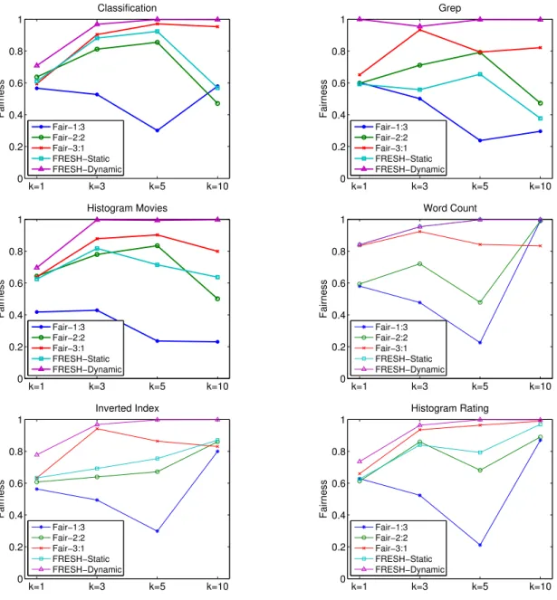
In this subsection, we present the performance of FRESH and compare to other solutions. Given a batch of MapReduce jobs, our major performance metrics are makespan, i.e., the finish time of the last job, and fairness among all jobs. We mainly

compare to the conventional Hadoop system with the _{Fair scheduler} and static

slot configuration. In our setting, each slave has 4 slots, thus there are three possible static settings in conventional Hadoop, 1 map slot/3 reduce slots, 2 map slots/2 reduce slots, and 3 map slots/1 reduce slot. We use Fair-1:3, Fair-2:2, and Fair-3:1

to represent these three settings respectively.

We have conducted two categories of tests with different job workloads, simple workloads consist of the same type of jobs (selected from the six MapReduce bench-marks), and mixed workloads represent a set of hybrid jobs. In the reset of this subsection, we separately present the evaluation results with these two categories of workloads.

(47)

3.4.2.1 Performance with Simple Workloads

For testing simple workloads, we generate 10 Hadoop jobs for each of the above 6 benchmarks. Every set of 10 jobs share the same input data set and they are consecutively submitted to the Hadoop cluster with an interval of 2 seconds. In addition, we have tested different values of k to show the effect of the admission control policy, particularly k = 1,3,5,10.

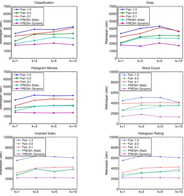
Fig. 3.3 shows the performance of the makespan. First, we observe that in conven-tional Hadoop, the best performance is achieved mostly whenk = 1, i.e., only one job in map and reduce phase which is equivalent to FIFO(First-In-First-Out) scheduler. It indicates that while improving the fairness, the _{Fair scheduler} sacrifices the makespan of a set of jobs. The major cause is the resource contention among jobs which prolongs the execution of each task. Our solution, FRESH-static performs no worse than the best setting with Fair scheduler. In some workload such as

“Clas-sification”, the improvement is adequate. In addition, FRESH-dynamic always yields a significant improvement in all the tested settings. For example, FRESH-Dynamic

improves in average about 32.75% in makespan compared to the _{Fair scheduler}

with slot ratio 2:2. In addition, our dynamic slot configuration mitigates the effect of different values of k, thus holding a relatively flat curve in Fig. 3.3.

Fig. 3.4 shows the overall fairness designed in section. 3.2 during the same ex-periments. In most of the cases, the fairness value is a increasing function on k. Especially when k = 10, where all jobs are allowed to be concurrently executed (no admission control), almost all settings obtain a good fairness value. Since all jobs are from the same benchmark in simple workload, they finish their map phases in wave

and enter the reduce phase roughly in the same time. Thus the _{Fair scheduler}

performs well in this case (k=10). Overall, FRESH-Dynamic outperforms all other schemes and achieves very-close-to-1 fairness value even when k = 3 ork = 5.

Building Efficient Large-Scale Big Data Processing Platforms

University of Massachusetts Boston

ScholarWorks at UMass Boston

Building Efficient Large-Scale Big Data Processing

Platforms

Jiayin Wang

BUILDING EFFICIENT LARGE-SCALE BIG DATA PROCESSING

PLATFORMS

BUILDING EFFICIENT LARGE-SCALE BIG DATA PROCESSING

PLATFORMS

ABSTRACT

BUILDING EFFICIENT LARGE-SCALE BIG DATA PROCESSING

PLATFORMS

ACKNOWLEDGMENTS

TABLE OF CONTENTS

LIST OF FIGURES

LIST OF TABLES

CHAPTER 1

INTRODUCTION

Spark

HDFS

Hadoop Distributed File System

Hadoop YARN

Hadoop MapReduce

Mesos

Tez

Hive

Pig

Shark

Storm

Mahout

1.1

Research Challenges

1.2

Dissertation Contributions

1.3

Dissertation Organization

CHAPTER 2

BACKGROUND

2.1

MapReduce

Input

file

Block 1

Block 2

Block 3

Mapper

Mapper

Mapper

Reducer

Reducer

Output 1

Output 2

Input

Map

Shuffling Copy + Reducer

Reduce

Output

Intermediate Data

. . .

. . .

. . .

. . .

2.2

Hadoop MapReduce

Master Node

JobTracker (Scheduler)

NameNode (Namespace)

Slave Node

TaskTracker (Slots)

DataNode (Data Chunks)

Local Disk

Slave Node

TaskTracker (Slots)

DataNode (Data Chunks)

……

Local Disk

……

HDFS

2.3