PRICE STICKINESS AND CUSTOMER ANTAGONISM *

PRICE

STICKINESS

AND

CUSTOMER

ANTAGONISM

Eric

T.

Anderson

and

Duncan

I.

Simester

Managers often state that they are reluctant to vary prices for fear of “antagonizing customers.”   

However, there is no empirical evidence that antagonizing customers through price adjustments 

reduces demand or profits.  We use a 28‐month randomized field experiment involving over 

50,000 customers to investigate how customers react if they buy a product and later observe 

the same retailer selling it for less.  We find that customers react by making fewer subsequent 

purchases from the firm.  The effect is largest among the firm’s most valuable customers: those 

whose prior purchases were most recent and at the highest prices.     

JEL: E3, D12, E44, C93   

Keywords: price stickiness, price adjustments, customer antagonism, field experiments 

*

 We thank Nathan Fong for valuable research assistance and the anonymous retailer for generously 

providing the data used in this study.  We acknowledge valuable comments from Martin Eichenbaum, 

Aviv Nevo, Julio Rotemberg, Catherine Tucker, Birger Wernerfelt, Juanjaun Zhang and numerous other 

colleagues.  The paper has also benefited from comments by seminar participants at Chicago, Columbia, 

Cornell, Erasmus, INSEAD, LBS, Minnesota, MIT, NYU, Northeastern, Northwestern, Penn State, UCLA, 

UCSD, UTD, Yale, the University of Houston, the 2006 Economic Science Association conference, the 2007 

“It seems essential, therefore, to gain a better understanding of precisely what 

firms mean when they say that they hesitate to adjust prices for fear of 

antagonizing customers.”  

    Blinder et al. (1998 page 313) 

I. Introduction

The assumption that nominal prices are sticky is fundamental to Keynesian economics and forms 

a basic premise of many models of monetary policy.  A leading explanation for why prices are 

slow to adjust is that firms do not want to antagonize their customers.  While it has been argued 

that price adjustments may antagonize customers, there is little empirical evidence that this 

affects demand or profits.  In this paper we study how downward price adjustments can lead to 

lower demand and lost profits.  We show that many customers stop purchasing if they see a firm 

charge a lower price than they previously paid for the same item.  This customer boycott is 

concentrated among the firm’s most valuable customers, which greatly magnifies the cost to the 

firm.  Firms can mitigate these costs by limiting the frequency and/or depth of price 

adjustments.   

The findings are replicated in two separate field experiments conducted in different product 

categories.  The first experiment was conducted with a publishing company.  Customers were 

randomly chosen to receive a test or control version of a catalog (the “Test Catalog”).  The 

versions were identical except that the test version offered substantially lower prices on 36 

items (the “Test Items”).  The loss of demand and profits was particularly dramatic among 

customers who had recently paid a higher price for one of those items.  Lower prices in the test 

condition led to 14.8% fewer orders over the next 28‐months, which equates to over $90 in lost 

Decomposing the results reveals that the price adjustments had two effects.  As expected, 

orders from the Test Catalog were higher in the test condition as some customers took 

advantage of the discounted prices.  However, this short‐run effect was overwhelmed by a 

sharp reduction in orders from other catalogs.  Price adjustments in a single catalog had 

negative spillover effects on future orders (and overall revenue).     

To investigate the robustness and generalizability of the results we replicate the key findings 

with a separate company in a different product category (clothing).  This replication is 

particularly noteworthy as most customers expect to see lower prices on clothing at the end of a 

season.  Despite this, we show that sending a “Sale” catalog to customers in the days 

immediately after Christmas reduced purchases by customers who had previously paid a higher 

price for one of the discounted items.    

Although the findings confirm that price adjustments can lower demand and profits, we 

recognize that there may be multiple explanations for this effect.  One explanation is that 

customers are antagonized if they observe the firm charging lower prices than what they 

previously paid.  Another explanation is that lower prices may have prompted customers to 

update their price expectations and change their purchase behavior.  A third possibility is that 

low prices may have influenced customers’ beliefs about product quality.     

To evaluate these explanations we exploit heterogeneity in the experimental treatment effects.  

For example, the reduction in demand and profits was restricted to customers who had recently 

antagonism is consistent with these boundaries.  We also find some evidence that customers 

updated their price expectations and delayed purchasing.  However, this does not appear to 

fully explain the decrease in demand.     

Other explanations are ruled out by the randomized allocation of customers to the two 

experimental conditions.   For example, the randomization ensures that competitive reactions, 

inventory constraints, macroeconomic changes and customer characteristics cannot explain the 

decrease in demand.   These factors were equally likely to affect sales in both conditions.     

The results of the field experiments had a direct impact on the pricing policies of the two 

participating retailers.  After learning of the results, the company that provided data for our first 

experiment responded by no longer sending catalogs containing discounts to customers who 

had recently purchased one of the discounted items.  This effectively reduced the degree to 

which prices are varied to an individual customer.  The company that participated in the second 

study also responded by restricting price changes.  For example, the company removed a 

discounted item from the back page of a widely circulated catalog to avoid antagonizing 

approximately 120,000 customers who had previously purchased the item at full price.  Even 

before learning of the findings, this company had policies that limited the frequency of 

discounts.  Managers acknowledged that these policies reflected concern that frequent price 

adjustments may antagonize customers.     

These reactions suggest that firms may be able to mitigate the reduction in demand by charging 

different prices to different customers.  If the products are durables that most customers only 

retailers are not able to price discriminate as perfectly as the two catalog retailers in this study.  

When firms cannot charge different prices to individual customers the effects that we report will 

tend to reduce the optimal frequency and/or depth of price adjustments.   

Previous Research  

The research on price stickiness can be broadly categorized into two topics: (1) are prices sticky; 

and (2) why are they sticky?  The evidence that prices respond slowly to business cycles is now 

extensive (Gordon 1990; Weiss 1993).  In recent years much of the attention has turned to the 

second question.  One set of explanations argue that costs may be constant, either within a 

limited neighborhood or within a limited time period.  Another common explanation studies the 

(menu) cost of changing prices.  The more costly it is to change prices the less frequently we 

would expect them to change.  Other explanations have considered imperfections in the 

information available to price setters and asymmetries in the demand curve.     

In this paper we study the role of customer antagonism.  This explanation argues that firms do 

not want to change prices as doing so may antagonize their customers.  Hall and Hitch (1939) 

were among the first to empirically investigate this issue.  They interviewed a sample of 

managers to learn how prices are set.  The managers’ responses included statements such as: 

“Price changes [are] a nuisance to agents, and disliked by the market,” and “Frequent changes 

of price would alienate customers,” (pages 35 and 38).  More recently, Blinder, Canetti, Lebow 

and Rudd (1998) also asked managers why they did not vary their prices.  This study was 

conducted on a large scale and involved 200 interviews with senior executives conducted over a 

two year period.  The most common response was that frequent price changes would 

to better understand the role of customer antagonism (pages 85 and 308, see also the 

introductory quote at the start of this paper).  The findings have since been corroborated by 

similar studies surveying managers in Canada (Amirault, Kwan and Wilkinson 2004) and a broad 

range of European countries (Hall, Walsh and Yates 1997; Fabiani et al. 2004; Apel, Friberg and 

Hallsten 2005).1  While these studies have raised awareness that customer antagonism may 

contribute to price stickiness, there are limits to what can be learned from survey data.  Notably, 

the data does not allow researchers to measure whether antagonizing customers through price 

adjustments reduces demand or profits.     

The evidence in this paper is related to Rotemberg’s theoretical research on firm altruism.  

Customers in Rotemberg’s models only want to transact with firms that are “altruistic.”  

Although customers interpret firms’ actions generously, they boycott firms when there is 

convincing evidence that their expectations regarding altruism are violated.  This reaction has 

been used to help explain why prices are sticky (Rotemberg 2005); investigate how customers 

react to brand extensions (Rotemberg 2008); and explore how fairness influences firms’ pricing 

decisions (Rotemberg 2004).  We will present evidence that the reductions in future purchases 

do not just reflect changes in customers’ expectations about prices or product quality.  Instead, 

the effects appear to influence how customers view less tangible characteristics of the firm and 

its brand.  This evidence may be seen as direct support for Rotemberg’s claim that customers’ 

perceptions of whether firms are altruistic contribute to the value of a firm’s brand (Rotemberg 

2008).    

1

 Other empirical evidence includes Zbaracki et al. (2004), who report findings from an extensive study of 

the cost of changing prices at a large industrial firm.  Their findings include a series of anecdotes and 

While our findings are clearly consistent with Rotemberg’s models, this is not the only 

explanation for why customers may stop purchasing from a firm when they are antagonized by 

price adjustments.   It is possible that firms are simply risk averse and want to minimize the risk 

of future antagonism.2  Other explanations are also suggested by previous research on the role 

of reputations and firm brands (Wernerfelt 1998; Tadelis 1999).     

Customer Antagonism When Prices Increase 

We measure the response to downward price adjustments.  This is a natural place to start as it 

invokes a strong strawman: lower prices lead to higher sales.  There is a complementary stream 

of research that studies customer antagonism in response to upwards price adjustments.  The 

origins of this work can be traced to Phelps and Winter (1970) and Okun (1981).  Okun 

introduces the label “customer markets” to describe markets with repeated transactions.  He 

argues that if price increases antagonize buyers, then sellers may respond to unobserved price 

shocks by absorbing the cost changes rather than increasing their prices.   Nakamura and 

Steinsson (2008) extend this intuition in a recent paper.  In their model, price rigidity serves as a 

partial commitment device, which enables sellers to commit not to exploit customers’ 

preferences to repeatedly purchase from the same seller.  The commitment mechanism is 

endogenous and relies on the threat that a deviation would trigger an adverse shift in customer 

beliefs about future prices.3     

As support for their model, Nakamura and Steinsson (2008) cite two experimental papers.   

Renner and Tyran (2004) demonstrate that when buyers are uncertain about product quality 

2

 We thank an anonymous reviewer for this suggestion. 

3 _{In a related paper, Kleshchelski and Vincent (2009) investigate how customer switching costs create an} 

incentive for firms to build market share.  They demonstrate that this may prompt firms to absorb a 

then sellers are less likely to raise prices in response to cost increases if there is an opportunity 

to develop long‐term relationships.  This effect is particularly pronounced if buyers cannot 

observe the cost increases.  The explanation offered for these effects is that the sellers are 

willing to absorb the additional costs rather than risk antagonizing the buyers.  These results 

complement an earlier experimental study (Cason and Friedman 2002) that investigates how 

variation in customers’ search costs affects both their willingness to engage in repeated 

relationships and the resulting variation in prices.  The authors show that higher search costs 

tend to result in more repeated relationships, increasing sellers’ profits and leading to less 

variation in prices.     

Other Relevant Research 

Our findings are also related to previous work on intertemporal price discrimination.   Research 

on the timing of retail sales argues that firms can profit by occasionally lowering prices and 

selling to a pool of low‐valuation customers (Conlisk, Gerstner and Sobel 1984; Sobel 1984, 

1991).  These arguments do not consider the possibility that customers who observe the lower 

prices may be less likely to make future purchases.  Our findings represent a countervailing force 

that may limit a firm’s willingness to price discriminate.     

The findings are also relevant to recent work on price obfuscation.  This literature recognizes 

that many firms adopt practices that make it difficult for customers to compare prices (Ellison 

and Ellison 2009; Ellison 2006).  Price obfuscation may allow firms to mitigate the reactions that 

we document in this paper.  If customers cannot easily compare prices then we would not 

expect the same outcomes.  In this respect, our findings may help to explain the use of price 

Finally, we can also compare our findings with research on reference prices (Kahneman, Knetsch 

and Thaler 1986).  A challenge in the reference price literature is to identify the correct 

“reference” price.  Some customers may use later prices as a reference against which to 

evaluate the price paid in earlier transactions.  Under this interpretation, the findings are easily 

reconciled with the reference price literature: customers who later see the firm charging a lower 

price may conclude they experienced a loss from overpaying in the past.  We caution that this 

definition of the reference price is not unique, and alternative definitions may lead to different 

predictions.   

Plan of the Paper 

The paper continues in Section 2 with a detailed description of the experimental setting and the 

design of the first field experiment.  We present initial findings in Section 3, which provide both 

context and motivation for the results that follow.   We investigate how the outcome is 

moderated by the recency of customers’ prior purchases in Section 4.  In Section 5 we consider 

the price paid in the prior purchases, together with the persistence of the results across the 28‐

month measurement period.   In Section 6 we investigate three alternative explanations for the 

results, and then in Section 7 we present a replication in a different product category. The paper 

concludes with a summary of the findings and limitations in Section 8.   

II. Study Design

The primary field experiment was conducted with a medium‐sized publishing retailer that 

customers.4  All of the products carry the retailer’s brand name and are sold exclusively through 

the company’s catalogs.  At the time of our study the firm also operated an Internet site, but 

few customers placed their orders online. The products are durables with similar characteristics 

to books, computer software and music.  It is rare for customers to buy multiple units of the 

same item (few customers buy two copies of Oliver Twist) and so incremental sales typically 

reflect purchases of other items (buying both Oliver Twist and David Copperfield).  The average 

inter‐purchase interval is 48‐weeks.    

Interviews with managers revealed that the firm engages in inter‐temporal price discrimination, 

charging relatively high regular prices interspersed with frequent shallow discounts and 

occasional deep discounts.  A review of the firm’s historical transaction data confirms that there 

had been wide variation in prices paid for the same item.  Approximately one fifth of 

transactions occur at the regular price, with most of the remaining transactions occurring at 

either a shallow (20%‐30%) or deep (50%‐60%) discount.  We report a frequency distribution 

describing the discounts received in the two years before the Test Catalog was mailed in Figure 

I.   

Figure I about here 

Design of the Test Catalog 

The field test encompassed two time periods separated by the mailing of the Test Catalog.  Our 

data describes individual customer purchases in the 8‐years before the Test Catalog was mailed 

4 _{The results of this study for a small subset of customers were previously described in Anderson and} 

(the “pre‐test” period), and the 28‐months after this date (the “post‐test” period).   It will be 

important to remember that our measure of sales during the post‐test period includes 

purchases from the Test Catalog itself.   This allows us to rule out the possibility that the findings 

merely reflect inter‐temporal demand substitution.   

There were two different versions of the Test Catalog: a “shallow discount” and a “deep 

discount” version.  A total of 55,047 retail customers were mailed the Test Catalog, all of whom 

had previously purchased at least one item from the company.   Approximately two‐thirds of the 

customers (36,815) were randomly assigned to the shallow discount condition, and the 

remaining customers (18,232) were assigned to the deep discount condition.5  The decision to 

assign a larger fraction of customers to the shallow discount was made by the firm and was 

outside our control, but does not affect our ability to interpret the results.        

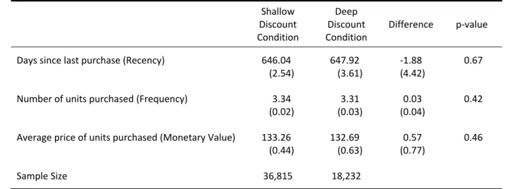
We confirm that the allocation of customers to the two conditions was random by comparing 

the historical purchases made by the two samples of customers.  In Table I we compare the 

average Recency, Frequency and Monetary Value (RFM) of customers’ purchases during the 8‐

year pre‐test period.6  If the assignment were truly random, we should not observe any 

5

 In Harrison and List’s (2004) nomenclature, this is a “natural field experiment”.  They distinguish 

between “artefactual field experiments”, which are the same as conventional lab experiments but with a 

non‐student subject pool; “framed field experiments”, which introduce field context; and “natural field 

experiments”, which also occur in a field context and use subjects who do not know that they are 

participants in an experiment.  

6 _{“Recency” is measured as the number of days since a customer’s last purchase.  “Frequency” measures} 

the number of items that customers previously purchased.  “Monetary Value” measures the average price 

(in dollars) of the items ordered by each customer.  The inter‐purchase interval (48 weeks) is much 

shorter than the average of the recency measure (646 days).  These measures are not directly 

comparable: the inter‐purchase interval describes the time between purchases, while the recency 

systematic differences in historical sales between the two samples. Reassuringly, none of the 

differences are significant despite the large sample sizes.    

Table I about here   

The Test Catalog was a regularly scheduled catalog containing 72 pages and 86 products.  The 

only differences between the two versions were the prices on the 36 “Test Items”.  These 36 

items were discounted in both versions, but the discounts were larger in the Deep Discount 

condition.  In the Shallow Discount condition, the mean discount on the Test Items was 34%. In 

the Deep Discount condition, the mean discount was 62%.  These yielded mean prices of 

$133.81 and $77.17 on the 36 Test Items in the two conditions (compared to a mean regular 

price of $203.83).  The size of the price discounts were chosen to be large enough to generate 

an effect, but not so large that they were outside the range of historical discounts (see Figure I).  

The prices of the other 50 items were all at their regular prices in both versions.     

The prices of the Test Items were presented as “Regularly $x Sale $y” in the deep discount 

version, and as “Regularly $x  Sale $z” in the shallow discount version.  The regular price ($x) 

was the same in both conditions, but the sale price was lower in the deep discount condition ($y 

< $z).  The use of identical text ensured that the discounted price was the only difference 

between the two versions, and also explains why we used shallow discounts rather than the 

regular price as a control.  There is considerable evidence that customers are sensitive to the 

word “Sale”, even when prices are held constant (Anderson and Simester 2001).  Charging the 

regular price as a control would have made it difficult to distinguish the effect of the price 

confound.  As we will discuss, using shallow discounts as a control does not affect our ability to 

measure how price adjustments affect sales.       

Mailing and Pricing Policies after the Test Catalog 

The firm agreed to use the same mailing policy for all customers once the experimental 

manipulation was over.  To confirm compliance we obtained data describing post‐test mailings 

for a random sample of 16,271 of the 55,047 customers involved in the test (approximately 30% 

of the full sample).  Customers in the deep discount condition received a mean of 48.47 catalogs 

in the post‐test period, compared to 48.77 catalogs in the shallow discount condition.  The 

difference in these means is not close to statistical significance.     

Notice also that the paper’s key finding is that sales are lower in the Deep Discount condition 

(compared to the Shallow Discount condition).  As we will discuss, the deep discounts led to an 

increase in sales from the Test Catalog itself.  If this affected the firm’s subsequent mailing 

decisions, it would tend to increase the number of catalogs mailed to customers in this 

condition.  This could not explain the decrease in post‐test sales. 

It is also useful to consider the firm’s pricing policy after the Test Catalog was mailed.  The 

distribution of discounts received in the post‐test period is reported in Figure II.  The use of 

discounts persisted, with a noticeable increase in the frequency of deep discounts.  Most 

catalogs mailed during the post‐test period contained at least some items with deep discounts.  

Because customers in the two conditions received the same downstream catalogs, this change 

in policy does not affect our ability to compare the behavior of customers in the two 

Figure II about here   

Predictions 

In Figure III we present a histogram of the number of Test Items that the 55,047 customers had 

purchased in the 8‐year pre‐test period.  Just over 47% of the customers (25,942) had not 

purchased any of the Test Items before receiving the Test Catalog.  Of the remaining customers, 

very few customers had purchased more than one or two of the 36 Test Items, with less than 

0.3% purchasing more than 10 and no customers purchasing every item.  As a result, the Test 

Catalog offered all customers an opportunity to purchase discounted Test Items that they did 

not already own.     

Figure III about here   

The opportunity to purchase discounted items from the Test Catalog provides a “strawman” 

prediction: because our measure of post‐test demand includes purchases from the Test Catalog 

itself, a standard model would predict higher demand in the Deep Discount condition (which 

offered lower prices).  We label this the “Low Prices” prediction:    

Low Prices  

Post‐test demand is higher in the Deep Discount condition than in the Shallow Discount 

Condition.   

Customer antagonism suggests an alternative prediction.  Customers in the Deep Discount 

condition were more likely to see prices in the Test Catalog that were lower than what they paid 

for the same item.  If this antagonizes customers then we might expect lower sales in this 

condition.  We label this the “antagonism” prediction:   

Antagonism  

Post‐test sales are lower in the Deep Discount condition than in the Shallow Discount 

Condition.   

This prediction requires only a relatively simple model of customer behavior.  It is sufficient that 

if customers see lower prices than what they paid then they are less likely to make additional 

purchases.  Because this is more likely to occur in the Deep Discount condition we expect fewer 

sales in that condition.7     

We will also consider three interactions.  The first interaction distinguishes the 29,105 

customers who had purchased one of the 36 Test Item before receiving the Test Catalog from 

the 25,942 customers who had not.  We only expect customers to be antagonized if they see 

lower prices on items that they had purchased.  Therefore, we expect a more negative (less 

positive) reaction to the deep discounts among the 29,105 customers with a prior purchase:8     

7

 Notice that we do not need to rule out favorable responses if customers see a higher price than what 

they previously paid.  We expect lower post‐test sales in the Deep Discount condition irrespective of 

whether there is a positive response (or no response) to seeing higher prices.  However, in Section 4 we 

do investigate how the price that customers previously paid affects their response to the deep discounts.    8 _{It is possible that customers may be concerned about whether other customers were antagonized.}  

However, previous studies have consistently reported that decision‐makers show little concern for the 

Past Purchase Interaction 

The deep discounts have a more negative impact on post‐test demand among customers 

who had previously purchased one of the Test Items.    

There is an alternative explanation for this interaction.  Because customers are unlikely to 

purchase the same item twice, customers who had already purchased may have been less likely 

to take advantage of the deep discounts in the Test Catalog.  We will investigate this explanation 

in Section 6, together with other alternative explanations.     

Customer antagonism may also depend upon how recently customers had purchased.  

Customers who purchased a long time ago may find it harder to remember the price that they 

paid.  Moreover, those who can remember the price may experience less regret about not 

waiting because they have had additional opportunities to consume.  We will investigate 

whether the time between a customer’s prior purchase and the mailing date for the Test 

Catalog contributes to the outcome:   

Time Interaction 

The deep discounts have a less negative effect on post‐test sales if the time since a 

customer’s previous purchase is longer.    

We also investigate whether there is evidence that customers who paid higher prices for Test 

Items were more antagonized by the deep discounts.  This “past price” interaction is somewhat 

complicated by the experimental design and so we will delay further discussion of it until we 

III. Initial Results

In this section we present initial findings that provide both context and motivation for the main 

analysis that follows.  To begin we ask how the deep discounts affected post‐test purchases by 

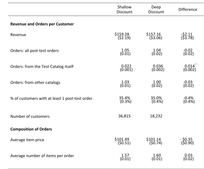
the full sample of 55,047 customers.  These results are reported in Table II, where we describe 

the average number of orders placed by customers in the Deep and Shallow Discount 

conditions.  We distinguish between orders from the Test Catalog itself, and orders from other 

catalogs (not the Test Catalog) during the post‐test period.9  We also present the average 

revenue earned, the average size of their orders and the average price of the items that 

customers purchased.     

Table II about here   

Because this overall comparison aggregates customers for whom the outcome was positive with 

others for whom it was negative, it reveals few significant differences between the two samples.  

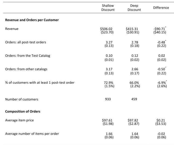
We can illustrate this by returning to the motivating example used in the Introduction.  In Table 

III we focus on customers who paid a high price (above the shallow discount price) for a Test 

Item in the 3‐months before the Test Catalog was mailed.  In the Introduction we anticipated 

that these were the customers most likely to have been antagonized by the deep discounts.       

9 _{When customers call to place an order, they are asked for a code printed on the back of the catalog.}  

This code is also printed directly on the mail‐in order form.   The data we received contain the catalog 

code for each order, so we can identify orders from the Test Catalog and orders from other catalogs.  There are a small number of orders for which the catalog code is not available, including some Internet 

orders.  Fortunately these instances are rare (there were very few Internet orders during the period of the 

Table III about here   

The deep discounts resulted in fewer post‐test orders from these customers.  In the Deep 

Discount condition customers placed an average of 2.78 post‐test orders compared to 3.27 

orders in the Shallow Discount condition.  The difference (0.48 orders or 14.8%) is statistically 

significant and can be fully attributed to the prices in the Test Catalog.  The findings also help 

clarify the source of the effect.  The differences result solely from changes in the number of 

orders placed, rather than changes in the composition of those orders; there is no difference 

between conditions in either the average number of items per order or the average prices of the 

items purchased.  The reduction in orders at least partly reflects an increase in the proportion of 

customer who placed no orders during the post‐test period (34.0% in the Deep Discount 

condition versus 27.1% in the Shallow Discount condition).  It is this result that led us to describe 

the effect as a customer “boycott”.    

The decrease in orders is a strong result: merely sending these customers a catalog containing 

lower prices reduced purchases.  The effect is large, and is precisely the outcome that managers 

appear to anticipate when stating they were reluctant to adjust prices for fear of antagonizing 

their customers (Blinder et al. 1998; Hall and Hitch 1939).  Notice that customers who had 

purchased recently (Table III) are systematically more valuable than the average customer in the 

study (Table II).  Although they place similar sized orders, the recent purchasers order a lot more 

frequently in the post‐test period.  Because they are more valuable, the cost to the firm is 

greatly amplified.  Although confidentiality restrictions prevent us from reporting detailed profit 

results, sending the deep discount version to these 1,392 customers would have lowered the 

discount version).  To put this in context, the printing and mailing cost for sending the Test 

Catalog is approximately 50‐cents, or $27,500 to send it to all 55,047 customers in the study.     

It is also helpful to remember factors that cannot explain this result.  Most importantly, the 

difference in orders cannot be explained by differences in the customers themselves.  Our 

analysis compares customers in the two experimental conditions and random assignment 

(which we verified in Table I) ensures that there are no systematic differences between 

customers in the two conditions.  We can also see that the difference in post‐test orders is not 

due to a difference in the number of orders from the Test Catalog itself.  Orders from the Test 

Catalog represent only a very small proportion (less than 3%) of overall post‐test demand.  

Moreover, orders from the Test Catalog were actually slightly higher in the Deep Discount 

condition, presumably due to the lower prices.  Finally, because our measure of sales includes 

purchases from the Test Catalog, the result cannot be explained by intertemporal demand 

substitution (forward‐buying).  Acceleration in purchases to take advantage of the Test Catalog 

discounts would not affect this measure of total orders.    

One explanation for the results, which does not depend on customer antagonism, is that the 

deep discounts may have changed customers’ expectations about the availability of future 

discounts.  If customers delayed their future purchases in anticipation of these discounts it could 

explain a reduction in post‐test sales.  As we acknowledged in the Introduction, we cannot 

completely rule out this explanation.  However, in Section 6 we will present results that suggest 

this cannot be a complete explanation for all of the findings.  In particular, if customers were 

waiting for future discounts, the decrease in post‐test sales should be larger at prices that do 

waiting for additional discounts.  However, we find that sales decrease even when the discounts 

are large.     

The initial analysis in this section focused on the sample of customers who we expected to be 

most susceptible to the antagonism prediction.  In the next section we extend the focus to all of 

the customers in the study, and measure how the effect was moderated by whether customers 

had previously purchased a Test Item and (if so) how recently they had purchased it.     

IV. The Past Purchase and Time Interactions

Because our initial analysis revealed that the primary effect is upon the number of orders 

placed, rather than the composition of those orders, we use a “count” of orders placed as the 

dependent variable (we later also use revenue and profits as dependent variables).  We 

estimate this variable using Poisson regression, which is well‐suited to count data.10  Under this 

model the number of orders from customer i (Qi) is drawn from a Poisson distribution with 

parameter λi:  

(1)  Prob

(

)

( )

! i q i i i e Q q q q −λ_λ = = λ =βX_i        

To estimate how the outcome was moderated by the time interaction since a customer’s prior 

purchase, we use the following specification: 

(2)      βXi = β1Deep Discounti+ β2Deep Discount Timei* i+β3Timei+ θZi 

These variables are defined as:  10

Deep Discounti  A binary variable indicating whether customer i was in the deep discount 

condition. 

Timei  The log of the number of months between the Test Catalog mailing date 

and customer i’s most recent purchase of a Test Item.   

For completeness the vector Z includes the log of the historical Recency, Frequency and 

Monetary Value (RFM) measures as control variables.  Because these variables do not vary 

systematically across the two conditions (Table I), their inclusion or absence has little impact on 

the coefficients of interest (β1 and β2).   Among customers who previously purchased a Test  Item, β1 describes how receiving the deep discounts affected post‐test orders by a “benchmark”  customer, who purchased a Test Item immediately before receiving the Test Catalog (Time 

equals zero).  As the time since the customer’s prior purchase increases, the estimated impact of 

the deep discounts is moderated by β2.  The time interaction predicts that β2 will have a positive  sign: the longer the time since the prior purchase, the smaller the reduction in post‐test sales.     

Notice that this model preserves the benefits of the randomized experimental design.  The 

coefficients of interest measure the percentage difference in post‐test sales between customers 

who received the deep and shallow discount versions of the Test Catalog.  As a result, the 

coefficients of interest cannot be explained by difference in customer characteristics between 

the two experimental treatments, or by intervening competitive or macroeconomic events.  We 

rely heavily on this feature of the study as it allows us to rule out a wide range of alternative 

explanations.  The model is estimated separately on the 28,642 customers who had previously 

item.11  Coefficients and standard errors for both models are reported in Table IV.     

Table IV about here   

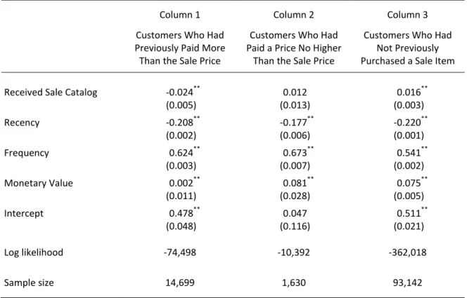
Column 1 focuses on customers with a prior Test Item purchase.  For these customers β1 is  negative and significant, indicating that for our benchmark customer (for whom Time equals 

zero) the deep discounts led to a 7.8% reduction in post‐test sales.  This replicates our univariate 

results and confirms that merely sending customers a catalog containing lower prices led to 

fewer orders by these customers.  For the same customers β2 is positive and significant.  This  result is consistent with the Time interaction, and confirms that the loss of sales is smaller when 

more time has passed since a customer’s earlier purchase.     

The findings also reveal that the drop in post‐test sales was limited to customers who had 

previously purchased one of the discounted items.  For customers who had not previously 

purchased a Test Item (Column 2) the difference in sales between the two conditions was not 

significant.   This is consistent with the Past Purchase prediction, which anticipated that the 

deep discounts would only reduce sales among customers who had previously purchased one of 

the Test Items.12   

11 _{Joint estimation of the two models yields the same pattern of results but the findings are more difficult} 

to interpret (they require three‐way interactions). For customers who had not previously purchased a Test 

Item we calculate the Time since their most recent purchase of any item.  This is the same as our Recency 

measure and so we omit Recency from this model.    12

 We did not expect these customers to be antagonized by the deep discounts, but we would have 

expected them to take advantage of the lower prices.  Further investigation confirms that when we 

We can use the coefficients in Table IV to calculate how much time is required to elapse for the 

deep discounts to have a positive effect on post‐test sales.  Given coefficients of ‐0.078 for β1  and 0.026 for β2, the net impact of the deep discounts equals zero when Time is equal to 20.1 

months.13  We conclude that the estimated impact of the deep discounts was negative if 

customers purchased a Test Item within approximately two years of receiving the Test Catalog.  

This time interaction has an important additional implication for the firm.  Recall that the initial 

findings in the previous section (and the Recency and Time coefficients in Table IV) confirm that 

customers who purchased recently are systematically more valuable ‐ they purchase 

significantly more frequently in the post‐test period.  Because the reduction in post‐test sales 

was focused on these recent customers, there was a disproportionate effect on overall sales.  

Specifically, 13,830 customers purchased a Test Item within 20.1 months of receiving the Test 

Catalog.  These customers represent just 25% of the sample but contributed approximately 52% 

of post‐test revenue.  If the firm mailed the deep discount versions (rather than shallow 

discount version) to each of these 13,830 customers its profits would decrease by approximately 

$155,000.14   

Equation (2) imposes a functional form on the interaction between the Time and Deep Discount 

variables.  We can relax this restriction by grouping customers into segments based on the time 

since their earlier Test Item purchase, and directly estimating the impact of the deep discount 

on each segment.  In particular, we group customers into four segments based on the timing of 

their earlier purchases:  less than 250 days; 250 to 500 days; 500 to 750 days; or over 750 days 

since the Test Catalog was mailed.  We then estimate the following Poisson regression model for 

13

 Calculated as  0.078 0.026

e

each segment:   

(3)  βXi= β1Deep Discounti+ θZi       

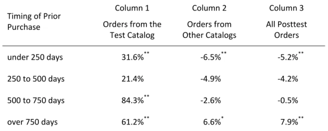
The β1 coefficients for each segment are summarized in Figure IV and complete findings are  provided in Table V.15  The deep discounts led to a significant loss of sales (‐5.22%) from the 

4,413 customers who had purchased within 250 days of receiving the Test Catalog, and a 

significant increase in sales (+7.87%) from customers whose prior purchases occurred over 750 

days ago.  The results for the other two segments fall between these two results.   This 

consistent monotonic relationship is reassuring, and confirms that we cannot attribute the role 

of time solely to the functional form imposed in Equation (2).     

Table V and Figure IV about here   

The positive outcome for customers whose prior purchases were not recent (over 750 days ago) 

is worthy of comment.   We offer two possible explanations.  First, recall that customers had 

generally purchased at most one or two of the Test Items that were discounted in the Test 

Catalog (see Figure III).  The deep discounts in the Test Catalog gave them the opportunity to 

purchase other items at low prices.  This motivated our Low Prices prediction that sales would 

be higher in the Deep Discount condition.  Second, it is possible the deep discounts persuaded 

some customers that the firm offers low prices, which may have prompted them to pay more 

attention to future catalogs (Anderson and Simester 2004).  We investigate both explanations in 

Table VI, where we distinguish orders from the Test Catalog itself and post‐test orders from 

other catalogs.     

Table VI about here 

The deep discounts led to more orders from the Test Catalog for all customer segments.  This is 

consistent with customers taking advantage of the deep discounts in that catalog to purchase 

items they had not already purchased (the Low Prices prediction).  The effect is particularly 

strong for customers whose prior purchases were less recent.  These are the same customers for 

whom we observe a positive outcome in Figure IV.  Among customers who had not purchased 

for over 750 days, the positive effect of the deep discounts extends beyond the Test Catalog to 

also increase orders from other catalogs by 6.6%.  This is consistent with our second 

explanation: more favorable price expectations may have expanded the range of occasions on 

which these customers searched for products in the firm’s catalogs.        

Summary 

We conclude that the findings offer strong support for the Past Purchase and Time interactions.  

The reduction in sales is limited to customers who had previously purchased a Test Item and is 

stronger for customers who purchased more recently.  We next consider how the price that 

customers paid in their earlier purchases influences the outcome.  We will then investigate 

whether the findings persist throughout the post‐test period, and whether they survive when 

we use post‐test measures of revenue and profit as the dependent variable.   

V. Additional Results

If price variation leads to customer antagonism, we might expect that customers who paid the 

highest prices in their earlier purchases would be most antagonized.  There is considerable 

variation in the prices that customers paid for Test Items before receiving the Test Catalog.  We 

can illustrate this variation by using this past price to group customers into three segments, 

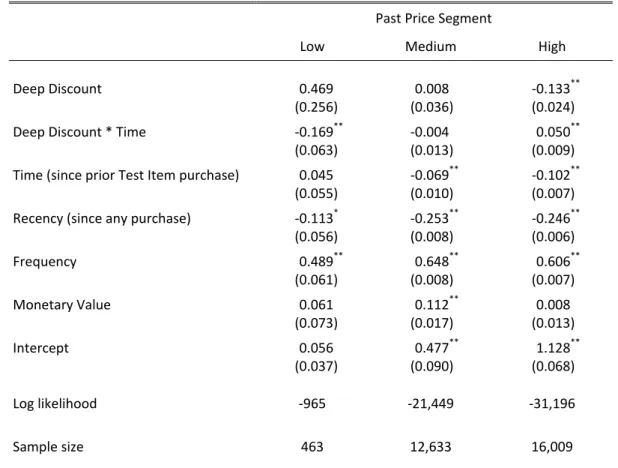
which we label “Low”, “Medium” and “High”: 

Segment  Past Price Level 

Number       

of Customers 

Low   Less than the deep discount price  463 

Medium  Between the deep and shallow discount prices  12,633 

High  Above the shallow discount price  16,009   

We do not expect the 463 customers who paid less than the deep discount price to be 

antagonized by the deep discounts.  For the 12,633 customers in the Medium segment who paid 

between the deep and shallow discount prices, the possibility of antagonism only arises in the 

Deep Discount condition, as this was the only condition where prices were lower than what 

customers previously paid.  In contrast, all of the 16,009 customers in the High segment paid 

above the shallow discount price and saw lower prices when they received the Test Catalog.  

These customers may be antagonized in both experimental conditions.   

Without knowing how customers respond to small and large price differences, we cannot make 

a clear ex‐ante prediction about how the outcome will vary across the High and Medium 

customers have the same negative reaction to any observed price reduction, then customers in 

the High segment will have the same reaction in both experimental conditions.  In contrast, 

customers in the Medium segment will react negatively in the Deep Discount condition but not 

in the Shallow Discount condition.  Our comparison of the two conditions will reveal a negative 

response in the Medium segment and no effect in the High segment.  A second (equally 

extreme) behavior is that customers only react to large price differences. It is possible that none 

of the customers in the Medium segment observe a large enough price difference to prompt a 

reaction, while the outcome in the High segment depends upon the amount customers paid.  

Customers who paid the most may react in both conditions, while others may only react in the 

Deep Discount condition. Comparison of the two conditions will reveal no effect in the Medium 

segment and a negative effect for some customers in the High segment.     

We can investigate this issue empirically.  Our experimental design ensures that within each 

segment customers were randomly assigned to the Deep and Shallow Discount conditions. 

Therefore, we can measure how the deep discounts affected post‐test sales in each segment by 

estimating Equation (3) separately for each segment.  The coefficients, which are reported in 

Table VII, reveal clear evidence that the past price plays an important role.  Customers in the 

High segment reacted adversely to the deep discounts, but we do not observe any reaction in 

the Medium segment.   Together, these results suggest that while customers react negatively to 

large price differences, they may be willing to overlook small price differences.      

Table VII about here   

These results also have an important implication for the firm.  Customers who pay higher prices 

tend to be systematically more valuable: the 16,009 customers in the High segment represent 

approximately 29% of the sample but contribute 47% of the post‐test profit.  The concentration 

of the effect amongst these customers amplifies the importance of the effect on the firm’s 

profits.        

We conclude that the reduction in demand is concentrated in the segment of customers who 

had previously paid a high price (above the shallow discount price) for a Test Item.  We will 

focus on this segment in the remainder of our analysis.   We next consider whether the findings 

persist throughout the post‐test period, and then investigate whether they survive when we use 

post‐test measures of revenue and profit as the dependent variable. 

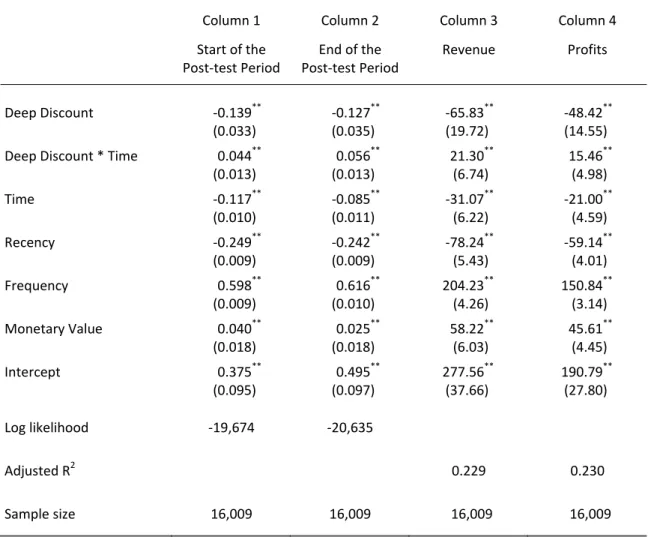
Does the Adverse Outcome Persist? 

To evaluate the persistence of the results we divided the 28‐month post‐test period into two 

fourteen‐month sub‐periods.  We estimate Equation (2) on both sub‐periods and report the 

findings in Table VIII (Columns 1 and 2).  Comparing β1 and β2 between the two data periods  reveals no significant difference in either coefficient (they are also not significantly different 

from the findings reported for these customers in Table VII).  However, the results do imply a 

different time cutoff for which there is a negative response to the deep discounts.  At the start 

of the post‐test period the negative response extends to customers who purchased within 23.5 

months of receiving the Test Catalog.  At the end of the period the results indicate that the 

response is only negative for customers whose prior purchase occurred with 9.7 months of the 

Test Catalog.  We conclude that although the negative effect survives for more than a year after 

Profit and Revenue 

The regression results reported so far consider only the number of orders purchased during the 

post‐test period.  To evaluate robustness we also analyzed two additional dependent measures: 

the Total Revenue and Total Profit earned from each customer during the post‐test period 

(where profit is calculated as revenue minus cost of goods sold).  Both variables are continuous 

rather than count measures and so we estimate the models using OLS.  The findings are 

reported in Table VIII (Columns 3 and 4).  They confirm that deep discounts lead to a reduction 

in both revenue and profits.  This effect diminishes as the time since a customer’s previous 

purchase increases.  The interval at which the net effect is zero is approximately 22 months for 

both metrics.   

Table VIII about here   

Summary 

We conclude that lower prices leads to fewer purchases by some customers.  This effect is 

strongest amongst customers who had recently paid a high price to buy an item on which the 

price is later lowered.  Unfortunately these include many of the firm’s most valuable customers, 

magnifying the importance of the effect.  Readers who are solely interested in the existence of 

this effect may want to read ahead to Section 7, where we replicate the findings with a different 

company in a different product category.  However, other readers may be interested in 

reviewing alternative explanations for these outcomes.  We address this issue in the next 

VI. Alternative Explanations

The findings reported in the previous sections are consistent with customer antagonism.  In this 

section we evaluate three alternative explanations for the findings.  We begin by considering the 

possibility that customers delayed their purchases in anticipation of future discounts.  We then 

consider the role of both quality signals and demand depletion.     

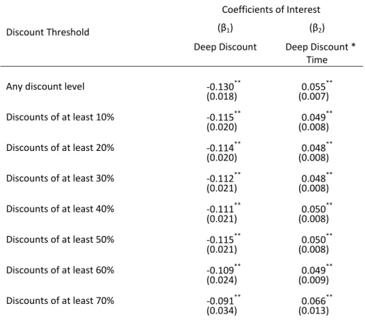
Delayed Purchases 

Coase recognized that customers may respond to inter‐temporal discounts by delaying their 

purchases in anticipation of future discounts (Coase 1972).  In our context, the discounts in the 

Deep Discount condition may have alerted customers to the possibility of future discounts.  If 

customers responded by delaying their subsequent purchases, this might explain the reduction 

in post‐test orders.  As we have already acknowledged, we cannot fully rule out this explanation, 

but we can investigate it using several approaches.      

First, if customers were waiting for future discounts, the decrease in post‐test sales should be 

larger at prices that represent either small discounts or no discounts.  It is these purchases that 

we would expect customers to forgo while waiting for larger discounts.  To investigate this 

prediction we re‐calculate post‐test sales using different discount thresholds.   For example, 

“Discounts of at least 60%” counts the number of units in the post‐test period at discounts of at 

least 60%.16  We re‐estimated Equation (2) using eight different discount thresholds and report 

the results from each of these eight models in Table IX.        

Table IX about here   

Though not statistically significant, there is weak evidence of a trend in the results.  At higher 

discount thresholds the Deep Discount coefficients are slightly less negative, which is consistent 

with customers waiting for larger discounts.  Moreover, the implied Time at which the effect 

switches from negative to positive becomes shorter (indicating that we only observe a negative 

effect among customers who purchased immediately before receiving the Test Catalog).    

However, the findings also confirm that sales decrease even for deeply discounted items, which 

is difficult to reconcile with customers waiting for future discounts.       

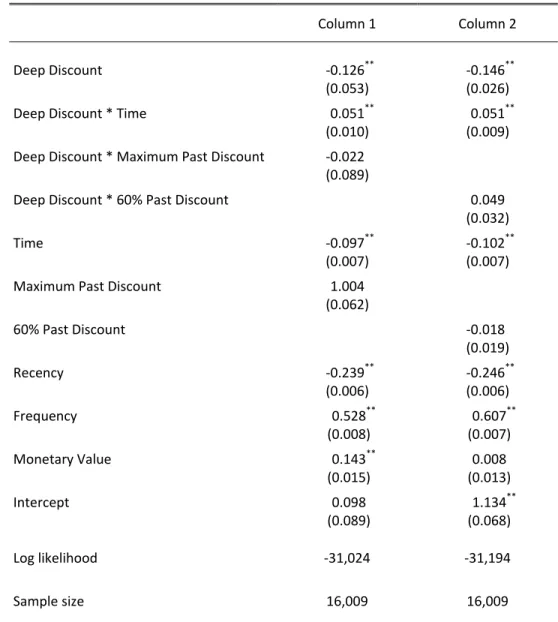
Our second approach recognizes that deeply discounted prices were not unique to the Test 

Catalog.  Over 38% of purchases in the pre‐test period were made at discount levels of at least 

50% (see Figure I).17  If customers had purchased at deep discounts in the past, it seems less 

likely they would be surprised by the deep discounts in the Test Catalog, or that they would 

change their behavior by delaying future purchases.  Therefore, we can evaluate this alternative 

explanation by investigating whether the decrease in demand was smaller among customers 

who had purchased at deep discounts in the pre‐test period.  We do so by including a measure 

of past discounts in our model:   

(4)      β     1 2 3 4 5 * * Z i i i i i i i i i

Deep Discount Deep Discount Time Time

Deep Discount Maximum Past Discount Maximum Past Discount

= β +β +β

+β +β + θ

X

17 _{Many pre‐test purchases were made at even deeper discounts (14.6% were made at a discount of at} 

least 60%).  Recall that we used a 60% discount level in the Deep Discount condition because it was 

where Maximum Past Discounti measures the largest percentage discount on any item that 

customer i purchased during the pre‐test period.  We report the coefficients for this model in 

Table X.  We also include an alternative model in which Maximum Past Discounti is replaced with 

a binary variable (60% Past Discounti) identifying customers who had previously purchased at a 

discount of at least 60%.     

Table X about here   

Neither of these interaction terms approaches statistical significance.  The response to the deep 

discounts was apparently not affected by the size of the discounts that customers had received 

in the past.  This is not what we would expect if the Test Catalog changed customers’ price 

expectations; the effect should be strongest for customers who had not previously purchased at 

a large discount.      

We make a final observation about this explanation.  At the start of Section 3 we reported the 

average price of the items purchased in the post‐test period (Table III).  Increased willingness to 

wait for discounts should lead to customers paying lower average prices.  However, the average 

price paid (per unit) was not significantly different between the two conditions.     

We conclude that delay in anticipation of future discounts does not appear to be a complete 

explanation for the results.     

Quality Signals 

It is possible that customers interpreted the deep discounts on the Test Items as a signal that 

these items were of inferior quality.  To investigate this possibility, we can restrict attention to 

non‐Test Items (“other items”).  We do not expect discounts on the Test Items to signal 

information about the quality of these other items, and so if the effect persists for these other 

items, it is unlikely to be due to an adverse quality signal.    

The Test Items accounted for only 22% of the 94,487 post‐test purchases, so the remaining 78% 

of the purchases were for the approximately 400 other items sold by the firm.  We repeat our 

earlier analysis when distinguishing between post‐test sales for Test Items and other items and 

report the results in Table XI.  The pattern of findings is unchanged.  Indeed, the findings are 

stronger for these other items than for the Test Items, presumably because some customers 

took advantage of the deep discounts (on the Test Items) in the Test Catalog.  We conclude that 

the decrease in sales cannot be fully explained by customers using the deep discounts as a signal 

that the Test Items are poor quality.     

Table XI about here   

An alternative interpretation is that the deep discounts lowered the perceived quality of all of 

the products sold by the firm.  This is a relatively implausible explanation in this setting.  Most 

customers in the study had made multiple previous purchases and had received a large number 

of catalogs from the firm.  On average, each customer had purchased approximately 3.3 units 

prior to receiving the Test Catalog.  This increases to 5.2 units among customers who had