Mathematics Faculty Publications and Presentations Department of Mathematics
11-1-2018
Efficient Blind Image Deblurring Using
Nonparametric Regression and Local Pixel
Clustering
Yicheng Kang
Bentley University
Partha Sarathi Mukherjee
Boise State University
Peihua Qiu
University of Florida
Efficient
Blind
Image
Deblurring
Using
Nonparametric
Regression
And
Local
Pixel
Clustering
Yicheng
Kang
Department
of
Mathematical
Sciences,
Bentley
University
Partha
Sarathi
Mukherjee
Department
of
Mathematics,
Boise
State
University
and
Peihua
Qiu
Department
of
Biostatistics,
University
of
Florida
November
27,
2017
Abstract
Blindimagedeblurringisachallengingill-posedproblem. Itwouldhaveaninfinite
number of solutions even in cases when an observed image contains no noise. In
reality,however,observedimages almostalwayscontain noise. Thepresenceof noise
would make the image deblurringproblem even more challenging because the noise
cancausenumericalinstabilityinmanyexistingimagedeblurringprocedures. Inthis
paper, a novelblind imagedeblurringapproach is proposed,which canremove both
pointwise noiseand spatial blur efficiently without imposing restrictive assumptions
on eitherthepoint spreadfunction(psf)orthetrue image. It evenallows thepsfto
be locationdependent. In theproposed approach,a local pixel clustering procedure
is used to handle the challengingtask of restoring complicated edge structures that
are tapered by blur,and a nonparametric regression procedureis usedfor removing
noise at the same time. Numerical examples show that our proposed method can
effectively handlea widevarietyof blurand it workswellinapplications.
Keywords: Blind image deblurring; Clustering; Deconvolution; Denoising; Edges; Image reconstruction; Smoothing; Surfaceestimation; Nonparametric regression.
1
Introduction
Observed images are not always faithful representations of the scenes that we see. As a matter of fact, some sort of degradation often arises when recording a digital image. For instance, in astronomicalimaging, the incoming lightin the telescope is often bent by at mospheric turbulence. In aerial reconnaissance, the optical system in camera lens could be out of focus. In our daily life, image distortion often arises in cases when there is a relative motion between a camera and an object. Environmental effects such as scattered and reflected lightalsodegradeimages. Other sourcesofdegradationsincludedevice noise (e.g., charge-coupled device sensor and circuitry) and quantization noise. See Bates and McDonnell (1989) and Gonzalez and Woods (2008)for a detailed discussion about forma tion and description of various degradations. Classically, image degradation is modeled as the result of two phenomena (Aubert and Kornprobst, 2006). The first one is related to the image acquisition (e.g., blur created by motion). The second one is random and corresponds tothe noise comingfrom signal transmission.
In the literature, a commonly used model for describing the relationship between the true image f and itsdegraded version Z is asfollows.
Z(x,y) = G{f}(x,y) +ε(x,y), for (x,y)∈Ω, (1)
whereG{f}(x,y) = R2g(u,v;x,y)f(x−u,y−v)dudv denotesthe convolutionbetween
a 2-D point spread function (psf) g and a true image intensity function f, ε(x,y) is the pointwisenoiseat(x,y),andΩisthedesignspaceoftheimage. Inmodel(1), itisassumed that the true image f is degraded spatially by g and pointwise by ε, the spatial blur is linear, and the pointwise noise is additive. In most references, it is further assumed that thepsfg,whichdescribestheblurringmechanism,islocation(orspatially)invariant. That is, g(u,v;x,y)does not depend on(x,y).
Blindimagedeblurring(BID)isforestimatingffromZwhenthepsfgisnotcompletely specified. This problem is ill-posed in nature because only Z is observed in (1), all g, f
and ε are unobservable, and it is impossible to distinguish (g,f) from (ag,a−1f) based
on the observed image Z alone, for any constant a = 0. This ill-posed nature would get even worseincaseswheng changesoverlocation. Inthe literature,some imagedeblurring
procedureshavebeendevelopedunder the assumptionthat thepsf g is completelyknown. Suchproceduresare oftenreferredtobe non-blind. The maindifficulty innon-blindimage deblurring liesbehind the removalof blurinpresence of noise(cf.,Qiu (2005),Chapter 7). To overcome this difficulty, a number of image deblurring techniques have been proposed using the regularization framework (e.g., Chan and Wong (1998), Figueiredo and Nowak (2003), Oliveira et al. (2009), Rudin et al. (1992), You and Kaveh (1996)). In practice, however,itishardtospecifythepsfgcompletely. Incaseswhentheassumedpsfisdifferent from the truepsf, ithas been shown thatthe deblurred image couldbe seriously distorted (cf., Qiu (2005), Chapter 7). To avoid such limitations, a number of BID methods have been developedin the literature. Some of them assume that g followsa parametric model with one or more unknown parameters,and these parametersare estimated together with the trueimage f bycertainalgorithms (e.g.,Carasso(2001),Carasso(2003),Halland Qiu (2007b), Joshi and Chaudhuri (2005), Katsaggelos and Lay (1990)). Some others assume that the true image f has one or more regions with certain known edge structures or the image’sedgestructurescanbeestimatedreasonablywell(e.g.,HallandQiu (2007a),Kang and Qiu (2014), Kundurand Hatzinakos (1998), Qiu (2008), Qiu and Kang (2015), Yang et al. (1994)). Some BID methods adopt the Bayesian framework to make the originally ill-posed BID problem well-posedbyimposing someprior information onthe psfor onthe true image (e.g., Fergus et al. (2006), Miskin and MacKay (2000), Skilling (1989)). Some other BID methods estimate both g and f in an alternating fashion, using the iterative Richardson-Lucy scheme (e.g.,Biggs and Andrews (1997), Jansson(1997)).
This paper proposes an alternative approach to the BID problem based on the obser vation that spatial blur alters theimage structure most dramatically around step edges and least dramatically at places where the true image intensity surface is straight. Based on this observation, our proposed approach focuses on deblurring around step edges. More specifically, it works as follows. In a neighborhood of a given pixel, if we conclude based on a data-driven criterion that there could be step edges in the neighborhood, then all pixels are clustered into two groups. In such cases, the image intensity atthe given pixel is estimated by a weighted average of all image intensities in the group that the given pixel belongs to. If we conclude that there are no step edges in the neighborhood, then
� � �
the image intensity at the given pixel is estimated by a weighted average of all image in tensities in the entire neighborhood. One major feature of this approach is that it does not require any restrictive assumptions on either g or f. It even allows g to vary over location. Numerical comparisons with some representatives of the state-of-the-art image deblurringmethodsshowthattheproposedmethodiscapableofhandlingawidevarietyof blur and it works wellin various applications. The proposed method can be accomplished by the functions surfaceCluster() and surfaceCluster bandwidth() in the R-package DRIP
(https://cran.r-project.org/web/packages/DRIP/). The test images used in Section 3 are also included inthe package.
The rest part of the paper is organized as follows. Our proposed methodology is de scribedindetailinSection2. SomenumericalexamplesarepresentedinSection3. Several remarks conclude the paper inSection 4.
2
Methodology
We describeour proposedBID methodintwo parts. InSubsection 2.1,our new methodis described indetail. In Subsection 2.2, selection of procedure parameters isdiscussed.
2.1
Proposed
BID
Method
Assume that an observed image followsthe discretized versionof model (1)
Zij =G{f}(i,j) +εij, for i,j = 1,2,...,n,
where(i,j)denotethe (i,j)-thequallyspacedpixel(i.e., thepixellocatedat(i/n,j/n))in the design space Ω = [0,1]×[0,1], {Zij,i,j = 1,2, . . . , n} are observed image intensities,
and {εij,i,j = 1,2, . . . , n} are independent and identically distributed (i.i.d.) random
errors with mean 0 and unknown variance σ2. It is further assumed that f is continuous
in Ω except on some edge curves (see Qiu (1998) for a mathematical definition of edge curves).
Forthe (x,y)-th pixel, letus consideritscircular neighborhood
where the positive integer k ≤ n is a bandwidth parameter and (x,y) denotes the two-dimensionalindex ofthedesignpoint(wewill alsorefertothe pixeloritslocationas(x,y) and its meaning should be noambiguity fromthe context ). Inthis neighborhood, a local planeisfittedbythefollowinglocallinearkernel(LLK)smoothingprocedure(cf.,Fanand Gijbels (1996)): � n n 2 � t t b c i−x j−y min Zij −a− (i−x)− (j−y) K , , a,b,c n n k k i=1 j=1 (2)
whereK isacircularlysymmetricbivariatedensitykernelfunctionwith itssupportonthe unit disk. The aboveLLK smoothing procedureapproximates the image intensity surface locallybyaplaneandusesthekernelfunctionK tocontroltheweightsintheweightedleast squares procedure (2). Usually, K is chosen such that pixels closer to (x,y) receive more weights, which isintuitively reasonable because pixelscloserto (x,y)should providemore information about the image intensity at(x,y). Let (ban(x,y),bbn(x,y),bcn(x,y))denote the
solutiontotheminimization problem(2). Themathematical expressionsare shownin(12) - (14)in the appendix. Then, ban(x,y) in(12) isthe LLKestimator of f(x,y), andbbn(x,y)
and bcn(x,y) are the LLK estimators of the x and y derivatives of f at(x,y), respectively,
in cases when suchderivatives exist.
The LLK estimator removes noise but also blurs edges at the same time. Center weighted median (CWM) filtering is a useful method in image processing and it can pre serve edges tosome extent (Ko and Lee, 1991;Sun et al., 1994). Next, a CWMfilter with center weight W0,0 is applied to O(x,y;k,n) and the filter output at (x,y) is denoted by
a
˜n(x,y). The residual at(x,y) is definedby
en(x,y) =ban(x,y)−a˜n(x,y). (3)
If(x,y)isinthecontinuityregionoff,thentheimagestructurewithinO(x,y;k,n)should
b
be approximated well by the local plane described by (ban(x,y), bn(x,y),bcn(x,y)). Thus,
en(x,y)shouldberelativelysmall. Onthe otherhand,ifO(x,y;k,n)containsedgecurves,
then the fitted local plane cannot well describe the image structure within O(x,y;k,n). Consequently, the value of e(x,y) should be relatively large. Therefore, en(x,y) can be
specifically, if
|en(x,y)|> un, (4)
then we can conclude that there are edge curves in O(x,y;k,n), where un is a threshold
value. In such a case, we can cluster the pixels in O(x,y;k,n) into two groups based on their CWM outputs. Intuitively, pixels on the same side of an edge curve have similar CWMoutputs. So, theycan beputinthesamegroup. Pixelsondifferentsidesof theedge curve have quite different CWM outputs, and they should be put in different groups. Of course,itisnoteasytospecifythe exactpositionof theedgecurvewithinO(x,y;k,n)and define the two groupsof pixels accordingly. But, aninformative pixelclustering procedure can generate groups such that pixels within a group are similar in their CWM outputs and pixels in different groups have quite different CWM outputs. Such a pixel clustering procedure can reflect the local edge structure wellwithout imposing restrictive conditions on the smoothness or shape of the edge curve. In this paper, we suggest a simple but effectivepixelclusteringprocedurewhichusesacut-offconstantctodefinethetwoclusters in O(x,y;k,n). Morespecifically, the two clusters are definedto be
O1(x,y;k,n,c) = {(i,j)∈O(x,y;k,n) : ˜an(i,j)≤c},
O2(x,y;k,n,c) = {(i,j)∈O(x,y;k,n) : ˜an(i,j)> c},
where c ∈ R(x,y;k,n), and R(x,y;k,n) is the range of the image intensity values in
O(x,y;k,n) definedto be
R(x,y;k,n)= min a˜n(i,j), max a˜n(i,j) .
O(x,y;k,n) O(x,y;k,n)
So, it is obvious that both O1(x,y;k,n,c) and O2(x,y;k,n,c) are non-empty sets for
any constant c ∈ R(x,y;k,n), O(x,y;k,n,c) = O1(x,y;k,n,c) ∪ O2(x,y;k,n,c), and
O1(x,y;k,n,c) ∩O2(x,y;k,n,c) = ∅. Let c0 be the maximizer to the following maxi
mization problem: (5) |O1(x,y;k,n,c)|(η1−η)2+|O2(x,y;k,n,c)|(η2−η)2 max t t , c∈R(x,y;k,n) (˜a n(i,j)−η1) 2 + (˜an(i,j)−η2) 2 O1(x,y;k,n,c) O2(x,y;hn,c)
where |A| denotesthe number of elements inthe pointset A, ηs denotes the sample mean of the CWM outputs within Os(x,y;k,n,c), for s = 1,2, and η denotes the sample mean
� �
of the CWMoutputswithinO(x,y;k,n). In (5), the numeratormeasuresthe dissimilarity between the two groups, and the denominator measures the dissimilarity within each of the twogroups. Thus,itisreasonabletoclusterthe pixelsinO(x,y;k,n,c)bymaximizing their ratio. It can be checked that (5) is actually the one dimensional version of the well-known clustering criterion proposed by Friedman and Rubin (1967). Note that there are only finitely many cut-off constants that can result in different partitions. Namely, it is sufficient toevaluate(5) onthe finitesetof {a˜n(i,j) : (i,j)∈O(x,y;k,n)}. Therefore,the
maximization problem can besolved by exhaustivesearch.
Without loss of generality, assume that (x,y) ∈ O1(x,y;k,n,c0). Then, a weighted
average ofobservationsinO1(x,y;k,n,c0)shouldprovideagoodestimate forf(x,y)when
there isnoblurringinvolved, asdiscussedinthe imagedenoising literature(cf., Qiu1998). In cases when the observed image contains blur, if the intensity value of a pixel is closer to the cut-off constant c0, then it should receive less weight in the weighted average since
it is more likely that that pixel has blur involved. To address this issue related to the image blur, besides a bivariate kernel function used in the conventional kernel smoothing procedure to assign more weights to pixels closer to(x,y), a univariate kernel function is used to assign less weights to pixels whose intensity values are closer to c0. Then, our
proposed BID estimator fbn(x,y) is defined to be the solution to a0 in the following local
constant kernel (LCK) smoothingprocedure:
(6) t 2 i−x j−y |˜an(i,j)−c0| min (Zij −a0) K , L (1) , a0∈R k k |˜ −c 0| O1(x,y;k,n,c0) amin (1)
where Lis aunivariateincreasing densitykernel functionwith the support[0,1],and ˜amin
b
denotes the minimum CWM output in O1(x,y;k,n,c0). It is easy to check that fn(x,y)
has the following expression:
i−x j−y |a˜n(i,j)−c0| , L O1(x,y;k,n,c0)ZijK k k |a˜(1) −c0| b min fn(x,y) = . i−x j−y |˜an(i,j)−c0| O1(x,y;hn,c0)K k , k L |˜a(1) −c0| min (7) b
In cases when (x,y) ∈ O2(x,y;k,n,c0), fn(x,y) can be defined in the same way except
(1) (2)
that O1(x,y; k,n,c0) and ˜amin in (7) should be replaced by O2(x,y;k,n,c0) and ˜amax,
(2)
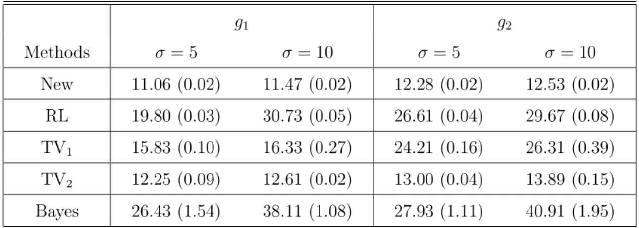
Todemonstratetheefficacyof theimagedeblurring procedure(7), acrosssectionof an imagearoundastepedge,ablurredversion,ablurred-and-noisyversion,andthedeblurred version by (7) when K and L are chosen to be the ones used in Section 3 are shown in plots (a)-(d) of Figure 1, respectively. From plot (d), it can be seen that (7) can restore the blurrededge structure to some extentwhile removing the noise at the same time.
Figure 1: (a): A cross section of an image intensity surface around a step edge; (b): A blurred version of (a); (c): A blurred-and-noisy version of (a); (d): The deblurred version from (c) bythe BID procedure(7).
In cases when (4) is not satisfied, it is likely that the pixel (x,y) is in a continuity region of f. In such cases, the spatial blur would not alter the image intensity surface much, as discussed in Section 1. So, we suggest estimating f(x,y) by the conventional LLK estimator ban(x,y) defined in(12). There are two benefits of doing this. First, it has
been well demonstrated in the literature that the LLK estimator has less bias compared to the LCK estimator in continuity regions of f (cf., Fan and Gijbels (1996)). Second,
sinceban(x,y)hasalready beencomputedbeforewecompute fbn(x,y)in(10), itsavesmuch
computation.
2.2
Parameter
Selection
In the proposed BID procedure(5)–(7), there are two parameters tochoose, including the threshold value un in (4) and the bandwidth parameter k in (2). To choose a reasonable
valueforun,weneedtoderivetheasymptotic distributionofen(x,y)definedin(3). Based
on (3), we havethe following proposition.
Proposition 1. Let Ψ(·) and ψ(·) denote the cumulative distribution function (cdf ) and
the probability density function of ε11, respectively. Under the regularity conditions (B1) – (B5) in Appendix B and assume that(x,y) is a continuity point, then
⎡⎛ ⎞⎤ ⎞⎞ k⎣⎝ ban(x,y) ⎠−⎝ G{f}(x,y) ⎠⎦ d →N⎝⎝ 0 ⎠,⎝ Σ11 Σ12 ⎠⎠, ˜ an(x,y) G{f}(x,y) 0 Σ21 Σ22 ⎞ ⎛ ⎛⎛ ⎞ ⎛ where � � Σ11=σ2 K(x,y)2 dxdy, x2+y2≤1 E|ε11| Σ12= Σ21= , 2πψ(0) 1 Σ22= , 4πψ(0)2 d
and → denotes convergence in distribution as n→ ∞.
The proofof Proposition1 isprovided in AppendixB. If (x,y) is acontinuity point,it follows fromProposition 1that
d
k(ban(x,y)−a˜n(x,y))→N(0,Σ11+ Σ22−2Σ12).
So areasonable choice for the threshold in(4) would be
un=Z1−α/2(Σ11+ Σ22−2Σ12)/k, (8)
where Z1−α/2 denotes the 1−α/2 percentile of the standard normal distribution and α
E|ε11|,tobeestimated. We suggestapplyingasurface estimator(e.g., Qiu2009)toobtain residuals {εb11,· · · , εbnn}. Then ψ(0), σ 2,and E|ε 11| can be estimated by (9) t t t 1 εbij−0 1 1 n , σb2 = n b -n |b ψ(0)= K1 2 εij 2, E|ε 11|= 2 εij|, n2h
ni,j=1 hn n i,j=1 n i,j=1
whereK1(·)istheone-dimensionalGaussiankernelandhn= 1.06bσn
−2/5 (Wandand Jones
1994, Chapter 2).
Next,wediscussthe selectionof thebandwidthparameterk. Innumericalsimulations, the true imageis oftenknown. In suchcases, k can be chosen by minimizing
(10) t 2 MSE(f,fb;k) = 1 2 n f(i,j)−fbn(i,j) , n i,j=1
wherefbnisthedeblurredimage. Inpractice,f isusuallyunknown. Insuchcases, thecross
validation (CV) approach is natural to consider (cf., Qiu 2005, Chapter 2). In the image deblurring problem, however, the mean response is G{f}, instead of f. In such cases, the CV approach is inappropriate to use because the chosen parameter is for approximating
G{f}. To overcome this limitation of the conventional CV approach, we propose the following modified cross validation (MCV)approach.
(11)
t 2 t 2
w 1−w
MCV(k) = |Ω\J| Zij −fb−Zij(i,j) + |J| Z˜ij −fb−Z˜ij(i,j) ,
Ω\J J
wherew∈[0,1]isaconstant,J ={(i,j) :|en(i,j)|> un},fb−Zij(x,y)denotestheproposed
the BIDestimate at(x,y)withthe observationZij heldout, andZ˜ij isthe imageintensity
(1) (2)
whoseCWMoutputequalto˜amin in(7)ora˜max in(7)’salternativeforminthe caseswhen (i,j) ∈ O2(i,j;k,n,c0). The rationale behind (11) is again based on our key observation
that spatial blur alters image most dramatically around step edges and least dramatically atplaceswherethetrueimageintensitysurfaceisstraight. Morespecifically,theintensities of the pixels in the continuity region are not altered much by blur. Thus the first term in (11) uses the conventional leave-one-out CV approach. As for the pixels around step edges, their observed image intensities are no longer representative of f. We approximate them with a nearby pixel’s image intensity that is not affected dramatically by blur (i.e.,
Z˜ij in the second term of (11)). MCV is a weighted average of the two and w represents
By taking into account all these considerations, our proposed BID procedure is sum marized below.
Proposed Blind Image Deblurring Procedure
1. Foragiven pixel(x,y),solve theminimization problem (2) and computeits solution by (12)-(14).
2. Apply CWM filterand obtain˜an(x,y)
3. Compute the residualen(x,y) in (3).
4. If(4) holds, then executethe localclustering procedurebysolving the maximization problem (5), and estimate f(x,y)by (7). Otherwise, estimate f(x,y) by(12).
3
Numerical
Study
In this section, we discuss several numerical examples concerning the performance of the proposed BID procedure and the MCV bandwidth selection procedure. Throughout this section,thecenterweightW0,0intheCWMfilterischosentobe3,thesignificancelevelαis
chosen tobe0.001,therelativeweightin(11)is0.5,thetwo dimensionalkernelfunctionK
usedin(2) and(7)ischosentobe(2/π)(1−x2−y2)I(x2+y2 ≤1),andtheonedimensional
kernel function L used in (7) is chosen to be (1/1.194958)exp(x2/2)I(0 ≤ x ≤ 1). We choose these two kernelfunctions because the former is the Epanechnikov kernelfunction, whichisastandardchoiceinthestatisticalliterature,andthelatterisatruncatedGaussian kernel function, which iscommonly used inthe computer scienceliterature.
3.1
Numerical
Experiment
with
Lena
Image
We denote the proposedBID procedureas NEW and compare itwith threeother popular methods. The first existing method considered here isthe one accomplishedby the MAT LAB blind deconvolution routine deconvblind, which is based onthe method discussed by Biggs and Andrews (1997) and Jansson (1997) under the framework of Richardson-Lucy (RL) algorithm. The secondexisting method is the total variation (TV)image deblurring
method proposed by Oliveira et al. (2009). The third existing method is the blind image deconvolution proceduredevelopedunder the Bayesianframework byFergus etal.(2006). These three existing methods are denoted as RL, TV and Bayes, respectively. It should be pointed out that both RL and Bayes are blind image deblurring schemes, but TV is designed for non-blind image deblurring. Two versions of TV, denoted as TV1 and TV2,
distinguishedbyhow thepsf g isspecified,are considered. Thespecific description ofTV1
and TV2 will be given later. The bandwidth k used in (2) is chosen by minimizing(10).
The Lena test image has 512×512 pixels. The following two psf’s are considered:
⎧ g1(u,v;x,y) = g2(u,v;x,y) = ⎪ ⎨ ⎪ ⎩ ⎧ ⎪ ⎨ ⎪ ⎩ 1 exp{−u2+v2 2 +v }I(u 2 ≤0.012) if y >0.5, C1(x,y) 2 δ0(u)δ0(v) otherwise; 1 I(|u| ≤0.01)δ 0(v) if |x−0.5| ≤0.3 and |y−0.5| ≤0.3, C2(x,y) 1 δ 0(u)I(|v| ≤0.1) otherwise, C2(x,y)
where Cj(x,y) is the standardization constant such that R2gj(u,v;x,y) dudv = 1, for
any (x,y)∈Ω and j = 1,2, and δ0(·) is the delta function with the point mass at0. The
random noise is generated from the normal distribution N(0, σ2), and two different noise
levels σ = 5 and 10 are considered. From the above expression, we can see that g1 is a
truncated Gaussian blur for the upper half of the image and there is noblur for the lower half;g2isahorizontalmotionblurforthe centralpartoftheimageandisaverticalmotion
blurfortherestpartoftheimage. Inthecasewhenpsfisg1,TV1 andTV2 denotestheTV
method whenthe psf isspecifiedasthe Gaussianblur of g1 and the delta function(i.e., no
blur) of g1, respectively. In the case when psfis g2, TV1 and TV2 denotesthe TVmethod
when the psf is specified as the horizontal motion blur of g2 and the vertical motion blur
of g2, respectively.
Figure 2(a)-(c) present the original Lena image, its blurred version with g2, and its
blurred-and-noisy version with g2 and σ = 10, respectively. Figure 2(d)–(h) present the
deblurred images by NEW, RL, TV1, TV2 and Bayes, respectively. It should be pointed
out that the support of the psf needs tobe specified when using RL and the true support of g2 is used inthis exampleto showitsbest performance,and a subregion definedby the
�
inFergusetal.(2006)thattheiralgorithmwouldperformbetter andrunfasterifasmaller patch, rich in edge structure, is manually selected. From Figure 2, it can be seen that (i) NEW removesnoise and the blurwell, (ii)there are manyartifacts inthe deblurredimage of RL and the noise has not beenreduced much, and (iii) TV generates manyartifacts at places where the psf is misspecified.
Figure 2: (a)–(c): Original Lena image, its blurred version and its blurred-and-noisy ver sion, respectively. The RMSE of (c) and (d) is 15.12 and 12.51, respectively. (d)–(h): Deblurred images byNEW, RL,TV1, TV2 and Bayes, respectively.
Next, we compare the five methods quantitatively. Table 1 presents the values of the root mean squared error (RMSE) defined to be RMSE= ni,j=1[f(i,j)−fbn(i,j)]2/n2 of
the fivemethodsforeachcaseconsideredbasedon100replicatedsimulations. Thenumber in eachparenthesisrepresentsthe standard errorof the corresponding RMSE.From Table 1, itcan beseen that NEW outperformsall the other fourmethods.
� �
Table 1: Estimated values of RMSE of the five image deblurring methods in the Lena image example based on 100 replicated simulations. The numbers in the parentheses are the standard errors of RMSE.
Methods g1 σ=5 σ=10 g2 σ=5 σ=10 New 11.06 (0.02) 11.47 (0.02) 12.28 (0.02) 12.53 (0.02) RL 19.80 (0.03) 30.73 (0.05) 26.61 (0.04) 29.67 (0.08) TV1 15.83 (0.10) 16.33 (0.27) 24.21 (0.16) 26.31 (0.39) TV2 12.25 (0.09) 12.61 (0.02) 13.00 (0.04) 13.89 (0.15) Bayes 26.43 (1.54) 38.11 (1.08) 27.93 (1.11) 40.91 (1.95)
3.2
Numerical
Experiment
with
Peppers
Image
Next, we discuss the second numerical example, in which the test image of peppers with 256×256 pixelsis used. The psf g consideredhas the expression:
g(u,v;x,y)= 3 πr2(x,y) 1− u2 r2(x,y)+ v2 r2(x,y) I(u 2 +v2 ≤r2(x,y)),
where r(x,y)>0 may change over location and it is the radius of the circular support of
g. In this paper, r(x,y) is called the blur extent function. Three blur extent functions,
r1(x,y) = 0.03(1−(x−0.5)2−(y−0.5)2), r2(x,y) = 0.03x, r3(x,y) = 0.02, and two noise
levels, σ = 5, σ = 10, are considered. Clearly, r1(x,y) and r2(x,y), are location variant.,
andr3(x,y)islocationinvariant. Inthecasewithr3(x,y),theblurdescribedbyg(u,v;x,y)
ishomogeneousacrossthe entire image,which isthecase discussedbymost references. As in the previous example, the noise is generated fromthe distribution N(0, σ2). Regarding
the four image deblurring methods, we would like to make the following remarks. (i) RL requires the blur extent function to be constant (i.e., location invariant) and completely specified. So, in this example, we searched the value of r toachieve the minimum RMSE such that RL performs the best. (ii) TV requires the psf g to be completely specified and the blur extent function needs to be constant as well. In this example the value of
�
form of g is correctly specified. (iii) The prespecified subregion for Bayes is chosen to be [78/256,206/256]×[42/256,170/256].
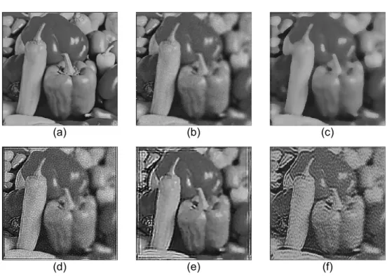
Theresults inthe same setup asFigure2are shown in Figure3,wherethe blur extent function r2(x,y) and σ = 10 are considered. From the figure, it can be seen that (i)
the blur gets more severe when moving from the left side of the image to the right side (cf., plot(b)), (ii) NEW deblurs the image and removes the noise well, (iii) RL performs poorly, (iv) the middle part of the deblurred image by TVlooks good but the places near the boundary contain many artifacts because TVcannot handle location variantblur, (v) Bayes performs poorlyinthis example. It isworthnoting thatthe RMSEofthe deblurred image islarger than that of the observed image. The reason isas follows. The blur extent changes rapidly as the pixel location moving from the left to the right. At the places close tothe left boundary of the image, where there is little blur involved, our deblurring procedure is still carried out nonetheless. And it results inlarge RMSEin those areas. It can be seen from RMSE(f,fbn)|x<0.25 = i<n/4 nj=1(f(i,j)−fbn(i,j))2/(n2/4) = 20.75
and RMSE(f,Z)|x<0.25 =10.37. On the other hand, at the places where the blur is severe
(i.e., close to the right boundary of the image),our deblurring proceduredoes improve on the observed image with RMSE(f,fbn)|x>0.75 =21.64 and RMSE(f,Z)|x>0.75 =22.02. This
reveals a limitation of the proposed deblurring method that it isnonadaptive in the sense that it doesnot adjust for different blur extents atdifferent pixel locations.
In cases when r3(x,y) (i.e., blur is location invariant) and σ = 10 are considered, the
results are shown in Figure 4. In this case, TV method makes full use of the completely specifiedblurringmechanismandthuscanbeconsideredasthegoldstandard. FromFigure 4,wecanseethat (i)bothRLandBayesperform poorly,(ii) TVperforms wellasexpected and (iii) NEW still gives a comparable performance toTV despite it uses much less prior information.
The quantitative performancemeasures of these methods in the same setup as that of Table 1 are presented in Table 2. It can be seen from Table 2 that (i)NEW works stably as the blur extent function and noise level change, (ii) TV, which requires the parametric formofthepsfiscorrectlyspecified,worksslightlybetterthanNEWinafewcases,(iii)in the cases whenthe blur extentfunction is location varyingr1(x,y), TVis still performing
Figure 3: (a)–(b): Original peppers image and itsblurred-and-noisy version, respectively. The RMSE of (b) and (c) is 16.99 and 19.43, respectively. (c)–(f): Deblurred images by NEW , RL, TV,and Bayes, respectively.
because r1(x,y) changes slowly across the image, whereas its performance deteriorates
significantlyastheblur functionchangesalittlemorerapidly(i.e.,,whenthe blurfunction is r2(x,y)),and (iii) RLand Bayes bothperform poorly.
3.3
Numerical
Experiment
with
Brain
Image
Next,weconsideranexamplewithabraintestimage. Figure5(a)showsanobservedbrain image with 217 × 217 pixelswhich seems to havesome blur involved. Its noisyversion is shown in Figure5(b), where the noise is generated from N(0,72). Figure5(c)–(f) present the deblurred images byNEW, RL, TV and Bayes, respectively. The bandwidth in NEW is chosen to be 4/217. The support of the psf for RL is chosen to give its best visual impression. For TV,the psf is specified asa horizontal motionblur and the blur extentis chosen to give the best visual impression. We also tried several other forms of psf for TV but theydid notprovidesignificantimprovements. The prespecified subregionrequired by
Figure4: (a)–(b)Blurredpeppersimageanditsblurred-and-noisyversioninthecasewhen the blur extent function is r3(x,y) and σ = 10. The RMSE of (b) and (c) is 19.69 and
19.21, respectively. (c)–(f): Deblurred images byNEW, RL,TV and Bayes, respectively. Bayes is chosen to be [84/217,138/217]×[22/217,76/217]. It can be seen from Figure 5 that (i)NEWsharpens theimageandremoves thenoiseefficiently,(ii) bothRLand Bayes generate many artifacts in their deblurred images around edges, and (iii) the deblurred image byTV does not seem tobe improved much compared tothe observed image.
3.4
Bandwidth
Selection
and
Comparison
with
Wavelet
Based
Image
Deblurring
Wavelet based image deblurring methods are well received in the literature. In this sub section,wecompare thenumericalperformanceofour BIDmethodwith thewaveletbased methodproposedbyBeckand Teboulle(2009)(denotedasWAV) usingasimulatedexam ple. In the simulation, the proposed bandwidth selection procedure is evaluated as well.
Table 2: Estimated values of RMSE of the four image deblurring methods in the Peppers image example based on 100 replicated simulations. The numbers in the parentheses are the standard errors of RMSE.
Methods r1(x,y) σ =5 σ=10 r2(x,y) σ=5 σ =10 r3(x,y) σ=5 σ =10 New 19.69 (0.03) 20.66 (0.04) 19.12 (0.03) 19.43(0.05) 18.00(0.03) 19.18 (0.05) RL 27.03 (0.06) 34.73 (0.12) 42.79 (1.46) 47.16(0.69) 37.91(0.10) 40.15 (0.18) TV 19.49 (0.03) 19.52 (0.08) 45.52 (0.78) 46.27(0.87) 17.39(0.03) 17.44 (0.06) Bayes 29.19 (6.75) 45.05 (3.89) 34.80 (9.00) 43.48(7.07) 28.28 (10.00) 42.89 (7.68) The true image intensity has the following expression(its imageis shown in Figure6(a)):
⎧ ⎪ ⎪ ⎪ ⎪ ⎪ ⎪ ⎪ ⎪ ⎨ ⎪ ⎪ ⎪ ⎪ ⎪ ⎪ ⎪ ⎪ ⎩ 3 , if (x−0.25)2+ (y−0.75)2 ≤0.152 and y≥x. 2 , if (x−0.25)2+ (y−0.75)2 >0.152 and y ≥x. f(x,y) = 1 , if (x−0.75)2+ (y−0.25)2 ≤0.152 and y<x. 0 , if (x−0.75)2+ (y−0.25)2 >0.152 and y < x.
Throughout this subsection, we consider Gaussian blur with a location invariant blur extent r(x,y) = 0.02. The blurred image is shown inFigure 6(b). The comparison results are reported in Table 3, which includes the cases when n = 256, 512 and σ = 0.015, 0.05, and 0.1. Let k0 and bk0 denotethe optimalbandwidth parameter that minimizes the
MSE and the bandwidth selected by the proposed MCV procedure, respectively. Thus,
|k0−bk0|/n measures theperformance ofour bandwidthselection procedure. The values of
MSE of NEW and WAV are shown for each combination of sample size n and noise level
σ. The numbers in the parentheses are the standard error for the corresponding MSE. From Table 3, itcan be seen that (i)NEW works stably and outperformsWAV, (ii) WAV works reasonably wellwhen the noise level is low but its performancedeteriorates rapidly as the noise level increases, and (iii) the MCV bandwidth selection procedure selects the bandwidth parameter close tok0.
Thefirst rowinFigure7showsthe observed imageswhen thenoise levelis 0.015, 0.05, and 0.1. The second and third row shows the corresponding deblurred images by NEW
Figure 5: (a): A brain image with some blurring involved. (b): A noisy version of (a). (c)–(f): Deblurred images byNEW, RL, TVand Bayes, respectively.
and WAV, respectively. It can be seen that WAV does a decent job when the noise level is low but start to introduce artifacts as the observed image gets noisier. In comparison, NEW works well across different noise levels. This is consistent with the results in Table 3.
4
Concluding
Remarks
We have proposed ablind image deblurringmethod which simultaneously removes spatial blur andpointwisenoise fromanobserved imagewithoutimposingrestrictiveassumptions on the blurring mechanism. It even allows the psf to vary over location. This method is based on our observation that spatial blur alters the image structure significantly around stepedges,butitdoesnotchangetheimagestructuremuchincontinuityregionsoftheim ageintensitysurface. Thechallengingtaskofrestoringcomplicatededgestructurestapered byblurisaccomplishedbyalocalclustering procedureand byaweighted localsmoothing. A data-driven bandwidth selection procedure is proposed along the BID method as well.
(a) (b)
Figure 6: (a): The original image of the simulated example; (b): The blurred image by Gaussian blur with blur extent r(x,y) = 0.02.
Table 3: ComparisonwithWAV and numericalstudyof the proposedbandwidth selection procedure based on 100 replicated simulations. k0 and bk0 denote the bandwidth that
minimizes theMSEand the bandwidthselectedbyMCV,respectively. Thevalues ofMSE are shown for each combination of n and σ and the numbers in the parentheses are the standard error for its corresponding MSE. All numbers except those under column k0−kk0
n
are inthe unit of 10−3.
n σ=0.015 σ=0.05 σ=0.1 |k0−kk0| n NEW WAV |k0−kk0| n NEW WAV |k0−kk0| n NEW WAV 256 3.00 256 5.49 (0.08) 9.30 (0.16) 1.99 256 7.22 (0.25) 58.20 (1.20) 1.68 256 8.77 (0.48) 165.9 (4.80) 512 3.00 512 5.68 (0.06) 10.10 (0.08) 5.90 512 6.67 (0.14) 46.40 (0.68) 2.59 512 7.62 (0.22) 151.5 (2.60)
Figure 7: (a) – (c): Blurred-noisy images with noise level σ = 0.015, 0.05and 0.1, respec tively. (d) – (f): Deblurred image by NEW when the observed image is (a), (b) and (c), respectively. (g) –(i): Deblurred image byWAV when the observed image is (a), (b) and (c), respectively.
Numericalcomparisonwithsomestate-of-the-artimagedeblurringmethodsshowsthatour proposed procedurecan doabetter job inremoving awide variety of different blur andin removing noise at different levels as well.
There is much room for improvement of our proposed method. First, this paper fo cuses on removing blur around step edges because those places dominate human visual perception. In other words, our proposed method only removes noise and does not at tempttodeblurinthe continuityregions. However,featuresinthecontinuityregions(e.g., roof/valley edges, peaks, etc.) ought to be restored even though they are less visually dominant. A natural improvement is to properly deblur the observed image to recover these features too. Second, weused asingle bandwidth for local smoothingin the current method. The idea of multilevel smoothing that uses variable bandwidths can be incorpo ratedintotheproposedmethod. Third,theproposedbandwidthselection procedureworks well inour simulationstudies. Some theoreticaljustification for the asymptotic properties of the selected bandwidth would be another improvement of the current method. Finally, as seen in the numerical example with the Peppers image,our method carries out the de blurring procedure even in places where there is little blur involved and that could result inrelativelylargeRMSE.Havingthe deblurringmethodadaptive totheblur extentwould be an interestingtheme for future research.
References
Aubert, G.andKornprobst,P. (2006). Mathematicalproblemsin imageprocessing: partial differential equations and the calculus of variations, volume 147. Springer Science & Business Media.
Bates,R.H.andMcDonnell,M.J.(1989).Imagerestorationandreconstruction.Clarendon Press Oxford.
Beck, A. and Teboulle, M. (2009). A fast iterative shrinkage-thresholding algorithm with applicationto wavelet-based imagedeblurring. In Acoustics, Speech and Signal Process ing, 2009. ICASSP 2009. IEEE International Conference on, pages 693–696. IEEE.
Biggs,D.S.andAndrews,M.(1997).Accelerationofiterativeimagerestorationalgorithms.
Applied optics, 36(8):1766–1775.
Carasso,A.S.(2001). Directblinddeconvolution. SIAM Journal onApplied Mathematics, 61(6):1980–2007.
Carasso,A. S.(2003). The apex methodin imagesharpeningand the use of lowexponent l´evy stable laws. SIAM Journal on Applied Mathematics, 63(2):593–618.
Chan, T.F. and Wong,C.-K. (1998). Total variationblind deconvolution. IEEE Transac tions on Image Processing, 7(3):370–375.
Fan, J.andGijbels,I.(1996). Localpolynomial modellingandits applications: monographs on statistics and applied probability, volume 66. CRC Press.
Fergus, R., Singh,B., Hertzmann, A., Roweis, S.T., and Freeman, W. T.(2006). Remov ing camera shake from a single photograph. ACM Transactions on Graphics (TOG), 25(3):787–794.
Figueiredo, M. A. and Nowak, R. D. (2003). An em algorithm for wavelet-based image restoration. IEEE Transactions on Image Processing, 12(8):906–916.
Friedman,H.P.andRubin,J.(1967).Onsomeinvariantcriteriaforgroupingdata.Journal of the American Statistical Association,62(320):1159–1178.
Gonzalez, R.C.and Woods,R.E.(2008). Digital ImageProcessing.Pearson PrenticeHall, 3edition.
Hall, P. and Qiu, P. (2007a). Blind deconvolution and deblurring in image analysis. Sta tistica Sinica, 17(4):1483.
Hall, P. and Qiu, P. (2007b). Nonparametric estimation of a point-spread function in multivariateproblems. The Annals of Statistics,35(4):1512–1534.
Hoeffding, W. (1963). Probability inequalities for sums of bounded random variables.
Jansson, P. (1997). Deconvolution of spectra and images. Academic Press Inc.,New York. Joshi, M. V. and Chaudhuri, S. (2005). Joint blind restoration and surface recovery in photometricstereo. Journal of Optical Society of America, Series A, 22(6):1066–1076. Kang,Y.andQiu,P.(2014).Jumpdetectioninblurredregressionsurfaces. Technometrics,
56(4):539–550.
Katsaggelos, A. K. and Lay, K.-T. (1990). Image identification and restoration based on the expectation-maximizationalgorithm. Optical Engineering, 29(5):436–445.
Ko, S.-J. and Lee, Y. H. (1991). Center weighted median filters and their applications to image enhancement. IEEE transactions on circuits and systems, 38(9):984–993.
Kundur, D. and Hatzinakos, D. (1998). A novel blind deconvolution scheme for image restorationusingrecursivefiltering. IEEE Transactionson SignalProcessing,46(2):375– 390.
Miskin, J. and MacKay, D. J. (2000). Ensemble learning for blind image separation and deconvolution.InAdvances inindependentcomponent analysis,pages123–141.Springer. Oliveira, J.P.,Bioucas-Dias,J.M.,and Figueiredo,M.A.(2009). Adaptivetotalvariation imagedeblurring: amajorization–minimizationapproach.SignalProcessing,89(9):1683– 1693.
Qiu, P. (1998). Discontinuous regression surfaces fitting. The Annals of Statistics, 26(6):2218–2245.
Qiu, P. (2005). Image processing andjump regressionanalysis,volume 599. John Wiley& Sons.
Qiu, P. (2008). A nonparametric procedure for blind image deblurring. Computational Statistics & Data Analysis,52(10):4828–4841.
Qiu, P. (2009). Jump-preserving surface reconstruction from noisy data. Annals of the Institute of Statistical Mathematics, 61(3):715–751.
Qiu, P. and Kang, Y. (2015). Blind image deblurring using jump regression analysis.
Statistica Sinica, 25(3):879–899.
Rudin,L.I.,Osher,S.,andFatemi,E.(1992).Nonlineartotalvariationbasednoiseremoval algorithms. Physica D: Nonlinear Phenomena, 60(1):259–268.
Skilling,J.(1989).Classicmaximumentropy. InMaximumEntropyandBayesianMethods, pages 45–52.Springer.
Sun, T., Gabbouj, M., and Neuvo, Y. (1994). Center weighted median filters: some prop erties and their applications inimage processing. Signal processing, 35(3):213–229. Wand, M. P. and Jones, M. C.(1994). Kernel smoothing. CRCPress.
Yang, Y., Galatsanos, N. P., and Stark, H. (1994). Projection-based blind deconvolution.
Journal of Optical Society of America, Series A, 11(9):2401–2409.
You, Y.-L. and Kaveh, M. (1996). A regularization approach to joint blur identification and image restoration. IEEE Transactions on Image Processing, 5(3):416–428.
Appendix
A
Local
Linear
Kernel
Estimates
By standard algebraic manipulations, the solutionto(2) isas follows.
(12) n n (1) w i=1 j=1 ij (x,y)Zij b an(x,y) = n n (1) , w (x,y) i=1 j=1 ij (13) n n (2) w (x,y)Zij i=1 j=1 ij bbn(x,y) = , n n (2) w (x,y) i=1 j=1 ij (14) n n (3) w i=1 j=1 ij (x,y)Zij b cn(x,y) = n n (3) , w (x,y) i=1 j=1 ij
where i x j y i−x j−y wij(1)(x,y) = A11(x,y) +A12(x,y) n − n +A13(x,y) n − n K k , k , (2) i x j y i−x j−y wij (x,y) = A21(x,y) +A22(x,y) − +A23(x,y) − K , , n n n n k k (3) i x j y i−x j−y wij (x,y) = A31(x,y) +A32(x,y) − +A33(x,y) − K , , n n n n k k A11(x,y) = r20(x,y)r02(x,y)−r11(x,y)r11(x,y), A12(x,y) = r01(x,y)r11(x,y)−r10(x,y)r02(x,y), A13(x,y) = r10(x,y)r11(x,y)−r01(x,y)r20(x,y), A21(x,y) = r01(x,y)r11(x,y)−r10(x,y)r02(x,y), A22(x,y) = r00(x,y)r02(x,y)−r01(x,y)r01(x,y), A23(x,y) = r01(x,y)r10(x,y)−r00(x,y)r11(x,y), A31(x,y) = r10(x,y)r11(x,y)−r20(x,y)r01(x,y), A32(x,y) = r01(x,y)r10(x,y)−r00(x,y)r11(x,y), A33(x,y) = r00(x,y)r20(x,y)−r10(x,y)r10(x,y), s1 s2 t t n n i x j y i−x j−y rs1,s2(x,y) = − − K , , for s1, s2 = 0,1,2. n n n n k k i=1 j=1
B
Technical
Details
In this section, weprovide the proof of Proposition1. First, letus introduce the following notations. Let γ(·|x,y)denote the pdf of Z with respect to the (x,y)-th pixel, with corre sponding cdf Γ(·|x,y). Letξp(x0, y0)be the p-quantile of Z with respect to the (x0, y0)-th
pixel. Sincep= 1/2and (x0, y0)willremainfixedthroughoutourdiscussion,weshallwrite
ξp(x0, y0) =ξ. Let
γ(· |i+x0, j+y0) = γn,ij(·), Γ (· |i+x0, j+y0) = Γn,ij(·)
t t
γnk(·) = wnk,ijγn,ij(·), Γnk(·) = wnk,ijΓn,ij(·),
i2+j2≤k2 i2+j2≤k2
(15)
where wnk,ij are positive numbers representing the weights in the weighted median filter
as
t
Γbnk(z) = wnk,ij1(Zn,ij∗ ≤z), i2+j2≤k2
(16) where Zn,ij∗ = Znx0+i,ny0+j and 1(A) denotes the indicator of the event A. The weighted
median filter output (i.e., the kernel estimator of ξ) can be expressed as the p-quantile of
b
Γnk,i.e.,
b
ξnk =inf{z : Γbnk(z)≥p}. (17)
Then ξnk, which is the target of ξbnk, isgiven by
(18) Γnk(ξnk) = p=Γ(ξ),
where Γ(ξ)=Γ(ξ|x0, y0). Also letγ(ξ) =γ(ξ|x0, y0).
Next,the following regularity conditions are assumed. (B1) γ(ξ)>0 and Γ(ξ) = p.
(B2) Thepartialderivativesγz(z|x,y),γxx(z|x,y),andγyy(z|x,y)ofγ(z|x)andΓxx(z|x,y)
and Γyy(z|x,y) of Γ(z|x,y) exist in a neighborhood of (x0, y0, ξ), N(x0, y0, ξ). And
there exists M <∞ suchthat any (x,y,z)∈N(x0, y0, ξ),we have
|γz(z|x,y)| ≤M, |γx(z|x0, y0)| ≤M, |γy(z|x0, y0)| ≤M,
|γxx(z|x0, y0)| ≤M, |γyy(z|x0, y0)| ≤M,
|γxx(z|x,y)−γxx(z|x0, y0)| ≤M(|x−x0|+|y−y0|),
|γxx(z|x,y)−γxx(z|x0, y0)| ≤M(|x−x0|+|y−y0|).
(B3) f ispiecewise continuous and has continuoussecond order derivativesin eachclosed set of the design space. {εij,i,j = 1,· · ·n} are i.i.d. random variables with mean 0,
median 0and variance σ2.
(B4) K is a Lipschitz-1 continuous and radially symmetric bivariate density function on the unit disk.
(B5) The bandwidth parameter k satisfies that c1 ≤k/nα ≤c2, where c1 and c2 are some
Lemma 1. There exists a positive constant C such that
k2
|ξnk−ξ| ≤C 2.
n
Proof. First, for δn>0,we havethe following equivalentconditions:
|ξnk −ξ| ≤δn ⇐⇒Γnk(ξ−δn)≤Γ(ξnk)=Γ(ξ) & Γnk(ξ+δn)≥Γ(ξnk)=Γ(ξ)
Next, we doTaylor expansion onΓnk(ξ+δn).
Γnk(ξ+δn) t i j 1i2 =Γ(ξ+δn) + wnk,ij Γx(ξ+δn) + Γy(ξ+δn) + 2Γxx(ξ+δn) n n 2n i2+j2≤k2 1j2 ij k3 + 2Γyy(ξ+δn) + 2Γxy(ξ+δn) +O 3 2n n n k2 =Γ(ξ+δn) +O 2 n 1 k2 ≥Γ(ξ) + γ(ξ)δn+O 2 n2
Therefore, there existsa positive constantC such that
k2 1 k2
δn=C , γ(ξ)δn+O ≥0.
n2 2 n2
Similarly, we can show that
Γnk(ξ−δn)≤Γ(ξ).
And the proof is completed.
Lemma 2.
�
P ξbnk−ξnk >Ck−1 lognloglogn,i.o. = 0,
where C is some positive constant. Proof. Let an=k−1
√
lognloglogn. If ξbnk−ξnk <−an, then
b
Then, t wnk,ij[1(Zij ≤ξnk −an)−Γn,ij(ξnk−an)] i2+j2≤k2 ≥ p−Γnk(ξnk −an) = Γnk(ξnk)−Γnk(ξnk −an) t k2 = wnk,ij[Γ(ξnk)−Γ(ξnk−an)]+O n2 i2+j2≤k2 k2 =γ(ξ)an+O a2n +O n2 1
≥ γ(ξ)an when n is large enough.
2
Lemma 1 wasused in the second last line. By Theorem 2in Hoeffding(1963), we have
⎛ ⎞ t P ⎝ 1 k2wnk,ij[1(Zij ≤ξnk−an)−Γn,ij(ξnk −an)]≥ 1 γ(ξ)an⎠ k2 2 i2+j2≤k2 −Ck2a2n ≤e −Cloglogn =n ,
where C issome positive constant. Andthis completes the proof.
Lemma 3. P Γbnk(ξbnk)−b − Γnk(b >Ck−(1+δ)(logn)4 3 (loglogn)4 1 ,i.o. = 0, Γ(ξnk) ξnk)−Γnk(ξnk)
where δ∈(0,1/2] and C is some positive constant. Proof. Let
Hnk(z) = Γbnk(ξbnk)−bΓ(ξnk) − Γnk(ξbnk)−Γnk(ξnk)
t
= wnk,ij[(1(Zij ≤z)−1(Zij ≤ξnk)−(Γn,ij(z)−Γn,ij(ξnk))] i2+j2≤k2
t
= wnk,ij(Unk,ij−µnk,ij), i2+j2≤k2
� �
where Unk,ij =1(Zij ≤z)−1(Zij ≤ξnk and µnk,ij = Γn,ij(z)−Γn,ij(ξnk). Next,we have
µnk,ij =γn,ij(θnk,ij)(z−ξnk)
γ�
= nk,ij)(θnk,ij−ξ) +γn,ij(ξ)−γ(ξ) +γ(ξ) (z−ξnk)
k nk,ij(θ ∗ =γ(ξ)(z−ξnk) + (z−ξnk)·O |z−ξnk|+|ξnk −ξ|+ n Choosing z =ξbnk,by Lemma2, �
|µnk,ij|=O k−1 lognloglogn .
For Mnk >0,by Bernstein Inequality, we have
⎛ ⎞
t
� �
� �
⎝ ⎠
P |Hnk(ξbnk)|> Mnk =P wnk,ij(Unk,ij−µnk,ij) > Mnk
i2+j2≤k2 1M2 ≤2exp − 2 2 nk |µnk,ij|(1− |µnk,ij|) +C 1Mnk i2+j2≤k2wnk,ij k2 1M2 ≤2exp − √ 2 nk ,
k−1 lognloglogn·k−2C
1+C2k−2Mnk
where C, C1 and C2 are positive constants. Let Mnk = k−(1+δ)(logn)3/4(loglogn)1/4M,
where δ∈(0,1/2] and M issome positive constant to be determinedlater. Then,
Mnk
√ →0, asn → ∞.
k−1 lognloglogn
Hence,
1M2
1
P |Hnk(ξbnk)|> Mnk ≤2exp − · √ 2 nk
2 k−3 lognloglognC 1
=2exp −C∗M2k1−2δlogn
≤2exp{−2logn}= 2n−2,
where M ischosen suchthat M·C∗ >2inthe case whenδ = 1/2. Then Lemma3follows immediately.
Proof
of
Proposition
1
. � � � � p−Γbnk(ξnk) b b =Hnk ξnk + Γnk ξnk −Γnk(ξnk) t=Hnk ξbnk + ξbnk −ξnk γnk,ij(znk,ij)wnk,ij
i2+j2≤k2
t
=Hnk ξbnk + ξbnk −ξnk (γnk,ij(znk,ij)−γnk,ij(ξ) +γnk,ij(ξ)−γ(ξ) +γ(ξ))wnk,ij
i2+j2≤k2 4 =k−(1+δ)(logn)4 3 (loglogn)1 +γ(ξ) ξbnk−ξnk t k2 b k−1
+ ξnk−ξnk O lognloglogn+ 2 +γnk,ij(ξ)−γ(ξ) wnk,ij
n
i2+j2≤k2
3 1
b
4
=k−(1+δ)(logn)4(loglogn) +γ(ξ) ξnk−ξnk
k2 k2
k−1 k−1 k−1
+O lognloglogn lognloglogn+ 2 +O lognloglogn 2 .
n n Then, � k 1 4 ξbnk−ξnk =O k−(1+δ)(logn)4 3
(loglogn)1 +O lognloglogn + p−Γbnk(ξnk) .
n2 γ(ξ) � k2 k 4 ξbnk −ξ=O +O k−(1+δ)(logn)4 3
(loglogn)1 +O lognloglogn
n2 n2 t 1 + wnk,ij(p−1(Zij ≤ξnk)). γ(ξ) i2+j2≤k2 By Lemma 1,we have (19) Next, letZij∗ = Γ−1◦Γ n,ij(Zij). Then, t t wnk,ij(p−1(Zij ≤ξnk))− wnk,ij Γ(ξ)−1(Zij∗ ≤ξ) i2+j2≤k2 i2+j2≤k2 t t
= wnk,ij(Γn,ij(ξnk)−1(Zij ≤ξnk))− wnk,ij Γ(ξ)−1(Zij∗ ≤ξ)
i2+j2≤k2 i2+j2≤k2 t = wnk,ij 1(Zij ∗ ≤ξ)− 1(Zij ≤ξnk) −(Γ(ξ)−Γn,ij(ξnk)) . i2+j2≤k2
� �
� �
(by Bernsteininequality), forAnk >0,
� � � � ⎛ ⎞ t P ⎝ wnk,ij 1(Zij∗ ≤ξ)−1(Zij ≤ξnk) −(Γ(ξ)−Γn,ij(ξnk)) > Ank⎠ i2+j2≤k2 1A2 ≤2exp − 2 nk 2 k i2+j2≤k2wnk,ijC1n +C2k−2Ank 1A2 =2exp − 2 nk . C1k−2kn+C2k−2Ank (20)
Choose Ank = (k/n)1−η(logn)1/2M, where η =(1−3α)/(2−2α) and M is some positive
constant to bedetermined later. Then,
1 nk 2−2η(logn)M2
(20)≤2exp −
4 C1k−1n−1
=2exp −C∗M2logn ,
where C∗ isa positive constant and M ischosen suchthat C∗M2 ≥2. Then,
k2 3 1 k 1−η 1
4 2
ξbnk−ξ =O
2 +O k
−(1+δ)
(logn)4(loglogn) +O (logn)
n n t 1 + wnk,ij (Γ(ξ)−1(Zij ∗ ≤ ξ)) . γ(ξ) i2+j2≤k2 k3 k2−η 3 1 1
k ξbnk −ξ =O +O k−δ(logn)4(loglogn)4 +O (logn)2
2 1−η n n t k + wnk,ij (Γ(ξ)−1(Zij ∗ ≤ ξ)) . γ(ξ) i2+j2≤k2 −(1−α)2 k2−η/n1−η =n .
Note that So,
t k k ξbnk −ξ = wnk,ij[1(εij ≤0)−(1−p)]+op(1). γ(ξ) i2+j2≤k2 (21)