FACILITY SITING STUDY OF LNG-FSRU SYSTEM BASED ON QUANTITATIVE MULTI-HIERARCHY FRAMEWORK MADA
A Thesis by CHENXI JI
Submitted to the Office of Graduate and Professional Studies of Texas A&M University
in partial fulfillment of the requirements for the degree of MASTER OF SCIENCE
Chair of Committee, M. Sam Mannan
Committee Members, Mahmoud M. El-Halwagi Li Zeng
Head of Department, M. Nazmul Karim
December 2017
Major Subject: Safety Engineering
ii
ABSTRACT
This research proposed to establish a quantitative assessment framework for a site selection study of liquefied natural gas (LNG) receiving terminal by considering both chemical process safety and marine transportation safety.
The offshore LNG terminal, referred as LNG floating storage unit (FSU) or floating storage and re-gasification unit (FSRU), performs well on both building and operation processes. The LNG FSRU system is a cost-effective and time efficient solution for LNG transferring in the offshore area, and it brings minimal impacts to the surrounding environment as well. This paper proposed an evaluation framework for LNG FSRU system site selection. The evaluation framework was adopted to process a comparison study between two possible locations for LNG offshore FSU/FSRU. This research divided the whole process into three, beginning with the LNG Carrier navigating in the inbound channel, through the berthing operation and ending with the completion of LNG transferring operation. The preferred location is determined by simultaneously evaluating navigation safety, berthing safety and LNG transferring safety objectives based on the quantitative multi-hierarchy framework multi-attribute decision analysis (QMFMADA) method. The maritime safety analysis, including navigational process and berthing process, was simulated by LNG ship simulator DMU V-Dragon 3000A and analyzed by statistical software such as R and JMP. The chemical process safety simulation was employed to LNG transferring events such as connection hose
iii
rupture, flange failure by the consequence simulation tool Safeti. Two scenarios, i.e., worst case scenario and maximum credible scenario, were taken into consideration by inputting different data of evaluating parameters. The QMFMADA method transformed the evaluation criteria to one comparable unit, risk utility value, to evaluate the different alternatives. Based on the final value of the simulation, the preferred location can be determined and the mitigation measures were presented accordingly.
iv
DEDICATION
This thesis is dedicated to my parents, Xiumin Ji and Qingxiu Du
and
v
I would like to express my deepest appreciation to my advisor, Dr. M. Sam Mannan for his excellent guidance, caring, patience, and providing me with a unique platform for doing research with him.
I would also like to thank my committee members, Dr. Mahmoud M. El-Halwagi, and Dr. Li Zeng for their precious comments and suggestions on my research projects and the scientific thinking.
Thanks also go to my friends and colleagues and the department faculty and staff for making my time at Texas A&M University a great experience. Finally, thanks to my fiancée for her encouragement, patience and love.
vi
CONTRIBUTORS AND FUNDING SOURCES
Contributors
This work was supervised by a thesis committee consisting of Professor M. Sam Mannan and Professor Mahmoud M. El-Halwagi of the Department of Chemical Engineering and Professor Li Zeng of the Department of Industrial and Systems Engineering.
All work for the thesis was completed independently by the student.
Funding Sources
There are no outside funding contributions to acknowledge related to the research and compilation of this document.
vii
NOMENCLATURE
AHP Analytic Hierarchy Process
APF Average Possibility of Fatality
BLEVE Boiling Liquid Expanding Vapor Explosion
ESDS Emergency Shut Down System
FLNG Floating Liquefied Natural Gas
FSRU Floating Storage and Re-gasification Unit
LNGC Liquefied Natural Gas Carrier
MADA Multi-Attribute Decision Analysis
MCS Maximum Credible Scenario
PLL Potential Loss of Life
QMFMADA Quantitative Multi-Hierarchy Framework MADA
RPT Rapid Phase Transition
RUV Risk Utility Value
TDU Thermal Dose Unit
UDM Unified Dispersion Model
UKC Under Keel Clearance
VCE Vapor Cloud Explosion
viii TABLE OF CONTENTS Page ABSTRACT ... ii DEDICATION ... iv ACKNOWLEDGEMENTS ... v
CONTRIBUTORS AND FUNDING SOURCES ... vi
NOMENCLATURE ... vii
TABLE OF CONTENTS ... viii
LIST OF FIGURES ... x LIST OF TABLES ... xi CHAPTER I INTRODUCTION ... 1 1.1 Background ... 1 1.2 LNG FSRU ... 2 1.3 Research Objective ... 3 1.4 Research Methodology ... 4
CHAPTER II LITERATURE REVIEW ... 7
2.1 Hazard Identification ... 7 2.2 LNGC Navigational Process ... 9 2.2.1 Collision Model ... 10 2.2.2 Grounding Model ... 14 2.3 Berthing Process ... 18 2.4 LNG Transferring Process... 21 2.4.1 Dispersion Model ... 24 2.4.2 Fire Model ... 26
ix
CHAPTER III METHODOLOGY AND FRAMEWORK DEVELOPMENT ... 28
3.1 Framework Development ... 28
3.2 Parameters Determination ... 31
CHAPTER IV CASE STUDY FOR DEFINED SYSTEM ... 33
4.1 Data Collection for Navigational Process ... 35
4.2 Data Collection for Berthing Process ... 36
4.3 LNG Transferring Process Simulation ... 37
4.3.1 Defined Scenarios... 38
4.3.2 Simulation Results ... 41
CHAPTER V EVALUATION RESULTS AND DISCUSSION ... 44
5.1 Evaluation Methodology for Maritime Safety Study ... 44
5.1.1 Evaluation Standards for Risk Utility Value ... 45
5.1.2 Risk Utility Value Analysis ... 48
5.1.3 Weight Value Determination... 51
5.2 Evaluation Methodology for Chemical Process Safety Study ... 54
5.3 Total Utility Value Calculation ... 63
CHAPTER VI CONCLUSIONS AND RECOMMENDATIONS ... 64
REFERENCES ... 66
x
LIST OF FIGURES
Page
Figure 1. LNG Supply Chain . ... 2
Figure 2. Defined Evaluation Processes ... 4
Figure 3. Proposed Evaluation Framework of QMFMADA. ... 6
Figure 4. LNGC Accident Category Distribution. ... 8
Figure 5. Head-on Collision Situation for Two Ships by Li et al. 2012. ... 13
Figure 6. Two Coordinate System of LNGC by Yansheng, 1996. ... 19
Figure 7. Ship to Ship Pattern for LNG FSRU System. ... 21
Figure 8. Bow-tie Diagram for LNG Accidental Release ... 22
Figure 9. Event Tree Analysis for LNG Release ... 23
Figure 10. LNG FSRU System Evaluation Framework of QMFMADA ... 30
Figure 11. Two Alternative Locations for LNG FSRU System ... 33
Figure 12. Harbor Layout Maps for Two Alternative Locations ... 34
Figure 13. LNG FSRU Layout Maps of Two Locations ... 34
Figure 14. Wind Rose Map of Location A ... 39
Figure 15. Simulation Outputs for Two Alternatives under WCS and Flange Failure ... 42
Figure 16. Data Analysis of Boundary Values of “Visibility” ... 46
Figure 17. Data Testing Performance of Selected Model ... 50
Figure 18. Vulnerable Areas for Location A under 500m Circle, 1000m Circle and 1500m Circle ... 57
Figure 19. Vulnerable Areas for Location B under 500m Circle, 1000m Circle and 1500m Circle ... 58
xi
LIST OF TABLES
Page
Table 1. Potential Fatalities for Major LNGC Accident Categories ... 9
Table 2. Summary of Ship Collision Model... 12
Table 3. Summary of Ship Grounding Model ... 16
Table 4. Simulation Results of Ship Simulator for Berthing Process ... 29
Table 5. Parameters of LNGC and FSRU ... 31
Table 6. Parameters of FSRU’s Loading Equipment ... 32
Table 7. Values of Navigational Process Related Attributes for Two Locations... 36
Table 8. Values of Berthing Process Related Attributes for Two Locations ... 37
Table 9. Wind Direction Frequency Distribution ... 39
Table 10. Input Data for Safeti Simulation Plans ... 41
Table 11. Outcomes of Designed Simulation Plans ... 43
Table 12. Evaluation Standard for “Visibility” ... 47
Table 13. Evaluation Standards for Each Attribute of Maritime Safety Study ... 47
Table 14. Summary of Five Possible Regression Functions ... 49
Table 15. Weight Evaluation Matrix of “Collision” ... 51
Table 16. Average Random Consistency Scale Value by Satty 1990 ... 52
Table 17. Thermal Radiation Intensity Impacts on Human Body ... 55
Table 18. Summary of Probit Function Models ... 56
Table 19. Summary of PLL for Simulation Runs ... 61
1
CHAPTER I
INTRODUCTION
1.1 Background
Liquefied natural gas (LNG) liquefied via dehydration, de-heavy hydrocarbons, and deacidified. Meanwhile, the volume of LNG is approximately equal to 1/600 of that of natural gas [1]. Therefore, the high storage efficiency, low cost, and economical long-distance transportation are the main advantages of LNG. In addition, LNG can be optimized industrial and civil fuel because of its eco-friendliness and high calorific value.
Currently, LNG Carrier (LNGC) is the most common tool for long-distance transportation between natural gas plants and traditional LNG terminals. Since the technique of floating production, storage, and offloading keeps developing these years, many new loading and discharging modes are put into use in the offshore area. The typical LNG supply chain starts at the gas exploration plants [2]. LNG is liquefied and stored in the export terminal; through the LNGC, LNG can be transferred to import terminal to store and to carry out re-gasification process before it is sent to downstream customers for civil or industrial utilizations. A floating LNG unit can substitute the traditional export terminal, acting as a liquefaction plant and LNG storage offshore, this is called floating liquefied natural gas (FLNG). On the other side, to take the place of a
2
traditional import LNG terminal, a technology called LNG floating storage and re-gasification unit (FSRU) was adopted to store the transferred LNG and to convert the LNG to gaseous state to meet the requirements of civil and industry utilization [3].
1.2 LNG FSRU
As shown in Figure 1, the typical LNG supply chain includes gas exploration, export terminal, LNG carrier, import terminal and pipelines. LNG FSRU, which is employed to improve working efficiency of LNG import terminal, integrates the storage function with re-gasification plant, locating in the offshore or near shore areas.
Figure 1. LNG Supply Chain (Adapted from [4])
Compared with traditional LNG receiving terminals, LNG-FSRU performs better on many aspects. Building time saving: an LNG-FSRU is typically commissioned in 2 years, while an onshore LNG terminal usually takes 4-5 years; Flexible to re-location: typical LNG-FSRU systems are reconfigured by LNGCs, and since they still can serve as a transportation tool, when the natural gas market grows, it can be relocated in another area to solve supply and demand problems like the emergent shortage of natural gas;
3
Cost-effective, the investment of LNG-FSRU is usually 4 to 5 times less than that of land LNG receiving terminal [5].
1.3 Research Objective
This research defines a LNG FSRU system, including the LNG carrier (LNGC) which is to be berthed alongside the FSRU, the FSRU itself and the operation interaction of LNGC and FSRU. It starts from the LNGC entering into the inner harbor area via inbound channel and ends with the completion of LNG transferring. Three events are involved in the research, LNGC navigation, LNGC berthing alongside the LNG FSRU and cargo transferring operation between LNGC and LNG FSRU.
The research objective is to perform an offshore facility, LNG FSRU, siting evaluation by integrating both maritime safety and chemical process safety knowledge. To fulfill it, the safety performance evaluation framework of the LNG FSRU system should be established by risk evaluation methods, and this framework is formulated to make a decision on the location of two alternatives as a case study. To build the safety evaluation framework, one improved multi-attribute decision analysis (MADA) is adopted to assess the different hierarchies layer by layer from bottom to top. Furthermore, the weight vectors and utility values should be determined by calculation. The final decision can be made by analyzing the output of total utility values of the different alternatives accordingly.
4
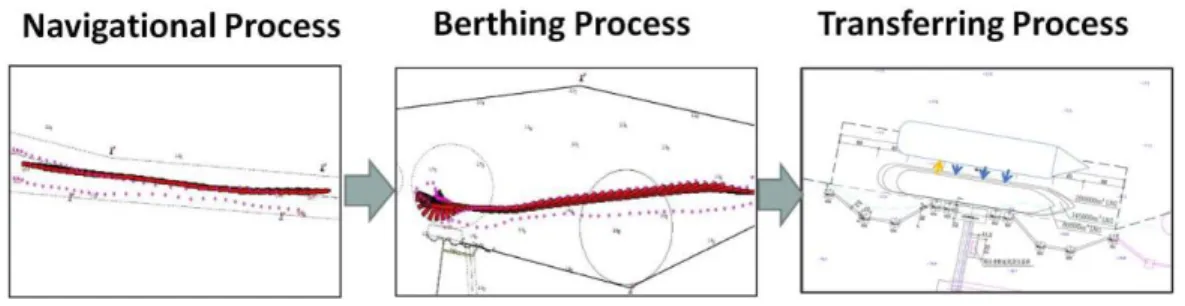
The evaluation process starts with the LNGC entering the inner harbor channel, after the LNGC berthing alongside FSRU and ends with the completion of LNG cargo transferring, see Figure 2.
Figure 2. Defined Evaluation Processes
Three processes are comprised in this research:
• Navigational Safety: LNGC Navigating in the inner harbor channel;
• Berthing Safety: LNGC Berthing operation in the turning basin area;
• Operational Safety: LNG offloading process from LNGC to LNG FSRU.
1.4 Research Methodology
The Multi-attribute decision analysis (MADA) was employed to obtain the preferred decision of building one LNG FSRU system. MADA is an optimum decision-making method to get the output of overall utility function, which is constituted by weight vectors multiplied by utility values. Based on the calculated overall utility value
5
of each alternative, the preferred decision can be made with the maximum expected utility value [6].
Analytic Hierarchy Process (AHP) was firstly proposed by Dr. Saaty in the 1970s to solve decision making problems by evaluating different factors from bottom hierarchy to the highest one [7].
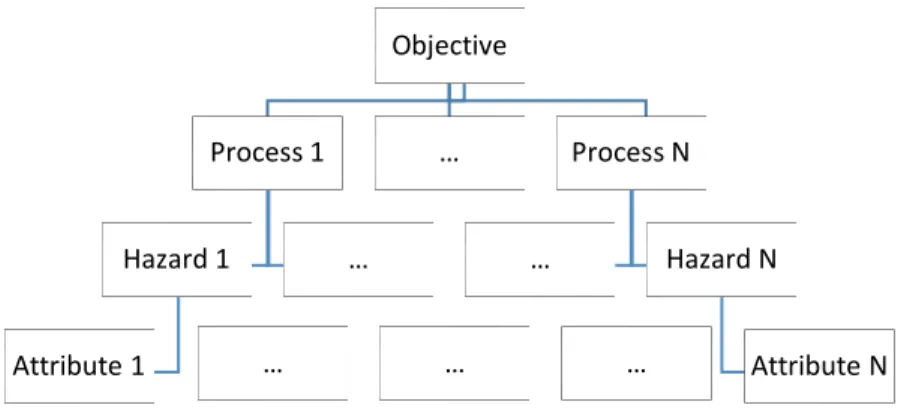
Since the MADA is good at dealing with the decision-making problems among several attributes in one layer, and the AHP outperforms for different layer determination. By putting use of these two theories, this research improved MADA and AHP to a quantitative multi-hierarchy framework MADA (QMFMADA). The core idea of this method to divide the top problem into several processes first, then different processes are evaluated individually by various quantitative tools such as risk simulation software such as Safeti, ship simulator and data analysis software R. Next step is for hazard identification: major hazards are identified under different processes. To quantitatively evaluate different hazards, previous theories and equations may be referred to determine the major attributes which are under the hazard layer. By considering the data availability, the attribute layers can still go down to sub factor layers to quantitatively evaluate the top object directly. Put simply, the framework determination of QMFMADA is a top-to-bottom work, and then the final evaluation is a bottom-to-top progress, see Figure 3.
6
Figure 3. Proposed Evaluation Framework of QMFMADA Objective Process 1 Hazard 1 Attribute 1 … … Process N … Hazard N Attribute N … … …
7
CHAPTER II
LITERATURE REVIEW
2.1 Hazard Identification
To establish the framework shown in Figure 3, it is necessary to determine the hazard hierarchy after the process layer has been defined in Figure 2. Generally, hazards are identified by hazard and operability study (HAZOP), Failure mode, effects and criticality analysis (FMECA), and What-if analysis. According to Paltrinieri, 2015, the typical hazards identified for an LNG-FSRU system are: contact with cryogenic liquid, pool fire, flash fire, rapid phase transition (RPT), stranding, contacting with other objects in the vicinity, and leaking during cargo transferring [8].
8
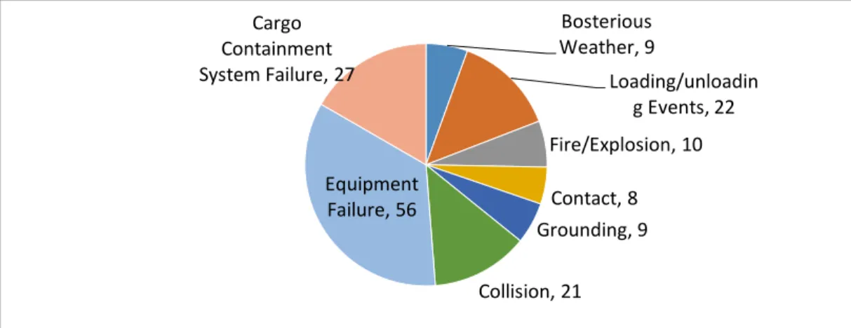
Figure 4. LNGC Accident Category Distribution
*Sources from Houston Law Center, IZAR, Colton Company, DNV report: LNG Accident review and www.seasearcher.com
To establish the LNG-FSRU location evaluation criteria, several factors, such as hydrographic information, navigation safety, fire and explosive risks, exclusion areas, and environment sensitivity, should be taken into consideration individually. Combined with previously recorded incidents, the most threaten hazards, collision, stranding, fire/explosion, and spillage during cargo handling, are selected as evaluation factors of hazard layer in the QMFMADA framework.
From Woodward et al. 2010, the potential fatalities from LNGC operations were estimated as shown in following table.
Bosterious Weather, 9 Loading/unloadin g Events, 22 Fire/Explosion, 10 Contact, 8 Grounding, 9 Collision, 21 Equipment Failure, 56 Cargo Containment System Failure, 27
9
Table 1. Potential Fatalities for Major LNGC Accident Categories by Woodward 2010 [9]
Accident Category Potential Fatalities per Year
Collision 4.42*10-3
Grounding 2.93*10-3
Contact 1.46*10-3
Fire & Explosion 6.72*10-4
Loading/Unloading Events 2.64*10-4
From Table 1, the collision and grounding are the two most severe accidents for LNGC navigation at sea and the contacting usually happened in the harbor areas, leading to third potential fatalities among all accidents. In addition, fire/explosion and loading events should be taken more attention during LNG transferring from LNG carrier to LNG terminal. Therefore, the three processes should be evaluated individually in a quantitative way.
2.2 LNGC Navigational Process
Based on previous research experience, cargo release, collision and grounding are usually considered as major consequences of site specific risk assessment in nautical safety study. As above table mentioned, collision and grounding are selected as the major hazards for LNGC navigation safety phase.
10
2.2.1 Collision Model Fujii’s Model
Researcher Fujii proposed a model to calculate the average number of evasive actions (e.a.) by one ship navigating in one area. Fujii’s Model is [10]:
No. (e. a. ) = ∫entranceexit (ρDeVrel/V)dx (1)
ρ: Traffic density, number of ships per unit area De: Diameter of collision avoidance
V: Speed of passing vessel Vrel: Relative speed
The value of De varies from 9.5 to 16.3 times of ship length, which made the
collision avoidance quite conservative since the minimum shipping distance in some narrow straits are around 3 times of ship’ length overall in the real world.
Macduff’s Model
Another researcher, Macduff, firstly proposed the probable collision model, and the formula is [11]:
P = Pg ∗ Pc (2) Where
-P: the probability that a vessel is involved in a collision accident during its voyage passing one assigned water area
-Pg: the geometrical probability, collision probability without aversive measures are made.
11
-Pc: the causation probability, the conditional probability that a collision occurs in an accidental scenario.
Pg is relevant to geometric parameters of water area, vessel size, traffic volume, course and speed; while Pg is related to mariner’s skills, vessel maneuverability under accident scenarios, and many literatures considered it as a constant. Then for geometrical probability Pg, Macduff’s Model estimated it as follows [11].
Pg = X∙LD2 ∙Sin(θ 2925⁄ ) (3) Where
-D: Average distance between ships -X: Actual length of path for one ship -L: Average vessel length
-V: Ship’s approaching speed, two ships are assumed equal -θ: The angle that one single ship approaching the channel with
The value of Pg will be overestimated when θ is small. The assumption of two ships’ speed being equal made the Pg underestimated.
Pedersen’s Model
To determine the geometrical probability Pg, Pedersen and his research fellows presented a model under a two-channel situation. Channel 1 and channel 2 are assumed as two crossing channels. The equation 4 shows the Pedersen’s collision model [12].
P∆t =Qj(2) Vj(2)fj
2(z
12
-Qj: Number of movements of ship class j per unit time, named as traffic volume
-Z: Distance from the centerline of the fairway
-f: Lateral distribution of the ship routes, often normal distribution -Vij: Relative velocity; -Di, Collision diameter
This model is reasonable for crossing scenario to estimate the geometrical probability due to a more practical assumption. However, the lack of ship movement data made it difficult to determine the probability distribution of ship motion.
In summary, Table 2 shows the expressions and characteristics of each model.
Table 2. Summary of Ship Collision Model
Model Expression Drawbacks
Fujii’s
Model No. = ∫ (ρDeVrel/V) exit
entrance
dx De is conservative (9.5 to 16.3 times ship length), so Pg
is overestimated.
Macduff’s
Model Pg = X ∙ LD2 ∙Sin(θ 2
⁄ ) 925
Pg is overestimated when ɵ is small and
underestimated because of the assumption of two ships are equal speed.
Pedersen’s Model P∆t= Qj(2) Vj(2)fj 2(z j)DijVijdzj∆t
Applicable for crossing channel situation, assume ship lateral motion as normal distribution, not very accurate for head on situation
COWI Model
In order to precisely simulate the head on situation (See Figure 5) in real world, the COWI model is applied to calculate ship collision probability [13].
Px = Pt × Pg × Pc × kRR = LN1N2|V1−V2 V1V2 | × ( B1+B2 c ) × (3 × 10 −4) × k RR (5)
13 L: length of route segment
N1, N2: Number of ship 1, 2 passing per year
V1, V2: Speed of Ship 1 and Ship 2
B1, B2: Breadth of Ship 1 and Ship 2
Pc: Causation probability, taken as a constant 3 × 10⁻⁴
kRR: Risk reduction factor, usually taken 0.5 [13]
Figure 5. Head-on Collision Situation for Two Ships by Li et al., 2012 (Adapted from [13])
As shown in above figure, the overlap area was deemed as the possible collision area with the presupposition of ships’ motion following normal distribution. Compared to other models, the COWI model considered the risk mitigation measure and reduced the uncertainty in some extent by assuming ship motion as normal distribution. Moreover, the most likelihood situation for LNGC navigation in inbound channel is head
14
on situation, so the COWI model was adopted to carry out simulation for LNGC navigation safety phase. It is widely accepted that visibility is a key factor to influence coastal navigation and the leeway and drift angle, which was deemed as a significant parameter to show the vessel’s maneuverability, was largely dependent on the magnitude of wind and current. Therefore, the main parameters to evaluate the collision hazard are determined as wind, visibility and the probability of following current.
2.2.2 Grounding Model
LNGC may suffer from grounding or standing risk when it navigates without sufficient water depth and this risk may bring severe consequence if the sediment of the grounding place is considerably solid. In practice, deck officers should check the water depth reading frequently to make sure the ship has no chance to rush into the shoal when the ship is navigating in harbor areas. The following models are common ones to simulate ship’s grounding.
Fujii’s Model
Similarly, the concepts of geometrical and causation probability were brought to estimate likelihood of grounding as well. Fujii proposed the expected number of groundings (Ng), shown in Equation 6 [10].
NG= PCDρV (6) Where
-Pc: Causation Probability -V: Ship’s speed
15 -ρ: Traffic Density
-D: The width of shoal
Macduff’s Model
Meanwhile, Macduff adopted Buffon’s needle problem to estimate Pg, the equation 7 shows the relationship among Pg, channel width and stopping distance of ships [11].
PG= 4TπC (7)
-C: The width of the channel -T: The ship’s stopping distance
These two above-mentioned models are only affected by the ship particulars and other elements related to location are set to be constant. The uncertainties of the real navigation situation are ignored in most cases, and this model merely considered historical accident data. But this model has been widely used as a basis to improve grounding model.
Pedersen and Simonsen’s Model
Pedersen and Simonsen developed their model to estimate the expected annual number of groundings (Ng), see equation 8 [14].
NG= ∑n class PC,iQie−d/ai
Ship class i ∫ZZminmaxfi(z)dz (8)
Where
-Pc: Causation probability
16
-a: the average time interval of position checks by deck officers -d: the width of channel
-f(): the actual traffic distribution of ships -z: the transverse coordinates of shoals
Table 3 serves a review of above mentioned grounding models, illustrating their expressions and drawbacks.
Table 3. Summary of Ship Grounding Model
Model Expression Drawbacks
Fujii’s Model NG = PCDρV Human factors, ship’s maneuverability and
environmental aspects were all neglected.
Macduff’s
Model PG =
4T πC
Causation probabilities are unknown; this model cannot recommend any risk control option. Traffic density is assumed uniformly.
Pedersen and Simonsen’s model ∑ PC,iQie−d/ai n class Ship class i ∫ fi(z)dz Zmax Zmin
Human factors and ship maneuverability are still neglected and effect of traffic (Q) and ship class (i) are not evidence based.
Montewka’s Model
To overcome those above-mentioned drawbacks, Montewka et al. [15] have proposed a more accurate grounding model with the consideration of the maneuverability of an individual ship and the properties of the traffic. In addition,
17
Automatic Information System was employed to determine the distribution of the ship’s motion.
F = M ×UKCH×r= d×s×cR×b ×UKCH×r (9) -F: threatened Level
-R: radius of Turning Circle
-b: a coefficient that represents the extent of damage to a ship’s hull that occurs when the ship runs aground
-d: a coefficient that represents the distance at which a hazard can be detected -s: a coefficient that represents the accuracy of depth soundings
-c: a coefficient that represents positional accuracy -UKC: under keel clearance
-H: depth of the channel -1/r: distance decay curve
For the LNGC navigation process, the Montewka’s Model was selected as the one to simulate stranding situations since it has a better interpretation and has considered ship maneuverability. Based on the equation 9, the main parameters selected for grounding hazard of navigational process are channel width, channel curvature and under keel clearance.
18 2.3 Berthing Process
When berthing or unberthing operation is taking place, the LNGC shows a characteristic of low speed and large drift angle [16]. Typically, berthing operation for large ships should consider factors such as temperature, berthing ability, wind force, visibility and thunderstorm [17], another researcher Bai presented the berthing influence factors as tug assistance, wind, current, longitudinal speed control, transverse speed control and angular velocity control [18]. What is more, poor communication between crew and marine pilots during berthing operation will probably lead to marine disasters near ports, and the language and cultural diversity of seafarers needs to be considered as well [19].
To evaluate this complicated operation process in a quantitative way, Yang proposed a berthing model by presenting models of ship, propeller and rudder individually and he took full considerations of interactions between each part. As shown in Figure 6, Yang set up two coordinate systems, one is fixed coordinate X0Y0, and the
19
Figure 6. Two Coordinate System of LNGC by Yansheng, 1996 (Adapted from [16])
Where
-m, -mx, -my: ship mass, added mass along x axis, added mass along y axis
-u, -v: line velocity components -r: heading angular velocity -Izz: inertia moment
-Jzz: added inertia moment
-X, -Y: external force along X and Y axis -N: moment of external force
H: ship hull; P: propeller; R: rudder; A: wind; L: mooring line; C: anchor; -S: bank wall; -T: tug.
Based on the above-mentioned theory, LNG ship simulator DMU V-Dragon 3000A was employed to perform a high-precise simulation for LNGC berthing. This simulator adopted a six -freedom motion mathematical model and integrated wind
20
disturbing force model (Equ. 10, 11, 12) and wave force model (Equ. 13, 14, 15) as the key ones for external force [20].
Wave Disturbance Model
XA =12ρAAfUR2C Xa(αR) (10) YA =12ρAAsUR2C Ya(αR) (11) NA =12ρAAsLoaUR2C Na(αR) (12)
-Cxa(αR), -Cya(αR), -Cna(αR): wind pressure coefficients -As: Lateral projection area at waterline
-Af: Conformal projection area at waterline Secondary Order Wave Force Model
XW2 = 12ρLa2cos(χ) C XW(λ) (13) YW2 = 12ρLa2sin(χ) C YW(λ) (14) NW2 =12ρL2a2sin(χ) C NW(λ) (15) Where
-Cxw(λ), -Cyw(λ), -Cnw(λ): experiment coefficients -a: wave amplitude
-χ: wave direction angle -λ: wave length
To evaluate the LNGC berthing operation, six main parameters were determined by the equations 10-15, they are : water depth of turning basin, following current speed,
21
berth length, radius of turning area, transverse wave height and the probability of crossing wind (beam wind).
2.4 LNG Transferring Process
After the berthing process is completed, the LNG should be transferred from LNGC to LNG FSRU, which is a typical Ship to Ship LNG transferring process. Two common solutions for Ship to Ship transferring process, one is called side-by-side transferring pattern, and the other is called tandem transferring pattern [21]. There are three liquid transferring connection hoses and one vapor counterflow connection hose in the Figure 7.
Figure 7. Ship to Ship Pattern for LNG FSRU System
Besides the preparation work prior to transferring operation, the typical STS process should include: mooring to the FSRU, water curtain switch on, connecting
22
transferring hose, inerting of LNG fuel hose and transferring arm, cool down transferring hose, oxygen test, leak test, Emergency Shut Down System (ESDS) test under normal and low temperature, leakage and temperature monitoring during transferring, and post processing actions such as draining, methane purging for liquid line and vapor line, measurement after transfer and transferring hose disconnection [22].
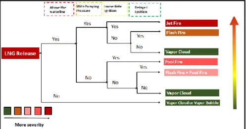
For the LNG FSRU system, many causes would result in LNG accidental release such as FSRU or LNGC tank breach, connection pipe rupture and LNG vaporizer failure. Furthermore, possible associated consequences of LNGC release on water have been identified as BLEVE, vapor cloud explosion (VCE), jet fire, flash fire, pool fire, RPT, cryogenic burns, etc. Figure 8 shows a simplified bow-tie diagram for LNG accidental release to consider both the causes and the outputs of the top event [5, 9, 23].
23
As shown in above bow-tie diagram, five causes may result in LNG accidental release for the LNG FSRU system: FSRU storage tank breach, connection hose rupture, connection flange failure, LNG Tank breach and LNG vaporizer failure. To simulate the most probable leading factors of LNG transferring process, two events, connection hose rupture and connection flange failure, were identified as a result of their high-risk characteristic. During LNG transferring process, the accidental release of LNG could lead to many possible consequences. When LNG is released under the waterline, it may probably convert to vapor bubble, then LNG bubble may escape above the waterline to produce LNG vapor. For above-waterline release, jet fire, flash fire and pool fire may form under different scenarios. The following figure is the event tree analysis for LNG accidental release [9, 24, 25, 31].
24
As above mentioned, events of connection hose rupture and connection flange failure were identified to list on the hazard layer of the final framework. In addition, as shown in Figure 9, the possible fatality related consequences are flash fire, pool fire and jet fire, since the explosion is not likely to occur in the open water area [26, 31].
After the two events and relevant consequences were identified, the dispersion models and the fire models were needed to process flammable calculations. The flammable calculations include fireballs (instantaneous releases), jet fires (pressurized releases), pool fires (after rainout), and vapor cloud fires or explosion. This study adopted the Unified Dispersion Model (UDM) as the core model to research the dispersion effects of LNG releasing on water, which is also widely applied in the hazard assessment software package Phast and Safeti [42].
2.4.1 Dispersion model
In this research, crosswind situation was selected as a risk-seeking scenario to evaluate the LNG FSRU system. To simulate crosswind situation, three consecutive phases were adopted for two scenarios which were instantaneous release and continuous release.
Phase 1, Jet Spreading
The cloud is assumed to remain circular until the passive transition or until the spread rate reduces to the heavy-gas spread rate, [42]
𝑅𝑦 = 𝑅𝑧 (16) Where
25 Phase 2, Heavy-gas Spreading
After the jet spreading phase, the heavy-gas spreading phase served as the second one.
For instantaneous dispersion,
𝑑 𝑅𝑦 𝑑𝑡 = 𝐶𝐸 𝐶𝑚√ 𝑔{max[0,𝜌𝑐𝑙𝑑− 𝜌𝑎(𝑧=𝑧𝑐𝑙𝑑)]}𝐻𝑒𝑓𝑓(1+ℎ𝑑) 𝜌𝑐𝑙𝑑 , 𝐶𝑚 = [Γ (1 + 2 𝑚)] 1⁄2 (17) For continuous dispersion,
𝑑 𝑅𝑦 𝑑𝑥 = 𝐶𝐸 𝑢𝑥𝐶𝑚√ 𝑔{max[0,𝜌𝑐𝑙𝑑− 𝜌𝑎(𝑧=𝑧𝑐𝑙𝑑)]}𝐻𝑒𝑓𝑓(1+ℎ𝑑) 𝜌𝑐𝑙𝑑 , 𝐶𝑚 = Γ (1 + 1 𝑚) (18) Where
-Cm = 1.15, Van Ulden cross-wind spreading parameter
-Heff: effective height of cloud after full touchdown
-hd: fraction of bottom half of cloud which is above ground
-Cm: conversion factor between cloud half-widths
-CE: parameter in gravity-spreading law
-m: exponent of horizontal distribution function for concentration -ρa: density of ambient air
- ρcld: density of plume
-ux: horizontal component of cloud speed
-z: vertical height above ground
-zcld: height above ground of cloud centerline
26
After the jet spreading and heavy-gas spreading, the passive spreading was applied, and the equations are as follows [42].
𝑑 𝑅𝑦 𝑑𝑡 [𝑎𝑡 𝑥] = 𝑢𝑥√2 𝑑 𝜎𝑦𝑎 𝑑𝑥 [𝑎𝑡 𝑥 − 𝑥0] instantaneous (19) 𝑑 𝑅𝑦 𝑑𝑥 [𝑎𝑡 𝑥] = √2 𝑑 𝜎𝑦𝑎 𝑑𝑥 [𝑎𝑡 𝑥 − 𝑥0] continuous (20) Where
-x: horizontal downwind distance
-σya: standard empirical correlation for passive crosswind dispersion coefficient
2.4.2 Fire Model
Typically, there are three types of fires related to LNG spillage on the water, jet fire, pool fire and flash fire.
The jet fire in this research was produced by a liquefied/ two phase natural gas. The effective source diameter of the flame is significant to correctly simulate the effect zone of jet fire. The following equation is the expression of effective source diameter (Ds) [55].
𝐷𝑠 = 2𝑟𝑗√𝜌 𝜌𝑗
𝑣𝑎𝑝[𝑇𝑠𝑎𝑡(𝑃𝑜)] (21)
Where
-rj: expanded radius of the escaping fluid -Po: atmospheric pressure
- ρvap[Tsat(Po)]: the saturated vapor density of the fuel at ambient pressure - ρj: Density of expanded fluid jet
27
Besides jet fire, pool fire is another possible fire type when releasing on the water. To determine the magnitude of the surface emissive power of pool fire, the following equation is adopted [56].
𝐸𝑓 = 𝐸𝑚 [1 − 𝑒−𝐿𝑠𝐷] (𝐿𝑢𝑚𝑖𝑛𝑖𝑢𝑠 𝐹𝑖𝑟𝑒𝑠) = 𝐸𝑚 [𝑒− 𝐷 𝐿𝑠] + 𝐸𝑠 [1 − 𝑒−𝐿𝑠𝐷] (Sooty Fires) = 𝜒𝑅𝑚Δ𝐻𝑐 [1+4𝐻𝐷] (𝐺𝑒𝑛𝑒𝑟𝑎𝑙 𝐹𝑖𝑟𝑒𝑠) (22) Where,
-Em: Maximum emissive power for luminous fires -Es: Smoke emissive power
-Ls: A characteristic length for decay of surface emissive power -χR: The ratio of the total energy radiated to the total energy released -D: Diameter of the flame
-H: Height of the flame
The equation for “general fires” was applied when the experimental data were not available.
28
CHAPTER III
METHODOLOGY AND FRAMEWORK DEVELOPMENT
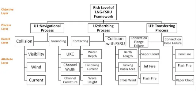
To establish the evaluation framework as shown in Figure 1, the layers should be determined from top to bottom. The second layer is filled with three processes defined in chapter I: LNGC Navigation Process, Berthing Process and LNG Transferring Process. Then the third layer, identified hazard layer, was determined by chapter II.
3.1 Framework Development
For the navigational process, collision and grounding are the major hazards for LNGC, and from Equation 5, visibility, wind and current are the attributes to lead to collision. Similarly, the major parameters in Equation 9, i.e., UKC, Channel Width and Channel Curvature, are the attributes to result in LNGC aground.
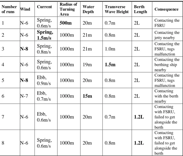
For berthing process, DMU ship simulator was adopted to analyze the attributes. The extreme conditions were selected as the input parameters: the wind direction was blowing to the shore, North; the radius of turning area was set as 500 meter and 1000 meter, respectively; the berthing length was set 1.2 times and 2 times ship’s length overall; and other values of parameters were obtained when the incident happened. Two scenarios were designed to determine the most influential factors:
29
1. Full loaded, port side berthing with spring tidal current; 2. Full loaded, starboard side berthing with ebbing tidal current.
The failure simulation runs were shown in Table 4.The major consequences of berthing process were contacting with obstruction and collision with the FSRU, the offshore “pier”.
Table 4. Simulation Results of Ship Simulator for Berthing Process Number of runs Wind Current Radius of Turning Area Water Depth Transverse Wave Height Berth Length Consequence 1 N-6 Spring, 0.6m/s 500m 20m 0.7m 2L Contacting the FSRU 2 N-6 Spring, 1.5m/s 1000m 21m 0.8m 2L Contacting the jetty nearby 3 N-8 Spring, 0.8m/s 1000m 21m 1.0m 2L Contacting the FSRU, tugs malfunction 4 N-6 Spring, 0.6m/s 1000m 19m 1.5m 2L Contacting the berthing ship nearby 5 N-8 Ebb, 0.9m/s 1000m 20m 0.8m 2L Contacting the FSRU, tugs malfunction 6 N-7 Ebb, 0.7m/s 1000m 15m 0.8m 2L Contacting with the berth nearby 7 N-6 Ebb, 0.6m/s 1000m 20m 0.7m 1.2L Contacting with FSRU, failed to get alongside the berth 8 N-6 Spring, 0.6m/s 1000m 20m 0.8m 1.2L Contacting with FSRU, failed to get alongside the berth
30
Based on the simulation results by DMU V-Dragon 3000A ship simulator, the most significant parameters leading to LNGC contacting with the nearest obstruction are water depth in that area, transverse wave height of turning area and the magnitude of following current; while the attributes for contacting between LNGC and LNG FSRU are berth length, radius of turning basin area and the probability of crossing wind.
For LNG transferring process, vapor cloud, pool fire, flash fire and jet fire may be the outputs of the connection flange failure and connection hose failure. Therefore, the final framework of QMFMADA is established accordingly, see Figure 10.
31 3.2 Parameters Determination
After the final framework was determined by adopting a top-to-bottom strategy, the evaluation work can be processed from an adverse way, attribute layer goes first. In this study, the whole LNG FSRU system comprised one LNG carrier, one LNG floating receiving terminal and the interact operation between them. So, the characteristics of LNGC and LNG FSRU should be determined as a preparation work. Recent years, two most common large-scale LNG ship type, Q-Flex and Q-Max, were widely used all over world for LNG long distance transiting. To consider the current trend for LNG offshore application, Q-Flex was applied in this study as the input ship type of ship simulator DMU V-Dragon 3000A, and the dimension of its receiving terminal FSRU was employed accordingly [27], see Table 5.
Table 5. Parameters of LNGC and FSRU
Parameters LNGC(Q-Flex) FSRU
LOA 303 315
Loading Capacity 142933.7 m3 217000 m3
Breadth 50 50
Draft 12 12.5
Referred from the previous reports, the loading / unloading equipment of FSRU have 4 liquid loading hoses and 2 vapor return hoses, each of them has one spare part.
32
The maximum loading capacity, length of LNG loading hoses and other parameters are listed in Table 6 [28].
Table 6. Parameters of FSRU’s Loading Equipment [28]
Parameter Value
Maximum Loading Capacity 8000 m3/h for all loading hoses
Maximum Unloading Capacity 5000 m3/h for all loading hoses
Number of LNG Loading Hoses 4 (1 spare)
Number of Vapor Return Hoses 2 (1 spare)
Inner Diameter of LNG Loading Hoses 0.254 m
Length for LNG Loading Hoses 18.5 m
Inner Diameter of LNG Loading Hose Flange 0.41 m
Inner Diameter of Vapor Return Hose Flange 0.41 m
As shown in Table 6, the value of maximum loading capacity will be applied to determine the estimated release volume and the diameter of LNG loading hoses and loading hose flange were utilized as the key factors to define scenarios for consequence analysis in the following chapters.
33
CHAPTER IV
CASE STUDY FOR DEFINED SYSTEM
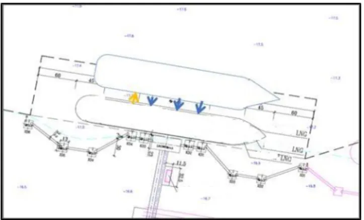
To find out a favorable position to build LNG FSRU system, two locations from China were applied to carry out case study based on the proposed framework. One location is New Port of Dalian, northern part of China; the second one is Qidong Port of Nantong, the East China Sea, shown in Figure 11.
Figure 11. Two Alternative Locations for LNG FSRU System
The proposed LNG FSRU layout maps of two locations were drawn in Figure 12. The proposed LNG FSRU for Dalian locates at the south edge of the coast line while the
34
proposed one for Nantong locates at the northeast side of the coast line. The harbor layout maps of two locations were shown in Figure 12 by Google Map.
Figure 12. Harbor Layout Maps for Two Alternative Locations
The yellow arrows in Figure 12 showed the exact positions for the LNG FSRU. The proposed direction of location A is 053°~233°, berth length is 446 meters (m); the design direction of location B is 099°~279° and berth length is 430 m. Figure 13 showed the parametric design for two locations by Auto CAD.
35
After the dimension of two proposed locations were determined, the evaluation steps can be processed from LNGC navigating in the inbound channel to the LNG successfully transferring from LNGC to LNG FSRU.
4.1 Data Collection for Navigational Process
The left side figure is the layout map of location A (Dalian proposed LNG FSRU), while the right one is the layout map of location B (Nantong proposed LNG FSRU). To evaluate the framework of QMFMADA, the bottom-to-top sequence should be adopted, so the factors of very bottom attribute layer for navigation process are visibility, wind and current.
Considering the data availability for attributes of collision hazard, the visibility parameter is determined by number of days under poor visibility (visible distance < 4000m) per year; the wind parameter is determined by Number of days under standard wind scale, which is equal to number of days under Beaufort scale 6 and 7 plus 1.5 times number of days under Beaufort scale 8 or more [29]; and the parameter current is determined by the probability of following current, which is the most difficult situation for ship maneuvering. For grounding hazard, the attribute channel width and channel curvature can be determined directly by the actual channel data, and the minimum under keel clearance (UKC) is equal to the minimum chart water depth minus actual draft of LNGC. The actual values of navigation process related attributes for two alternatives are shown in Table 7.
36
Table 7. Values of Navigational Process Related Attributes for Two Locations Channel Width Channel Curvature UKC Windy Days Following Current Prob. Visibility Location A 1050m 31° 12m 140 7.6% 22 Location B 690 m 27° 5m 151 9.3% 30
Referred from the Code for Design of Liquefied Natural Gas Port and Jetty [30], the limited conditions for ship’s navigating in channel were regulated as follows.
Wind speed should not exceed 20m/s and the transverse waves should be less than 2.0 meters, while the magnitude of following waves should not exceed 3.0 m; Visibility for LNGC navigating in the inbound channel should be greater than 2000 meters and the upper limit for transverse speed of current is 1.5 m/s, while the following current speed should not exceed 2.5 m/s.
4.2 Data Collection for Berthing Process
For the second process, berthing process simulation, the water depth for the contacting possibility for LNGC and other navigation obstruction is the minimum water depth in berthing area; “Following Current” is the magnitude of following current during berthing operation; while the transverse wave height can be directly obtained from the hydrographic data of two harbor authorities. For the hazard of possible collision with FSRU, the berth length and turning basin area is the values of designed berth length and radius of turning water shown in Figure 12, and the crossing wind, which is defined as
37
the wind blowing the LNGC toward FSRU side, was evaluated by the wind rose maps of two locations. Therefore, the values of berthing process related attributes are shown in Table 8.
Table 8. Values of Berthing Process Related Attributes for Two Locations Water Depth Following Current Wave Height Berth Length Radius of Turning Area Crossing Wind Prob. Location A 20 m 0.8m/s 1.08 m 1.5L 1020m 4.6% Location B 17m 0.85m/s 0.81 m 1.25L 1260m 3.8%
In addition, the Code for Design of Liquefied Natural Gas Port and Jetty [30] was referred to adjust the environmental input data for berthing process simulation. The code regulated berthing limited conditions as follows: The maximum allowable wind speed should be 15 m/s; The transverse waves should not exceed 1.2 meters, while the threshold value of following waves should be 1.5 m; Visibility for navigating in the inbound channel should be greater than 1000 meters; The upper limit for transverse current speed is 0.5 m/s, while the following current speed should not exceed 1.0 m/s.
4.3 LNG Transferring Process Simulation
After the LNGC is safely getting alongside the LNG FSRU, the system moves to the last stage, LNG transferring from LNGC to FSRU.
38
4.3.1 Defined Scenarios
Based on the previous research [32, 33, 34], it is a reasonable to simulate this event “LNG releasing on the water” by two scenarios: one is called maximum credible scenario (MCS), which is the most possible scenario for one year the LNG FSRU system may face; another one is called worst case scenario (WCS), which means the extremely dangerous situation for LNG FSRU system [35].
To process the simulation by Safeti 7.2, several input parameters should be determined. For the two scenarios, the external environment factors for weather data input, wind, air temperature and relative humidity, can be obtained from the meteorological and hydrographic records of two locations.
For maximum credible scenario, the input parameter “wind” was the prevailing wind for two locations. As shown in Figure 14, the wind rose map of location A shows the prevailing wind direction was north wind with the speed of 8 m/s; while the prevailing wind direction of location B is northeast wind with the speed of 6.7 m/s; the air temperature for MCS was the average temperature of one whole year, where 10.5 degree centigrade for location A and 15.1℃ for location B; similarly, the humidity parameter was selected as the average humidity for a whole year, 69% for location A and 75% for location B.
39
Figure 14. Wind Rose Map of Location A (Adapted from [57])
Table 9. Wind Direction Frequency Distribution (Adapted from [57])
Average Speed (m/s) Max. Speed (m/s) Frequency (%)
N 8.0 34.2 19.5 NNE 5.6 20.0 2.8 NE 3.7 17.0 1.2 ENE 5.7 17.0 2.9 E 4.8 15.0 4.9 ESE 4.2 11.5 6.8 SE 3.8 22.0 6.4 SSE 4.2 12.0 6.8 S 4.9 12.0 9.0 SSW 5.7 13.0 3.8 SW 5.5 14.0 4.5 WSW 5.5 13.0 2.6 W 5.5 17.0 4.0 WNW 6.6 20.0 3.4 NW 6.5 24.4 8.8 NNW 7.5 33.8 5.8 CALM 6.8
For worst case scenario, the “wind” parameter was the most hazardous when the wind is blowing toward the pier since the fire may get more assets and people involved.
40
By considering the wind rose map of each location, the most hazardous wind directions were southeast and northeast for location A and location B, respectively and the worst wind speed is 15m/s because it is the maximum speed to still allow LNG transferring operation to process [30]. Since the air temperature may fluctuate day to day, the WCS air temperature was chosen as the highest monthly average one for a whole year, 15.1℃ for location A and 20.6℃ for location B. Similarly, the humidity parameter was determined as the highest monthly average humidity for a whole year, 83% for location A and 88% for location B.
The release preconditions, hose loading capacity, leakage time and hole size, were determined as the main parameters to define the exact releasing volume of MCS and WCS. For WCS, the hose loading capacity was referred as the LNG FSRU’s maximum loading capacity and the accidental release time was determined as 20 minutes to calculate the simulated release volume for the events as connection hose rupture and flange failure. As shown in table 5, the inner diameter of LNG loading hose and loading hose flange were 0.254 m and 0.41 m, respectively, so the hole size was determined as the total-damage scenario. For MCS, the hose capacity was determined as the 87% of the maximum loading capacity and the release time was the 10 minutes; the holes was determined as 0.2 m for connection flange failure and 0.12 m for connection hose rupture scenario. The input data for MCS and WCS simulation are listed in Table 10.
41
Table 10. Input Data for Safeti Simulation Plans
Wind Air Temperature Humidity Pasquill Stability Release Time Hole Size Diameter Maximum Credible Scenario (MCS) Prevailing Wind (A; 8 m/s, N; B:6.7m/s, NE) Yearly Average (A: 10.5℃; B:15.1℃) Yearly Average Humidity (A: 69%; B: 75%) E 1167 m3 0.2m (Flange Failure)/0.12m (Hose Rupture) Worst Case Scenario (WCS) 15m/s (A: SE; B: NE) Highest Monthly Average Temperature (A: 15.1℃; B: 20.6℃) Highest Monthly Average Humidity (A: 83%; B: 88%) Loc. A: C; Loc. B: D 2667m3 0.41 m (Flange Failure)/0.254 m (Hose Rupture) 4.3.2 Simulation Results
The runs were designed in 4 group comparisons with 8 simulations. Simulation plan 1, 2, 3 and 4 were taken for connection flange failure. Among these four simulation plans, simulation plan 1 and 2 took place in location A under scenario MCS and WCS, respectively; Simulation plan 3 and 4 took place in location B under scenario MCS and WCS. Meanwhile, simulation runs 5 to 8 were for connection hose rupture, and simulation plan 5 and 6 took place in location A under scenario MCS and WCS; Simulation plan 7 and 8 took place in location B under scenario MCS and WCS, respectively.
Figure 15 shows the preliminary simulation outputs by Safeti 7.2 for two alternatives under the condition of “flange failure with worst case scenario” (simulation plan 2 and 4).
42
Figure 15. Simulation Outputs for Two Alternatives under WCS and Flange Failure
From Figure 15, the left one is the simulated thermal radiation influence areas of location A and the right one is that of location B. The red circle is the high thermal radiation area with heat flux 37.5 kW/m2, the green one is the thermal radiation intensity
of 12.5 kW/m2 and the blue circle is the range of thermal radiation intensity of 5kW/ m2.
Meanwhile, other simulation plans were taken under different input data, and Table 11 shows all simulated outcomes of eight simulation plans. The potential fatalities would be calculated based on the values of thermal radiation distance and flammability limits distance in the following chapter.
43
Table 11. Outcomes of Designed Simulation Plans
Plan Location Scenario Dia. of Hole Size (mm) Est. Leakage Volume Fire Type
Thermal Radiation Distance Flammability Limits Distance 4kW/m2 12.5kW/m2 37.5kW/m2 UFL LFL 0.5LFL 1 A MCS 200 1167 Flash 220 794 1590 2 A WCS 410 2667 Jet 1141 1022 976 3 B MCS 200 1167 Flash 194 771 1546 4 B WCS 410 2667 Jet 1128 1016 976 5 A MCS 120 1167 Flash 11 77 277 6 A WCS 254 2667 Pool 501 302 192 7 B MCS 120 1167 Flash 9 70 202 8 B WCS 254 2667 Pool 722 525 222
44
CHAPTER V
EVALUATION RESULTS AND DISCUSSION
After the completion of simulation runs for three processes, the utility value should be determined from bottom hierarchy to the top. Navigational process and berthing process, which were called maritime safety study in this research, adopted risk evaluation matrix to determine each utility value; while for chemical process safety part, LNG transferring process was determined by the potential loss of life (PLL) [36].
5.1 Evaluation Methodology for Maritime Safety Study
In order to establish the relationship between expected utility value and risk level, five qualitative evaluation scales (favorable, acceptable, moderate, limited acceptable, and unacceptable) are converted to five utility ranges evenly. 90 experts were consulted to determine the evaluation standards for each attribute of navigational process and berthing process shown in Figure 10.
To avoid subjectivity, 30 senior officers of deck department aboard ships, 30 professional pilots and 30 professors from marine maneuvering major built up the expert judgment team for this research. Based on the opinions of the expert judgment team and previous studies on the marine maneuvering, every individual attribute was evaluated quantitatively based on the risk utility value (RUV) or risk tolerance index, which was
45
distributed evenly from 0 to 1 with the interval of 0.2. Furthermore, risk utility value range from 0.8 to 1.0 means the environment of this location is favorable to build LNG FSRU, while the value locating between 0.6 and 0.8 means it is acceptable for LNG FSRU; the range 0.4 to 0.6 means moderate environmental conditions for the system; limited acceptable when the RUV is in the range of 0.2 to 0.4; it is unacceptable when the utility value goes below 0.2 [40].The evaluation standards for adopted attributes of navigational and berthing process were established based on the questionnaires (see Appendix 1) collected from professors, pilots and senior officers onboard.
5.1.1 Evaluation Standards for Risk Utility Value
“Visibility”, as an example, was determined by the number of days under poor visibility (visible distance < 4000m) per year [29, 37]. Four risk utility values (0.8, 0.6, 0.4 and 0.2) were given to experts to get their opinions on the risk standard of “visibility” to build LNG FSRU. From the collected data, Figure 10 showed the distributions of restricted visibility days per year where it is favorable/ acceptable/ moderate / limited acceptable/ unacceptable for LNG FSRU operations.
46
Figure 16. Data Analysis of Boundary Values of “Visibility”
Since there were some outliers among these four graphs, the new distribution without outliers can be shown on the Figure 15. Therefore, the point value of these four risk utility values with 95% confidential interval can be (14.47, 15.64), (19.68, 20.70), (29.15, 30.22) and (39.77, 40.65) with the p value much smaller than 0.05, shown in Appendix 2. Therefore, the evaluation standard for “visibility” was shown on Table 12.
Risk Utility Value = 0.8 Risk Utility Value = 0.6
Risk Utility Value = 0.4
47
Table 12. Evaluation Standard for “Visibility” Utility Range Factors Favorable, (0.8,1] Acceptable, (0.6,0.8) Moderate, (0.4,0.6] Limited Acceptable, (0.2,0.4] Unacceptable, [0,0.2] Visibility <15 15~20 20~30 30~40 >40
The total evaluation standards based were displayed in the Table 13 by analyzing the collected data for all the attributes of navigational process and berthing process.
Table 13. Evaluation Standards for Each Attribute of Maritime Safety Study Utility Range Factors Favorable, (0.8,1] Acceptable, (0.6,0.8) Moderate, (0.4,0.6] Limited Acceptable, (0.2,0.4] Unacceptable, [0,0.2] Visibility (d/y) <15 15~20 20~30 30~40 >40 Windy Days (d/y) <30 30~60 60~100 100~150 >150 Following Current Prob. < 3% 3~6% 6~10% 10~15% >15% Channel Width >900 650~900 450~650 300~450 < 300 Channel Curvature <15° 15°~25° 25°~35° 35°~45° >45° UKC >15m 10~15m 5~10m 2~5m <2m Water Depth >25m 22~25m 18~22m 15~18m <15m Following Current <0.3m/s 0.3~0.6 0.6~0.8 0.8~1 >1m/s Wave Height <0.3m 0.3~0.6 0.6~1.0 1.0~1.2 >1.2m Berth Length >2.5L 2~2.5L 1.5~2L 1.2~1.5L <1.2L Turning Basin Area >1200m 1000~1200 m 800~1000 m 600~800 m <600m Cross Wind Prob. < 1.5% 1.5~3% 3~4.5% 4.5~6.5% >6.5%
48
5.1.2 Risk Utility Value Analysis
To get the expected value of each attribute for both alternatives, the utility value for the bottom hierarchy should be calculated first. Ua(Collision) was taken as an example, the value of it should be calculated by attributes “visibility”, “windy days” and “following current probability”. Based on expert judgment records, the utility function for “visibility” can be obtained by the statistics software R.
Firstly, the total data were split into three parts, 45 data points for training data, 10 data points for validation data set and 35 data points for testing data. From the output of plot command, one outlier (Vis=45, Risk=0.6) and one leverage (Vis=125, Risk=0.05) were identified, then the new data set were established without those two data points.
Suppose the data points following linear regression, the regression function should be:
Risk = β0+β1Vis+…+βnVisn (23)
Five regression functions were tried for “Visibility” by R, shown in Appendix 3 (Figure 1~5). Table 14 showed all the summaries about these five regression models for “Risk ~ Visibility”.
49
Table 14. Summary of Five Possible Regression Functions R Square Value Coefficients Comments Risk= β0+β1Vis 0.77 β0 = 0.83 β1 = -0.011
The least R square value; The standard residual plot showed the linearity and heteroscedasticity were not good; The scale-location plot showed a curve with non-equally spreading residuals
Risk= β0+β1In(Vis)
0.93 β0 = 1.931
β1 = -0.438
The standard residual plot showed the linearity and heteroscedasticity were not good; The scale-location plot showed the residual spreading equally along the ranges of predictors; But the Cook’s distance line was a broken line.
Risk= β0+β1Vis+ β2Vis2 0.96 β0 = 1.251 β1 = -0.035 β2 = 2.56*10-4
The standard residual plot showed the linearity and heteroscedasticity were good; The scale-location plot showed the residual spreading equally along the ranges of predictors; But the Cook’s distance line was close to a line with one point locating between 0.5 and 1. Risk= β0+β1Vis+ β2Vis2 +β3Vis3 0.98 β0 = 1.464 β1 = -0.055 β2 = 7.49*10-4 β3 = -3.44*10 -6 See Figure 17. Risk= β0+β1Vis+ β2Vis2+β3Vis3 +β4Vis4 0.98 β0 = 1.362 β1 = -0.041 β2 =1.87*10-4 β3 =5.34*10-6 β4 =-4.59*10-8
The largest R square value; P value ofβ2, β3 and β2
were much largerthan 0.05; The standard residual plot showed the linearity and heteroscedasticity were good; The scale-location plot showed the residual spreading equally along the ranges of predictors; But the Cook’s distance line was close to a line with one point locating close to 1.
According to the column of “R-square value”, the last two functions were the best among all five models as per their good interpretation for existed data points. However, interpretation and prediction should be balanced to get an optimal model by the comprehensive performances, and Figure 17 showed the performance of the fourth function.
50
Figure 17. Data Testing Performance of Selected Model
The standard residual plot of Figure 17 showed the linearity and heteroscedasticity were good; the normal quantile plot showed the data were normally distributed; the scale-location plot showed the residual spreading equally along the ranges of predictors; and the Cook’s distance line was close to a straight line without any leverage.
Therefore, our model for “Visibility” is:
Risk = Vis+I(Vis^2)+I(Vis^3)= 1.464-0.055Vis+ 7.49*10-4 Vis2 -3.44*10-6 Vis3 (24)
Then the model was validated by applying K-fold cross validation (k=5), shown in Appendix 3 (Figure 6). Finally, the rest of the dataset were used to test the model. The mean value and standard deviation of the prediction were calculated to prove that the accuracy of our model was acceptable.
51
Therefore, by inputting the “Visibility” data into the model, the risk utility value for location A: Ua(V) = 0.5803 while the RUV for location B: Ub(V) = 0.3952. By the same process, the RUV of “windy days”, Ua(W) = 0.2321 and Ub(W) = 0.1991; the RUV of “Following Current Probability”, Ua(C) = 0.5218 and Ub(C) = 0.4281.
5.1.3 Weight Value Determination
The same methodology was applied to get the utility values of “windy days” and “following current Probability”. Then the AHP was adopted to calculate weight values of each attribute. By applying pairwise comparison, the weight evaluation matrix of “Collision” can be obtained as shown in Table 15.
Table 15. Weight Evaluation Matrix of “Collision”
Evaluation Index K1 K2 K3 K1, Visibility 1 1.37 4.35 K2, Windy Days 0.73 1 2.86 K3, Following Current Prob. 0.23 0.35 1
By calculation, the maximum eigenvalue of evaluation matrix is λmax = 3.0018,
and the weight vector (eigenvector) can be obtained accordingly. After normalizing, the weight vector is WA =(0.5146,0.3628,0.1226). Therefore, the consistency index is given as:
![Figure 1. LNG Supply Chain (Adapted from [4])](https://thumb-us.123doks.com/thumbv2/123dok_us/1420551.2690130/13.918.161.780.580.697/figure-lng-supply-chain-adapted.webp)
![Figure 5. Head-on Collision Situation for Two Ships by Li et al., 2012 (Adapted from [13])](https://thumb-us.123doks.com/thumbv2/123dok_us/1420551.2690130/24.918.280.663.481.717/figure-head-collision-situation-ships-li-et-adapted.webp)