Kernel methods for advanced
Statistical Process Control
Issam Ben Khedhiri
Doctoral Thesis
in partial fulfilment of the
requirements for the Degree of
“Doktor der Naturwissenschaften”
in the Department of Statistics
University of Dortmund
Prüfungskommission:
Prof. Dr. Jörg Rahnenführer (Vorsitzender) Universität Dortmund
Prof. Dr. Claus Weihs (Gutachter) Universität Dortmund
Prof. Dr. Joachim Kunert (Gutachter) Universität Dortmund
Prof. Dr. Mohamed Limam (Gutachter) University of Tunis
Dr. Dr. Marco Grzegorczyk (Beisitzer) Universität Dortmund
Acknowledgment
I would like to express my sincere gratitude to my supervisors Professor Claus Weihs and Professor Mohamed Limam. This thesis would not have been possible without their encouragement, guidance and support. I am deeply indebted to the Deutscher Akademischer Austausch Dienst (DAAD) for financing my study and for giving me the chance to conduct my research in such high quality environment. Many thanks go to my DAAD coordinator Mrs Cornelia Hanzlik-Rudolph for her valuable help and advice. I would also like to acknowledge my colleagues Bj¨orn Bornkamp and Adrian Wilk for helping me with valuable advice during the start of my study at the University of Dortmund. I am heartily thankful to Mrs Sabine Bell for her great efforts throughout my stay at the university. Lastly, I would like to thank my family for their support. I am greatly and forever indebted to my parents for their love and generosity throughout my entire life.
List of Figures
1.1 Illustration of Hotelling’s T2 control chart . . . . 15
2.1 Basic idea of Kernel PCA . . . 23 3.1 Comparison of computation cost for different numbers of
prin-cipal components p with n equal to 1000 and N equal to 10 . . 40 3.2 Computation cost in relation to the size of data block N with
n equal to 1000 and p equal to 10 . . . 40 3.3 Time needed to update the KPCA model using batch SVD
and block updating . . . 42 3.4 Time needed to update the KPCA model using single updating
and block updating . . . 42 3.5 Comparison of reconstruction errors of different updating
meth-ods . . . 43 3.6 Relative errors of the first 10 principal components calculated
by the difference between eigenvalues obtained by batch SVD and block updating . . . 44 4.1 Illustration of the simulated multivariate nonlinear process . . 49 4.2 Batch PCA and KPCA monitoring charts in the case of
nor-mal operating condition. The blue and red lines represent respectively the value of the control statistic and its limit . . . 51 4.3 Adaptive PCA and KPCA based monitoring charts in the case
of normal operating condition . . . 52 4.4 Adaptive PCA and KPCA based monitoring charts in the case
of Fault 4, where the fault starts after observation 100 . . . . 4.5 Illustration of the non-stationary behaviour for some variables
of Tennessee Eastman process . . . 55 4.6 Cross-validation errors and Percent of explained variance for
different numbers of Principal Components . . . 56 4.7 Monitoring chart in case of Fault 9 (Q statistic) and Fault 4
(T2 statistic) . . . . 58
5.1 Error lying outside the -insensitive band around the regres-sion function . . . 68 6.1 Exponential autoregressive nonlinear process . . . 80
5 53
LIST OF FIGURES
6.2 Process variables autocorrelation . . . 80 6.3 Process residuals using SVR model . . . 83 6.4 Process residuals autocorrelation . . . 83 6.5 Run Length cumulative distributions of SVR-X, SVR-CUSUM
and SVR-EWMA charts for the different applied shifts. Blue line represents the in-control situation. Red, green, black and violet lines represent the shift magnitude . . . . 6.6 Illustration of the multivariate nonlinear process and variables
autocorrelation . . . 87 6.7 Illustration of multivariate process residuals and residuals
au-tocorrelation . . . 88 6.8 Run Length cumulative distributions of SVR-T2, SVR-COT
and SVR- EWMAT charts for different applied shifts.Blue line represents the in-control situation. Red, green and black lines represent the shift magnitude . . . . 7.1 Principle of Support Vector Domain Description . . . 98 7.2 Support Vectors illustration for SVDD . . . 99 7.3 Kernel mapping into another space where data can be
spheri-cally distributed . . . 100 7.4 Simulated datasets. The blue points are in-control
observa-tions and the green points are out-of control . . . 103 8.1 Illustration of the simulated datasets. The green points (+)
are in-control observations and the blue points (*) are out-of control data that will be tested . . . 114 8.2 SVDD models with different numbers of clusters for the
mul-timodal process. Red circles are Support Vectors . . . 115 8.3 SVDD models with different numbers of clusters for the ring
process. Red circles are Support Vectors . . . 115 8.4 Contribution of different numbers of principal components to
the total variance. The left figure concerns the first simulated data and the right one is for the ring data . . . 116 8.5 Boundary smoothing of SVDD models . . . 117 8.6 Illustration of the data distribution of Metal Etch process.
Blue points are in-control data, whereas green points are faults 119 8.7 Contribution of different numbers of principal components to
the total variance . . . 120 6
90 85
List of Tables
2.1 Standard dot-product type kernel functions . . . 27
2.2 Standard translation type kernel functions . . . 27
2.3 Algorithm to determine KPCA window size . . . 30
2.4 Algorithm of Adaptive Window KPCA control chart . . . 31
3.1 The Computation cost to update a model with N observations using block updating . . . 39
4.1 List of the simulated faults for the multivariate nonlinear process 50 4.2 Monitoring results of APCA, MWKPCA and AKPCA charts for several faults . . . . 4.3 Process faults for Tennessee Eastman process . . . 57
4.4 Analysis of APCA, MWKPCA and AKPCA charts for several faults . . . . 6.1 Grid search for parameters optimization . . . 82
6.2 Fault detection results of the simulated univariate nonlinear process . . . 84
6.3 Fault detection results of the simulated multivariate nonlinear process . . . . 7.1 Benchmark datasets used to evaluate SVDD parameters selec-tion methods . . . 104
7.2 Fault detection results of SVDD with different parameters se-lection methods . . . 105
7.3 Kernel K-means algorithm . . . 109
7.4 Algorithmic steps of the proposed control procedure . . . 111
8.1 Detection results for the multivariate simulated multimodal processes using different models . . . 117
8.2 Variables used to monitor the Metal Etch process . . . 118 8.3 Detection results for Metal Etch process using different models 121
7 54
59
Liste of Abbreviations
ARL Average Run Length ANN Artificial Neural Networks AR Autoregressive model
ARIMA Autoregressive Integrated Moving Average APCA Adaptive Principal Components Analysis AKPCA Adaptive window Kernel Principal Components CUSUM Cumulative Sum
ExpAR Exponential Autoregressive model
EWMA Exponentially Weighted Moving Average KPCA Kernel Principal Components Analysis KKT Karush Kuhn Tucker
LCL Lower Control Limit MA Moving Average
MCUSUM Multivariate Cumulative Sum
MEWMA Multivariate Exponentially Weighted Moving Average MWKPCA Moving Window Kernel Principal Components
MSE Mean Squared Error
PCA Principal Components Analysis PCs Principal Components
RL Run Length
SVD Singular Value Decomposition SV Support Vectors
SPC Statistical Process Control SVR Support Vector Regression
SVDD Support Vector Domain Description SPE Squared Prediction Error
TE Tennessee Eastman UCL Upper Control Limit
Contents
1 Introduction 13
1.1 Statistical Process Control . . . 14
1.2 Outline of the Dissertation . . . 15
I
Adaptive Kernel Principal Components Analysis
for non-stationary process control
17
2 Process Monitoring using PCA models 21 2.1 Principal Components Analysis . . . 212.2 Kernel Principal Components Analysis . . . 22
2.3 Construction and examples of Kernel functions . . . 26
2.3.1 Condition of kernel functions . . . 26
2.3.2 Standard kernel functions . . . 26
2.4 PCA and KPCA based control charts . . . 27
2.4.1 Error based PCA control chart . . . 28
2.4.2 Hotelling’s T2 based PCA control chart . . . . 29
2.5 Adaptive variable window KPCA for non-stationary processes 30 2.6 Conclusion . . . 32
3 Fast adaptive Kernel Principal Components Analysis 33 3.1 Adapting KPCA model . . . 34
3.1.1 Group updating of KPCA . . . 34
3.1.2 Group downdating of KPCA . . . 37
3.1.3 Downsizing KPCA model . . . 38
3.2 Complexity analysis of the block updating algorithm . . . 38
3.3 Comparison of block updating based on benchmark study . . . 41
3.3.1 Relative error analysis . . . 43
3.3.2 Orthogonality analysis . . . 45
3.4 Conclusion . . . 45
4 Assessment of the proposed chart using benchmark studies 47 4.1 Parameters selection . . . 47
4.2 Multivariate nonlinear simulated process . . . 49
4.3 Tennessee Eastman process . . . 53
4.4 Conclusion . . . 59 11
CONTENTS
II
Support Vector Regression based control charts
for non-linear autocorrelated processes
61
5 SVR residuals control charts 67
5.1 Time series regression using SVR . . . 67
5.2 Residuals control charts . . . 72
5.2.1 Residuals univariate control charts . . . 72
5.2.2 Residuals multivariate control charts . . . 73
5.3 Design of Support Vector Control charts . . . 75
5.4 Conclusion . . . 77
6 Assessment of the proposed chart using simulated processes 79 6.1 Univariate process control analysis . . . 79
6.2 Multivariate process control analysis . . . 85
6.3 Conclusion . . . 89
III
Multimodal process monitoring using Local
Sup-port Vector Domain Description
93
7 Multimodal Support Vector Domain Description control chart 97 7.1 Support Vector Domain Description . . . 977.2 Optimal SVDD parameters estimation . . . 101
7.2.1 The Problem of SVDD parameters estimation . . . 101
7.2.2 Analysis of optimal SVDD parameters estimation . . . 103
7.3 Kernel k-means clustering . . . 106
7.4 Kernel k-means based SVDD fault detection . . . 109
7.5 Conclusion . . . 111
8 Performance evaluation of Kernel k-means local SVDD 113 8.1 A multivariate simulated multimodal process study . . . 113
8.2 Fault detection evaluation of Metal Etch process . . . 118
8.3 Conclusion . . . 122
9 Summary and further research 123 9.1 Summary . . . 123
9.2 Further research . . . 124
1
Introduction
In order to assure a high level of process monitoring performance, researchers and practitioners frequently use many statistical methods called Statistical Process Control (SPC). For many decades, the primary use of SPC methods was focused on industrial quality control applications. However, with recent increase of information technology systems, new areas of SPC applications have emerged. Examples of new applications range from video surveillance systems (Elbasi et al. (2005)), network intrusion detection (Park (2005)) to health and safety management (Benneyan et al. (2003)). The introduction of SPC methods to these new areas, the increase of processes complexities and the increase of control improvement requirements, has led to the necessity of enhancing classical SPC procedures. Indeed, in order to apply classical SPC methods, very restrictive assumptions that are usually difficult to be satis-fied in several process control applications are imposed. To overcome these limits, introduction of advanced computational intelligence tools into SPC has lately witnessed lot of interest. The use of these techniques can allow managing and monitoring of complex processes with high accuracy. More-over, computational intelligence methods can overcome several restrictions and provide better process control results. Some of the most recent promis-ing computational intelligence methods are Kernel methods. These methods have many advantages since they allow learning the particular structure of a model from data, can handle non linear relationships and could be applied in a number of off-line and on-line process assessments. Moreover, Kernel methods are very flexible and have various forms to handle different prob-lems such as one-class classification, data reduction and regression probprob-lems. Therefore, this study investigates development of several kernel methods in order to provide advanced SPC procedures that can be applied to several processes where assumptions of classical methods are not satisfied. Main 13
CHAPTER 1. INTRODUCTION
developments of kernel methods for SPC will be carried through three meth-ods namely Kernel Principal Component Analysis (KPCA), Support Vector Regression (SVR) and Support Vector Domain Description (SVDD). In this section first an insight into SPC will is given, then an overview of the orga-nization of this dissertation is exposed.
1.1
Statistical Process Control
As stated by Montgomery (2005), SPC is a collection of tools that help achieving process stability and improving capability through reduction of the variance. This objective is mainly obtained by quick detection and elimi-nation of unusual disruptions and faults. Formally speaking, a fault is defined as a departure of a calculated statistic from an acceptable range. Therefore, fault detection is considered as a hypothesis testing, where one should decide whether the process is in-control or out-of-control. To distinguish between these two states, one should distinguish between common causes of variations, that are a natural change of the process and that can not be eliminated, and unusual shocks and disturbances that should be removed. Usually, this goal is achieved through the use of control charts. As defined by Stapenhurst (2005), a control chart is a plot of process characteristics usually through time with statistically determined limits. The control chart summarizes all provided process information into a single index that gives an idea about the quality of the operating system. Then, control limits of this index are used to decide if faults are present in the process. Figure 1.1 illustrates one of the most frequently used control charts which is called Hotelling’s T2 chart.
The construction of any control chart includes two distinct phases (Woodall (2000)). In phase I, when the first observations are available, one should de-cide whether the process is in control or not. In this phase, the role of the engineers and practitioners is very important. The process should be studied in order to define and give an idea about the degree of the process quality. The data collected during this phase are then analyzed in an attempt to define what is meant by a process being statistically in control. This fact is achieved by determining or estimating process parameters and constructing control chart limits. In phase II, the control chart is used to monitor the process. This is performed by testing whether the process remains in con-trol when future observations are available. In certain cases some changes
1.2. OUTLINE OF THE DISSERTATION
Figure 1.1: Illustration of Hotelling’s T2 control chart
in the process characteristics can be considered as normal and therefore the in-control state conditions are re-estimated.
1.2
Outline of the Dissertation
Despite the wide use of classical control charts there are some problems re-lated to their application in real situations. In fact, usually assumptions to different models such as linearity are imposed. Also, conventional charts are not adequate for analyzing large data sets and dealing with real time pro-cesses since they are basically non-adaptive procedures. This control strat-egy does not suit non-stationary continuous systems that tend to drift due to various phenomena as the process may undergo changes. This drift may change the relationship between variables and could cause control chart to be-come invalid. Therefore, the first part of this dissertation is dedicated to the development of a monitoring procedure applied to different non-stationary processes. The proposed chart is based on an adaptive KPCA method that allows modelling of non-linear process behaviour without the need to impose a predefined structure.
CHAPTER 1. INTRODUCTION
Moreover, conventional charts stipulate that process observations should be independently distributed. However, due to advances made in process automation, violations of this assumption are frequent and process variables are usually autocorrelated. Indeed, high sampling collection often produces series of observations that are close enough to be dependent. As mentioned by Psarakis and Papaleonida (2007), autocorrelation is present in most con-tinuous systems. This violation could affect the performance of control charts and one of its typical effect is the increase of false alarms rate. An approach to overcome this issue is the use of residuals control charts. These charts model the autocorrelation structure and then use residuals, which would ap-proximately be independent, for process monitoring. However, time series modelling could be difficult in many applications because of the specification problem especially for nonlinear processes. Thus, the second part of this dis-sertation is devoted to the development of residuals control charts based on SVR method that allow monitoring of nonlinear systems without requiring lot of knowledge about the process structure.
In addition to the above mentioned assumptions, most conventional charts impose certain probability distribution and in most cases a normal distribu-tion is used. However, in practice this assumpdistribu-tion rarely holds. Moreover, for complex systems it is usually difficult to determine which distribution is ap-propriate to a given process. Another issue that is not enough investigated in the literature is the monitoring of processes that run under multiple operating modes. Indeed, classical control charts assume that the underlying process is operating only under one nominal operating region. However, in many cases systems can run under several modes because of product changes, set-point changes and manufacturing strategies (Zhiqiang and Zhihuan (2008)). Therefore, the third part of this dissertation investigates the development of local SVDD based control chart to monitor such systems.
Part I
Adaptive Kernel Principal
Components Analysis for
non-stationary process control
Many studies have shown that adaptive control charts, in which one or more design parameters vary in real time during the production process, have superior statistical and economic performances, when compared to tra-ditional control charts (Magalhaes et al. (2006)). The statistical design of adaptive classical charts has only focused on adapting few parameters of the chart such as the upper percentage factor that is used for determining the limit. Adaptive classical control charts allow changing only few parameters of the chart and not those related to process structure. For this reason several researchers proposed adaptive techniques to better suit on-line monitoring and construct online control charts. Development of adaptive data reduc-tion techniques for process monitoring has mostly concerned linear Principal Components Analysis (PCA). In fact, Li et al. (2000) proposed an Adaptive Principal Components Analysis (APCA) algorithm for an adaptive process monitoring by introducing an efficient approach to update the correlation matrix, the number of principal components and the confidence limits recur-sively. To deal with changing process conditions, Lee et al. (2005) developed adaptive multiway PCA models to update the covariance structure at each scale. The proposed adaptive multiscale method is successfully applied to a sequencing batch reactor. Choi et al. (2006) introduced recursive updated PCA along with two monitoring metrics, Hotelling’s T2 and the Q statistic,
for monitoring time-varying processes. However, PCA assumes that the rela-tionship between variables is linear and therefore its application to nonlinear processes can provide poor results. Thus, many researchers have proposed the use of Kernel Principal Components Analysis (KPCA) method in order to monitor such processes.
Lee et al. (2004) applied KPCA technique as a new nonlinear process monitoring technique for fault detection in two multivariate processes. Au-thors showed that the proposed approach is effective in capturing the non-linear relationship in the process variables and that it has superior process monitoring performance compared to linear PCA. Hoffmann (2007) investi-gates the use of KPCA for novelty detection and demonstrated that it has a competitive performance on two-dimensional synthetic distributions and on two real-world data sets. Ruixiang et al. (2007) present a novel approach, called Evolving Kernel Principal Component Analysis, to fault classification based on the integration of KPCA with an evolutionary optimization algo-rithm. The application in fault diagnosis to a large-scale rotating machine shows that the proposed method is efficient in discovering the optimal
ear features corresponding to real-world operational data. Cui et al. (2007) improved KPCA for fault detection in two aspects. Firstly, a feature vector selection scheme based on a geometrical consideration is given to reduce the computational complexity of KPCA. Secondly, a KPCA plus Fisher Discrimi-nant Analysis scheme are adopted to improve the fault detection performance of KPCA. Their simulation results show the effectiveness of these improve-ments for fault detection performance in terms of low computational cost and high fault detection rate.
Recently Liu et al. (2009) proposed application of adaptive KPCA for on-line process monitoring called Moving Window Kernel Principal Components Analysis (MWKPCA). Results showed that applying such models provides good detection capabilty. However, in order to train KPCA continually, the approach adopted by Hoegaerts et al. (2007) is used. This adopted method allows introducing and to eliminate only one observation. Also because of this fact the window size of KPCA is assumed to be constant. However, in many practical situations not only one new observation but a block of new data is present. Moreover, sometimes it is of interest to freeze the model for certain time or to eliminate a number of observations that do not characterize the process states. Therefore, in this part, to have a flexible control strategy, an adaptive block KPCA technique is applied in a monitoring procedure with a variable window size model. Also, a method to recursively determine both window size and chart control limits is proposed. Moreover, we present an efficient adaptive KPCA method that allows introduction or elimination of a data block at the same time. When a block of data need to be introduced in the model, this adaptive KPCA could overcome the computational cost of storing and manipulating the kernel matrix and it is faster than batch com-putation of KPCA and adaptive KPCA of Hoegaerts et al. (2007). Then, a comparison between developed adaptive KPCA and different PCA control charts is performed.
This Part of the thesis is outlined as follows: The first chapter presents an overview of linear PCA and KPCA methods and discusses principle of PCA based control charts along with the proposed monitoring chart. Chapter 2 proposes a fast adaptive block KPCA method and evaluates its computa-tional cost and its accuracy. Chapter 3 is devoted to the application and analysis of the proposed chart to simulated data and to a real case study.
2
Process Monitoring using PCA models
This chapter is organized as follows: First section gives an overview of PCA method. Then, the nonlinear Kernel PCA method is presented in Section 2. Section 3 exposes the way to construct Kernel functions and highlights most used functions. In Section 4, PCA and KPCA based control charts are discussed. Section 5 outlines a proposition for development of a variable window size adaptive KPCA chart for non-stationary process monitoring. Eventually, Section 6 resumes this chapter.
2.1
Principal Components Analysis
As stated by Montgomery (2005), conventional multivariate control charts are effective as long as the number of process variables is not very large. When the number of controlled variables increases, classical control charts lose their effectiveness. Therefore, methods which resume most important process information in few variables should be used. One of the most widely used methods to reduce a complex data set to a lower dimension is PCA. The objective of PCA method is to compute the principal components y1, ..., ym
of the original variables x1,...,xm by finding a set of linear combinations such
that
yi =wi1x1+...+wimxm ∀ i= 1, .., m. (2.1)
However, the hope is that only a reduced set of p principal components approximates the original space. Following Hotelling (1933), the p principal axes are those orthonormal axes onto which the variance retained under projection is maximal. Let X be an (m×n) matrix of the centred original variables, n being the number of observations, y1 being the first principal
CHAPTER 2. PROCESS MONITORING USING PCA MODELS
component to find andw= [w1...wm], a column vector with size m, then the
empirical variance of y1 is calculated as follows,
V(y1) = V(wTX),
= 1
nw
TXXTw,
=wTSw, (2.2)
where S is the empirical covariance matrix. Then, we choose wto maximize
wTSw while constraining w to have unit length such that,
M ax wTSw (2.3)
wTw= 1.
Using the method of Lagrange multipliers, we obtain
L(w, α1) = wTSw−α1(wTw−1), (2.4)
whereα1 is the lagrange multiplier.
Solving this optimization problem, we can easily show that
Sw =α1w. (2.5)
This fact clearly shows that α1 and ware respectively an eigenvalue and
an eigenvector of the covariance matrixS.
2.2
Kernel Principal Components Analysis
Since basic PCA performs well only on linear processes, a nonlinear PCA technique for estimating nonlinear problems, called kernel PCA, was intro-duced by Sch¨olkopf et al. (1998). The basic idea of KPCA is to first map the input space into a feature space via nonlinear mapping and then to compute the principal components in that feature space. This stipulates that the data can always be mapped into a higher-dimensional space in which they vary linearly. As a result, KPCA performs a nonlinear PCA in the input space. Figure 2.1 illustrates the principle of this method.2.2. KERNEL PRINCIPAL COMPONENTS ANALYSIS
Figure 2.1: Basic idea of Kernel PCA
First, we note that KPCA is a basis transformation of the empirical co-variance matrix of the transformed data xi ∈Rm, i= 1, .., n,defined as
C= 1 n n X i=1 φ(xi)φ(xi)T, (2.6)
where it is assumed that
n
P
i=1
φ(xi) = 0 and φ(.) is a nonlinear mapping. To
find the principal components, we solve the eigenvalue problem in the feature space such that
λµ=Cµ, (2.7)
where eigenvalues λ≥0, µ is a vector of eigenloadings and there must exist coefficients γi , i= 1, .., n,such that
µ= n X i=1 γiφ(xi). (2.8) Equation (2.7) is equivalent to λ < φ(xk), µ >=< φ(xk), Cµ > ∀ k = 1, .., n. (2.9) 23
CHAPTER 2. PROCESS MONITORING USING PCA MODELS
Combining Equations (2.6), (2.8) and (2.9), we obtain for k = 1, ..., n,
λ n X i=1 γi < φ(xi), φ(xk)>= 1 n n X i=1 γi * φ(xk), n X j=1 φ(xj)< φ(xj), φ(xi)> + . (2.10) Calculating the feature vectors φ(xi) can be computationally expensive
or even impossible if the dimension of the feature space is high or infinite. Clearly this approach is not feasible and there is a need to find a computa-tionally cheaper way. Fortunately, all the calculation involving the φ(xi)’s
appear as inner products. Instead of explicitly mapping the vectors and then computing the inner product, there exist under certain condition a function
K(xi, xj) whose value gives the inner product< φ(xi), φ(xj)>. To show this
let us consider the mapφ :R2 −→R3,
φ(x) = φ(X1, X2), = (X2 1, √ 2X1X2, X22). (2.11) Thus, we have < φ(x), φ(x0)> =< φ(X1, X2), φ(X10, X 0 2)>, = <(X12,√2X1X2, X22),(X102, √ 2X10X20, X202)>, = (X1X10 +X2X20)2, = < x, x0 >2 . (2.12) As a consequence, when using a functionK =< x, x0 >2, the inner
prod-uct is computed efficiently by saving lot of calculation. In the literature the functionK(., .) is usually called aKernel and can be considered as a measure of similarity. Then, the inner product< φ(xi), φ(xj)> of Equation (2.10) is
changed by the kernel function K(xi, xj) and abbreviated by Kij as follows,
λ n X i=1 γiKik = 1 n n X i=1 γi n X j=1 KkjKji ! ∀ k = 1, .., n. (2.13)
Equation (2.13) can be written as follows, 24
2.2. KERNEL PRINCIPAL COMPONENTS ANALYSIS λKV = 1 n K 2V , (2.14) IfK is invertible, then λV = 1 n KV , (2.15)
where V = [γ1, ..., γn]T and K is an (n×n) matrix defined by Kij.
Now, applying PCA can be realized by solving the eigen-problem of Equa-tion (2.15). This yields eigenvectorsV1, ..., Vnwith eigenvaluesλ1 ≥...≥λn.
In order to insure the normality of µ1, ..., µn, (Equation (2.7)), the
corre-sponding vectors V1, ..., Vn should be scaled such that
< µl, µl >= 1, ∀ l = 1, .., n (2.16) Using Equation (2.8) this translates to
n X i=1 n X j=1 γilγjl hφ(xi), φ(xj)i = 1, l = 1, .., n (2.17) n X i=1 n X j=1 γilγjlKij = 1, l = 1, .., n (2.18) Vl, KVl = 1, l = 1, .., n (2.19) Using Equation (2.15), V1, ..., Vn should be normalized such that
nλl Vl, Vl = 1, l= 1, .., n (2.20) Vl, Vl = 1 nλl , l = 1, ..., n (2.21)
The firstpprincipal components (tz) of a test vectorxare then extracted
by projecting x onto eigenvectors V1, ..., Vp, where,
tz = n
X
i=1
VizK(xi, x), z= 1, ..., p. (2.22)
Because the kernel function is known as a measure of similarity, KPCA can work very well for process monitoring since the goal is to distinguish aberrant observations from others. Next section examines the necessary con-ditions that must be satisfied by a valid kernel function, along with providing some well known kernels.
CHAPTER 2. PROCESS MONITORING USING PCA MODELS
2.3
Construction and examples of Kernel
func-tions
2.3.1
Condition of kernel functions
A kernel function is a function that returns the inner product between images of two inputs in some feature space. Which functionK(., .) corresponds to a dot product in some feature space is given by the following condition given by Mercer (1909).
LetG a matrix containing measures of similarity of a given training set,
G= k11 k12 ... k1n k21 k22 . . . . . . kn1 kn2 . knn (2.23)
This matrix is called Gram matrix.
Theorem: The functionK(x, x0):χ×χ−→R is a kernel if and only if
G= (K(xi, xj))i,j=1:n, (2.24)
is non-negative definite for all finite sequence of pointsx1, ..., xnof the interval
χ. That is, for any non-zero vector λ∈Rn, λTGλ≥0.
2.3.2
Standard kernel functions
In practice it is difficult to check if some particular kernel satisfies Mercer’s conditions, since these conditions should hold for every non-zero vector λ ∈
Rn. For this reason, usually some well known kernels are used. In this section
we present the most widely used functions. Dot-product type Kernels
A function of dot-product type is given byk(x, x0) = k(< x, x0>). Table 2.1 gives some well known dot-product kernel functions.
2.4. PCA AND KPCA BASED CONTROL CHARTS
Table 2.1: Standard dot-product type kernel functions
Name Formula Parameters
Homogeneous polynomial < x, x0>p p∈ N Inhomogeneous polynomial (< x, x0>+λ)p p∈ N, λ∈R+ Sigmoid tanh(λ+β < x, x0 >) λ∈R+, β ∈ R+
Translation Invariant type kernel
A translation invariant kernel has the following form: k(x, x0) = k(x−x0). Table 2.2 provides some well known translation invariant kernel functions.
Table 2.2: Standard translation type kernel functions
Name Formula Parameters
Exponential Radial exp( −kx−x0k
σ2 ) σ∈R
∗
Gaussian Radial exp( −kx−x0k
2
σ2 ) σ ∈R
∗
Anisotropic Radial exp( −(x−x0)
P−1
(x−x0)t
σ2 ) σ ∈R
∗
P−1
is the inverse of the covariance matrix.
This study will concentrate on the use of the Gaussian kernel function. In fact, Evangelista et al. (2007) stated that this function is a powerful kernel used in pattern recognition. Moreover, it is employed with several heuristics. Bu et al. (2009) mentioned that due to its superior property and versatility, the Gaussian kernel has been widely used in practice.
2.4
PCA and KPCA based control charts
We now present two monitoring statistics based on KPCA, named the Squared Prediction Error (SPE), known as theQstatistic, and Hotelling’s T2 statistic.CHAPTER 2. PROCESS MONITORING USING PCA MODELS
2.4.1
Error based PCA control chart
For a new observation xnew, using linear PCA, the Q statistic is defined as
follows,
Q=xnewxTnew−(xnewP)(xnewP)T, (2.25)
where xnew a row vector and P is the matrix of PCA eigenloadings. The
KPCA based monitoring method is similar to that using PCA in that the
Q statistic in the feature space can be interpreted in the same way. The Q
statistic is defined by Choi et al. (2005) as follows
Q = |k¯(xnew, xnew)−ˆk(xnew, xnew)|, (2.26)
= |k¯(xnew, xnew)−ttT|, (2.27)
where ¯k is the scaled kernel product, ˆk the projection of ¯k into KPCA model obtained from Equation (2.15) where
t= [¯k(xnew, x1), ..,k¯(xnew, xn)]Vnp, (2.28)
whereVnp= [V1, ..., Vp].
The scaling is based on mean centering and variance scaling. Mean cen-tering is performed as follows
˜ kij =kij − 1 n n X j=1 kij − 1 n n X i=1 kij + 1 n2 n X j=1 n X i=1 kij, (2.29)
whereas the variance scaling is as next, ¯ kij = ˜ kij trace(˜k..)/(n−1) . (2.30)
The Q statistic indicates the extent to which each sample conforms to the PCA model. It is a measure of the amount of variation not captured by the principal component model. The upper limit for theQ statistic is given by Qlimit = θ2 2θ1 χα 2θ2 1 θ2 , (2.31) 28
2.4. PCA AND KPCA BASED CONTROL CHARTS
where θ1and θ2 are the sample mean and variance ofQvalues, and χα is the
chi-squared distribution with risk level α (Nomikos and MacGregor (1995)). For slowly time-varying processes, the confidence limit for detection in-dices changes with time, making adjustment of this limit necessary for on-line monitoring. For theQstatistic, parameter values ofθ1,θ2are recursively
up-dated using the p largest eigenvalues after each collection of new data block makingQlimittime-varying. Also, a forgotten factor forQis introduced. This
fact is performed by excluding the influence of the oldest Q value from the mean and variance values, θ1 and θ2.
2.4.2
Hotelling’s T
2based PCA control chart
Hotelling’s T2 statistic allows measuring the distance of new observations to
the KPCA model. This statistic is calculated as follows,
T2 =tΩ−p1tT. (2.32) where t is obtained by Equation (2.22) and Ωp is a diagonal matrix of
eigen-values λ1, ..., λp.
Since the principal components of non-stationary nonlinear processes may not follow a multivariate normal distribution (Liu and Wu (2006)), the con-trol limit of T2 can be calculated by the kernel density function estimator
f(x) = 1 ns n X i=1 Φ(x−T 2 i s ), (2.33)
where s is a smoothing parameter and Φ is a gaussian function. The detailed selection ofscan be found in Wang (1995). Using the cumulative distribution function F(x), the control limit of T2 control chart are then calculated by
the (1−α)th quantile of T2, such that
Tlimit =F−1(1−α). (2.34)
Since for non-stationary processes the T2 statistic can vary with time,
this method allows adjustment of the confidence limit of T2 by reestimating
the cumulative density function of Equation (2.34) and therefore adapting the Tlimit.
CHAPTER 2. PROCESS MONITORING USING PCA MODELS
2.5
Adaptive variable window KPCA for
non-stationary processes
In order to have an efficient adaptive control chart, the definition of the win-dow size which gives information about the training data is also an important factor. A use of constant window size is very restrictive and sometimes pro-vides poor performance because it may imply a use of corrupted training samples especially for processes that undergo several changes. For certain applications it is of interest to use a variable window size for training of KPCA model. The idea here is to train the model in regions which better characterize the actual state of the process. By this way the window size can grow or decrease depending on the states of the process. An approach to determine this window size H is to use the information contained in Q and T2 statistics. If certain old observations imply an increase of the stan-dard deviation of the Q or T2 statistics then this would mean that these late observations differ from the actual process state and therefore better to eliminate them from the model. We also note that other indexes than the standard deviation of Q or T2 can be used. Let us suppose that the Q
statistic is used, then the estimated varying window size can be implemented by the following algorithm. LetH denote the actual window size, Hmax and
Hmin the maximal and the minimal window sizes that can be used,h,k and
w (typically w = 5) are the number, the maximal number and the size of samples to be eliminated. Table 2.3 shows how to determine KPCA model size. Notice that Table 2.3 includes updating and downdating.
Table 2.3: Algorithm to determine KPCA window size
H←H+ size(new data) forh= 1 : k SD(h)←std(Q((w(h−1) + 1) :H)) end h←Index( min (SD)) H←H−(h−1)×w if H > Hmax H ←Hmax elseifH < Hmin H ←Hmin 30
2.5. ADAPTIVE VARIABLE WINDOW KPCA FOR NON-STATIONARY PROCESSES
In addition to the window size, to have an adaptive chart, not affected by integration of out-of-control variables, a condition for updating KPCA model, Qlimit and Tlimit values is introduced. This fact lets the model avoid
contamination by observations which could make the model insensitive to faults. Moreover, because the model can produce false alarms, specially in the case of non-stationary process, where sometimes an out-of control signal can characterize a change in the relationship between variables and not a proper fault, a margin of acceptability of observations is applied. By this way the adjustment condition is activated only if Q or T2 values of the
observation do not overstep the value of ηQlimit or ηTlimit, where η > 1. In
this study a value of ηis taken to be equal to 1.1. The main algorithmic step of the proposed adaptive window kernel principal component chart is shown in Table 2.4.
Table 2.4: Algorithm of Adaptive Window KPCA control chart Step 1: Given an initial standardized block of data do:
Step 1.1: Set PC numbers and kernel parameter. Step 1.2: Construct the kernel matrix K and scale it. Step 1.3: Estimate the initial KPCA model.
Step 1.4: Calculate the initial control limit of the monitoring statistic.
Step 2: For a new block of data of size N, do: Step 2.1: Compute knew = (k1, ..., kN),
ki = [ki,1, ..,ki,n+i−1], (n is the actual number of observations of KPCA model).
Step 2.2: Obtain the scaled kernel vector ¯knew .
Step 2.3: Project ¯knew into KPCA and obtain ˆknew.
Step 2.4: Calculate the monitoring statistic for every observation i= 1, ..., N. Step 2.5: Test if each observation is out-of-control as in section 2.4.
Step 3: If updating condition is satisfied, do:
Step 3.1: Adapt the limit of the monitoring statistic using (2.31) and (2.34).
Step 3.2: Determine the new window size as in Table 2.3. Step 3.3: Adapt KPCA model as in chapter 3.
Step 4: Return to Step 2.
CHAPTER 2. PROCESS MONITORING USING PCA MODELS
2.6
Conclusion
This chapter presented an overview of PCA and KPCA methods and intro-duced linear and kernel PCA based control charts. To control non-stationary processes, an adaptive control procedure that allows adjustment of KPCA model, the confidence limits and the window size is proposed. The pro-posed strategy requires that a continuous training of KPCA model should be performed. Next Chapter proposes a fast updating procedure which eases introduction of new block of data into previous KPCA model.
3
Fast adaptive Kernel Principal
Components Analysis
Analysis of complex high dimensional systems, as in image processing, com-puter vision recognition or fault detection issues, usually requires the use of large datasets. However, in order to obtain a KPCA model from a database that contains nobservations and using a standard Singular Value Decompo-sition (SVD) method, a computation cost of orderO(n3) is needed. This fact
can limit the use of KPCA for online processes where continuous observations are provided which need to be fastly integrated in the model. Therefore, to allow a better fast updating procedure, Hoegaerts et al. (2007) proposed a method to track the dominant KPCA components with reduced computa-tion costs. Indeed the proposed algorithm requires only O(n2) operations
to train KPCA model. But to update KPCA model, this algorithm has the disadvantage of allowing only the introduction of one observation at a time. However, in many online processes data are provided by blocks of new ob-servations. Suppose there are N observations that require to be integrated in KPCA model, then the algorithm of Hoegaerts et al. (2007) needs to repeat N times the training of KPCA which requires O(n2), .., O((n+N)2)
operations. In order improve the updating strategy, this chapter proposes an extension of Hoegaerts et al (2007) algorithm to quickly update KPCA model as soon as blocks of data are present using an algorithm that requires reduced computation cost. This chapter provides an overview of the proposed fast adaptive KPCA of dominant principal components.
This chapter is organized as follows: The first section presents an overview of the way to update, downdate and downsize the KPCA model. Section 2
CHAPTER 3. FAST ADAPTIVE KERNEL PRINCIPAL COMPONENTS ANALYSIS
provides complexity analysis of the proposed algorithm. In Section 3 appli-cation and comparison of different adaptive methods is investigated.
3.1
Adapting KPCA model
3.1.1
Group updating of KPCA
Suppose that we have, for an initial kernel matrixKn,the eigenvalue matrix
ΩP and the corresponding eigenvector matrix Vnp of the first p principal
components such that
Kn≈VnpΩPVnpT and Kn = K11 ... K1n . . Kn1 ... Knn . (3.1)
The key idea is to update ΩP and V(n+N)p for each new sample group of
size N using Model (3.1) by adding the fact that the new kernel matrix gets N additional rows and columns as shown below
Kn+N = K11 ... K1n . . . Kn1 ... Knn K1(n+1) .. K1(n+N) . .. . Kn(n+1) .. K1(n+N) K(n+1)1 . K(n+1)n . . . K(n+N)1 . K(n+N)n K(n+1)(n+1) . K(n+1)(n+N) . . . K(n+N)(n+1) . K(n+N)(n+N) , (3.2) LetαT = K(n+1)1 .. K(n+1)n . .. . K(n+N)1 .. K(n+N)n andβ = K(n+1)(n+1) .. K(n+1)(n+N) . .. . K(n+N)(n+1) .. K(n+N)(n+N) , then Kn+N = Kn α αT β , (3.3) ≈ VnpΩPVnpT 0 0T 0 + O α αT β , (3.4)
3.1. ADAPTING KPCA MODEL
where 0, 0 and O are respectively an n×N, N ×N and n×n matrices of zeros. First matrix of Equation (3.4) is derived as follows
VnpΩPVnpT 0 0T 0 = Vnp 0T ΩP VT np 0 =V0ΩPV0T. (3.5) Moreover, let AT = α1 β1 2 + 1 0 . 0 α1 β1 2 −1 0 . 0 α2 β2 2 + 1 . 0 α2 β2 2 −1 . 0 . . 0 . . 0 αN βN 2 + 1 αN βN 2 −1 and Λ =IN ⊗ 1 2 0 0 −1 2 , (3.6) where αi=1:N = K(n+i)1 ... K(n+i)(n+i−1) and βi=1:N =K(n+i)(n+i). Then,
we can show that
O α
αT β
=AΛAT. (3.7)
Now, let denoteO a p×(2N) matrix of zeros, then we can approximate the new kernel matrix by
Kn+N ≈ V0 A ΩP O OT Λ VT 0 AT , (3.8) ≈ V(∗n+N)(p+2N)Ω∗(p+2N)V(∗nT+N)(p+2N). (3.9) Because ofA, the new eigenvector matrixV(∗n+N)(p+2N) is no more orthog-onal and therefore the following extraction of the orthogorthog-onal part of A toV0
CHAPTER 3. FAST ADAPTIVE KERNEL PRINCIPAL COMPONENTS ANALYSIS
is essential such that
A = (In+N −V0V0T)A+V0V0TA. (3.10)
Also the part of A orthogonal to V0 needs to be mutually orthogonal.
Then, we perform the QR-decomposition to obtain
(QA, RA)←qr((In+N −V0V0T)A). (3.11)
Integrating (3.10) and (3.11) into (3.8) we obtain
Kn+N ≈Q∗R∗Ω∗(p+2N)R ∗T Q∗T, (3.12) whereQ∗ = V0 QA and R∗ = IP V0TA OT RA .
Finally, in order to obtain the updated eigenspace, an SVD on the three middle matrices is needed to get the pfirst principal components as follows
Kn+N ≈V(n+N)pΩpV(Tn+N)p, (3.13) where (V0,Ωp)←svd(R∗Ω∗(p+2N)R ∗T, p) (3.14) and V(n+N)p =Q∗V 0 . (3.15)
Assume we haveN observations to be introduced into a KPCA model of size n. While a batch updating of KPCA requiresO((n+N)3) computation
steps and the updating using Hoegaerts et al. (2007) needs to trainN times the KPCA model, that isO(pn2), .., O(p(n+N)2) operations, the proposed method uses only O(p(n+N)2) operations. Therefore, it makes a gain in
computation, especially when p n, which is usually the case for SPC problems. This fact makes the proposed control strategy useful for many complex fault detection problems and fast real time processes.
3.1. ADAPTING KPCA MODEL
3.1.2
Group downdating of KPCA
In order to use the KPCA model for process control, many strategies of updating are possible. Depending on the objective, if for example the model needs to be only sensitive to large shifts, we may leave the training data grow for a certain time then an updating is performed. For a faster detection of abnormal process behaviour, we should integrate a forgotten factor by excluding the influence of the oldest observations. To downdate ΩP and Vn,p
by excluding the influence of oldest sample of size h using Model (3.1), we need that the first hrows and columns of the projected new kernel Kn∗ equal to zeros as shown below
Kn∗ = 0 0 0T K n−h . (3.16) LetαT = K1(h+1) .. K1n . .. . Kh(h+1) .. Khn and β = K11 .. K1h . .. . Kh1 .. Khh ,then we have Kn∗ = Kn− β αT α O , (3.17) ≈ VnpΩPVnpT +D∆DT, (3.18) DT = β1 2 + 1 α1 β1 2 −1 α1 0 β2 2 + 1 α2 0 β2 2 −1 α2 0 . . 0 . . 0 0 βh 2 + 1 αh 0 0 βh 2 −1 αh and ∆ = IN ⊗ −1 2 0 0 12 . (3.19)
CHAPTER 3. FAST ADAPTIVE KERNEL PRINCIPAL COMPONENTS ANALYSIS where αi=1:h = Ki(i+1) ... Kin
and βi=1:h = Kii. Now, let denote O a
p×(2h) matrix of zeros, then we approximate the new kernel matrix by
Kn∗ ≈ Vnp D ΩP O OT ∆ VT np DT , (3.20) ≈ V(∗n)(p+2h)Ω∗(p+2h)V(∗nT)(p+2h). (3.21) Then, to perform downdating, the same procedure followed in KPCA updating is used to obtainVnp and Ωp.
3.1.3
Downsizing KPCA model
In order to downsize the KPCA model by eliminating the first h rows of the obtained Vnp, that are approximately equal to zero, and to preserve the
orthogonality of the eigenvector, a QR decomposition of V(h+1:n)p that costs
a negligible O(2np2) operation is performed, such that
[V(0n−h)p, R] =qr(V(h+1:n)p). (3.22)
To absorb the effect of the QR transformation, the eigenvalues matrix is adapted by Ω0p =RΩpRT.
3.2
Complexity analysis of the block
updat-ing algorithm
To highlight the gain of using the proposed algorithm, suppose we need to integrate N observations into an initial model of a size (n ×p). While a batch updating of KPCA using a standard SVD would require 22(n +
N)3 operations (Golub & Loan (1996)), the updating using Hoegaerts et
al. (2007) needs to repeat N times a recursive computation cost of order
O(n2), O((n+ 1)2)...O((N+n)2).The difference with the proposed algorithm is that instead of repeating each step N times with a recursive updating of the model size n, the algorithm integrates N observations at one time. For example, using algorithm of Hoegaerts et al. (2007), the calculation of the part of A that is orthogonal toV0 of Equation (3.10), needs (8p+ 2)n+ (8p+
3.2. COMPLEXITY ANALYSIS OF THE BLOCK UPDATING ALGORITHM
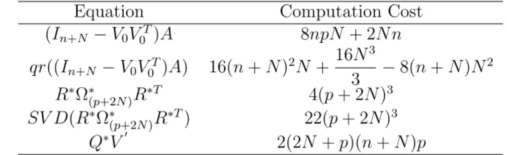
Table 3.1: The Computation cost to update a model with N observations using block updating
Equation Computation Cost (In+N −V0V0T)A 8npN + 2N n qr((In+N −V0V0T)A) 16(n+N)2N+ 16N3 3 −8(n+N)N 2 R∗Ω∗(p+2N)R∗T 4(p+ 2N)3 SV D(R∗Ω∗(p+2N)R∗T) 22(p+ 2N)3 Q∗V0 2(2N +p)(n+N)p
2)(n+ 1) +...+ (8p+ 2)(n+N −1) operations, while performing this step using the proposed block updating uses only (8p+ 2)N n operations.
The steps to calculate the total computation cost of the proposed al-gorithm are as follows: Performing efficient matrix multiplication, the cal-culation of the part of A that is orthogonal to V0 of Equation (3.10) needs
(8p+2)nN operations. Then, performing the QR-decomposition of Equation (3.11) requires 6(n+N)2N+16N3
3 −8(n+N)N
2 operations (Golub & Loan
(1996)). Thereafter, calculation of the product of the three middle matrix of Equation (3.12) would need 4(p+ 2N)3 operations. Then, an application of
a small SVD in the obtained matrix of Equation (3.14) would require only 22(p+ 2N)3 operations. Eventually a rotation of the eigenvector using Equa-tion (3.15) requires 2(2N+p)(n+N)poperations. Adding these numbers of operations, we obtain the total computational cost present in Table 3.1.
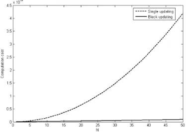
This algorithm allows gain of computation only when a small number of the dominant principal components are updated. Because the amount of computation gain, of using the block updating method instead of using batch updating with SVD or single updating of Hoegaerts et al. (2007), is not clear, Figure 3.1 provides comparisons of the computation cost for different algorithms using different numbers of principal components p.
It is clear from Figure 3.1 that for a reduced number of principal compo-nents (p less than half of n) imply an important reduction in computation cost compared to the SVD method and single updating. Moreover, Figure 3.2 shows that block updating of KPCA reduces computation cost as compared to single updating. However, this gain in computation cost is at the expense of an approximated solution of the eigenvalues and eigenvectors. To analyze
CHAPTER 3. FAST ADAPTIVE KERNEL PRINCIPAL COMPONENTS ANALYSIS
Figure 3.1: Comparison of computation cost for different numbers of principal components p with n equal to 1000 and N equal to 10
Figure 3.2: Computation cost in relation to the size of data block N with n equal to 1000 and p equal to 10
3.3. COMPARISON OF BLOCK UPDATING BASED ON BENCHMARK STUDY
the performance of the proposed algorithm in terms of accuracy next section outlines results obtained using a benchmark data.
3.3
Comparison of block updating based on
benchmark study
In this section, based on a benchmark dataset, we present an analysis of the proposed algorithm in terms of accuracy and speed. The dataset is called Abalone (Blake and Merz, 1998) and it allows predicting the age of abalone from physical measurements. The data set has 4177 instances and 7 exploratory variables. The radial kernel is used with a parameter sigma equal to 5. Because handling the eigenproblem with batch SVD for a 4177×
4177 kernel matrix is difficult, only a set of 3000 observations is used to analyze the different methods. Even though 5 principal components cover more than 90 % of the total variance, as a caution, we select a number of principal components equal to 20, which explain more than 99 % of the total energy. The eigenvector problem starts with an initial model based on training of the first 500 instances and tracking is made by introducing 10 observations into each updating step. In order to compare the speed of different methods to update the KPCA model, Figures 3.3 and 3.4 provide the time needed to update the model when new data are available. The experiment is conducted in a Matlab environment with a computer that has 1.75 GB RAM memory and 2.71 GHz processor. As comparison to batch calculation using standard SVD, the gain of computation time increases as the size of the training data becomes bigger. Also the time needed by block KPCA to update the eigenproblem is more stable than when using batch SVD. As comparison to single updating, we notice that Block SVD is approximately 5 times faster than using single updating. This fact is useful in many applications where the updating procedure needs to be processed with other steps in a short time.
CHAPTER 3. FAST ADAPTIVE KERNEL PRINCIPAL COMPONENTS ANALYSIS
Figure 3.3: Time needed to update the KPCA model using batch SVD and block updating
Figure 3.4: Time needed to update the KPCA model using single updating and block updating
3.3. COMPARISON OF BLOCK UPDATING BASED ON BENCHMARK STUDY
3.3.1
Relative error analysis
In order to assess the performance of the proposed method in terms of ap-proximation accuracy, first, we use an overall measure of accuracy which is the relative error calculated by the distance between the constructed matrix obtained by KPCA model and the original data. This measure is calculated by the matrix Frobenius norm, as follows
RE= K− ˜ K F kKkF , (3.23)
where K is the original matrix and ˜K =VΩpVT is a rank−papproximation
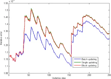
using KPCA model. This measure is computed for different algorithms and comparison of the relative error of the proposed algorithm with that of single updating and batch using SVD is given in Figure 3.5. We notice that the relative errors are approximately the same with a maximal relative error equal to 1.5 10−4. This means that different methods represent relatively well the original data with a good tracking for single updating and block updating.
Figure 3.5: Comparison of reconstruction errors of different updating meth-ods
CHAPTER 3. FAST ADAPTIVE KERNEL PRINCIPAL COMPONENTS ANALYSIS
Another measure of accuracy is the Relative Error between the eigenval-ues computed by batch SVD and those computed using block updating. This indicator is calculated as follows
REλ =
λ−˜λ
λ . (3.24)
whereλ and ˜λ are the eigenvalues computed respectively by SVD and block updating.
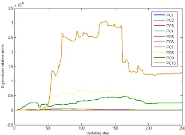
This measure is controlled over 250 iteration steps, for the 10 first dom-inant components. From Figure 3.6 we notice that the domdom-inant principal components are well approximated, with maximal relative errors rate equal to 3.5 10−6 . Also, we note that the accuracy increases for the first principal
components.
Figure 3.6: Relative errors of the first 10 principal components calculated by the difference between eigenvalues obtained by batch SVD and block updat-ing
3.4. CONCLUSION
3.3.2
Orthogonality analysis
In order to test the orthogonality of the obtained principal components using block updating for several iterations, a criterion of the orthogonality of the eigenspace can be calculated by the scalar orthogonality measure, obtained as follows E⊥ = I−VTV 2.
A zero value indicates a perfect orthogonality. During all the updating process, the orthogonality of the KPCA model using block updating is very well-preserved with values of scalar orthogonality measure between 10−8and
10−12. This fact means that the obtained components using block updating of KPCA are, over several iterations, approximately orthogonal.
3.4
Conclusion
This chapter discusses a proposed block updating algorithm for training of the dominant components of KPCA model. The updating method can pro-vide a reduced computation cost in comparison to batch SVD and single updating of Hoegaerts et al (2007). This gain facilitates extension of the use of KPCA method to many machine learning based applications, where fast updating of a large-scale model is required. Analysis of the accuracy and stability of the proposed updating method shows that it provides a good tracking of the original matrix with a small reconstruction error. Also in com-parison to batch KPCA, the proposed algorithm has a good approximation of the eigenvalues with a good preservation of eigenvectors orthogonality.
4
Assessment of the proposed chart
using benchmark studies
An issue concerning the proposed adaptive monitoring technique is to eval-uate it with respect to other PCA process control strategies. We propose to compare performance of Adaptive window Kernel Principal (AKPCA) with Moving Window KPCA (MWKPCA) and Adaptive PCA (APCA). APCA is based on linear PCA and MWKPCA is based on KPCA model. In contrast to the proposed AKPCA control chart, APCA and MWKPCA have fixed model sizes and allow handling of a single observation at a time. Section 1 provides the way to tune control chart parameters. Section 2 investigates performances of different charts using a simulated multivariate nonlinear pro-cess. Section 3 applies the developed charts to monitor a complex industrial chemical process called Tennessee Eastman (TE) process. Section 4 provides the conclusion of this chapter.
4.1
Parameters selection
In order to implement the different control charts, several parameters need to be tuned. These parameters are the sigma of the radial kernel function, the number of Principal Components (PCs), the risk level of the control charts and the size of the initial PCA models.
First of all, for KPCA based charts, the valueσ of the radial kernel func-tion is tuned based on the method of Park and Park (2005), which proposes to select σ =C·Averd, where Averd is the mean distance between all ob-servations in feature space and C is a predetermined value. In this study,
CHAPTER 4. ASSESSMENT OF THE PROPOSED CHART USING BENCHMARK STUDIES
the C value is set to be equal to the square root of the number of process variables. To select the number of PCs, this study uses two of the most used procedures named cross-validation and Cumulative percent variance. The first technique divides the dataset into a training dataset that allows obtain-ing the eigenproblem solution and a test dataset that allows calculatobtain-ing the reconstruction error of the PCA model. The number of PCs which provides most contribution to the minimization of the reconstruction error is selected. The cross-validation procedure is more adequate to select the number of PCs for Q control chart because this statistic allows monitoring of the reconstruc-tion error. However, the Cumulative percent variance procedure selects the p first eigenvalues that capture 95 % of the total variance. This procedure is used to select the number of PCs for T2 control chart since this statistic
mea-sures the distance obtained by projecting observations to the most important PCs. The values ofαlevels of T2 andQbased control charts are set in a way
to provide approximately equally small false alarm rates. Concerning the size of the initial PCA models and the size of the sample used to calculate the initial control chart limits, while Li et al. (2000) used 22 % of the data, Liu et al. (2009) used 30 % of the available data to train and calculate initial PCA models and control charts limits. Also in this study, for each process, 30% of the data is used for construction of the different control charts, such that 20 % of the available sample is used to train initial PCA models and 10 % to calculate initial control limits. For AKPCA chart, the size of the window can vary between 80 % and 120 % of the initial KPCA model size.
Evaluation of different control strategies is given by reporting the degree of accuracy of each method in detecting the true out-of-control situations and avoiding false alarms. Performance evaluation of the accuracy can be reported by using the false alarm rate (Type I error rate) and the detection rate criterion. The first statistic gives information about the robustness of the adopted method against normal system changes whilst the second statistic gives information about the sensitivity and efficiency of detecting faults.
In order to assess different control strategies, we use two simulated bench-mark case studies. The first simulated process is a nonlinear multivariate non-stationary system and the second process is named Tennesee Eastman process which contains 41 state variables that exhibit several nonlinear dy-namics and multistage phases. The description of these processes as well as performances of different control charts are presented in next sections.
4.2. MULTIVARIATE NONLINEAR SIMULATED PROCESS
4.2
Multivariate nonlinear simulated process
The simulated multivariate nonlinear process is described as follows (Zhang and Yang (2000)): y1 = 0.5t2−2t+ 0.5 +ζ y2 =t2+t+ sin(πt) +ζ y3 = 2t2−t−2 cos(πt) +ζ (4.1)where ζ is a random noise and t∈[−1,1].
An illustration of the simulated process is shown in Figure 4.1. In this study, 20 normal samples, each containing 500 observations, are generated. To test the detection performance of the different procedures, this study sim-ulates 7 faults introduced after observation 200. These faults are presented in Table 4.1.
Figure 4.1: Illustration of the simulated multivariate nonlinear process
For Q and T2 based APCA control charts, 2 PCs are selected based on the cross-validation method and the Cumulative percent variance. This value contributes to more than 95 % in the minimization of the reconstruction er-ror and explains more than 95 % of the total variance. For KPCA based models, the value of sigma is set to 5 and the number of PCs is set to
CHAPTER 4. ASSESSMENT OF THE PROPOSED CHART USING BENCHMARK STUDIES
Table 4.1: List of the simulated faults for the multivariate nonlinear process
Fault Description
1 Increase of y1 by 0.02k.(k is the sample number) 2 Increase of y2 by 0.02k.
3 Add to y3 a random effect N(0,1).
4 y1 =y1+ 2t;y2 =y2+ 0.02k. (t is the time index) 5 y1 =y1+N(0,1);y3 =y3 + 2t2.
6 y2 =y2+ 0.02k.;y3 =y3+ 2t.
7 y1 =y1+ 2t;y2 =y2+ 0.02k;y3 =y3+ 2t.
10 for Q control chart and 4 for T2 control chart. Introduction of
obser-vations into the AKPCA model is made by blocks of 5. First, in order to show that Batch PCA and KPCA models are not appropriate to monitor of non-stationary processes, Figure 4.2 shows monitoring performances of both methods when the process is operating under normal condition. The false alarm rate provided by Batch PCA and Batch KPCA are respectively 48 % and 90 %. Therefore analysis of the detection performance of these meth-ods is not performed, since these control charts are not adequate to monitor non-stationary processes. However, as shown in Figure 4.3 and in contrast to the fixed models, applying adaptive PCA based control charts to the same data set, allows better capabilities of adaptation to nonlinear non-stationary behaviour of the process. It should be noted that the control limitsQlimitand
Tlimitof the different adaptive charts are slightly variable over time due to the
fact that they are calculated recursively as described in Section 4. This fact allows a better adaptation to the condition in which the process is operating. To analyze detection capabilities for the different adaptive procedures, mon-itoring performances of APCA, MWKPCA and AKPCA are summarized in Table 4.2.
First, we notice that Q based adaptive charts have overall better fault detection capabilities than T2 based control charts, especially for Kernel
based procedures. This result confirms the analysis of Lee et al. (2004) which states that T2 of KPCA is less reliable than Q chart. Moreover, detection rates of AKPCA are higher than that of APCA and MWKPCA control charts. As an example, when Fault 4 is introduced APCA (Q), MWKPCA (Q) and AKPCA (Q) detects respectively on average 59 %, 45 % and 96 %, of the total faults. Therefore, this result confirms that AKPCA is more
4.2. MULTIVARIATE NONLINEAR SIMULATED PROCESS
Figure 4.2: Batch PCA and KPCA monitoring charts in the case of normal operating condition. The blue and red lines represent respectively the value of the control statistic and its limit
CHAPTER 4. ASSESSMENT OF THE PROPOSED CHART USING BENCHMARK STUDIES
Figure 4.3: Adaptive PCA and KPCA based monitoring charts in the case of normal operating condition
CHAPTER 4. ASSESSMENT OF THE PROPOSED CHART USING BENCHMARK STUDIES
Figure 4.4: Adaptive PCA and KPCA based monitoring charts in the case of Fault 4, where the fault starts after observation 100
4.3. TENNESSEE EASTMAN PROCESS
robust in detecting disturbances. This can be explained by the fact that AKPCA model does not update the model after one observation but after a block of data is tested. Thus, the model has a better ability to overcome contamination by out-of-control observations. This fact can be observed in Figure 4.4, where APCA (Q) and MWKPCA (Q) charts first detect the fault, but after testing and introducing certain observations into the models, detection of this fault is not more possible since it is assimilated as a normal operating change. Moreover, the extreme frequency of updating APCA and MWKPCA models, which is made after each new observation, can imply a decrease in the sensitivity to smaller shifts. In contrast, block AKPAC allows a small delay for updating which can improve detection of this kind of shifts.
Table 4.2: Monitoring results of APCA, MWKPCA and AKPCA charts for several faults
APCA MWKPCA AKPCA
T2 Q T2 Q T2 Q
False alarm rate 0.02 0.02 0.03 0.02 0.03 0.02 Detection rate Fault 1 0.62 0.76 0.08 0.41 0.54 0.99 Fault 2 0.31 0.56 0.06 0.43 0.44 0.99 Fault 3 0.02 0.01 0.07 0.01 0.05 0.09 Fault 4 0.53 0.59 0.10 0.45 0.40 0.96 Fault 5 0.02 0.02 0.10 0.03 0.10 0.01 Fault 6 0.37 0.46 0.05 0.30 0.42 0.94 Fault 7 0.52 0.73 0.10 0.42 0.41 0.98 Mean Detection 0.34 0.45 0.08 0.29 0.34 0.71
4.3
Tennessee Eastman process
The Tennessee Eastman (TE) process is a benchmark simulation model of a complex industrial chemical process proposed by Downs and Vogel (1993). The system contains five major units: a reactor, a condenser, a recycle com-pressor, a separator, and a stripper. The process has 41 state variables that