Testing independence based on Bernstein empirical copula and copula density.

(1)

Durham Research Online

Deposited in DRO: 02 November 2016

Version of attached le: Accepted Version

Peer-review status of attached le: Peer-reviewed

Citation for published item:

Belalia, M. and Bouezmarni, T. and Lemyre, F.C. and Taamouti, A. (2017) 'Testing independence based on Bernstein empirical copula and copula density.', Journal of nonparametric statistics., 29 (2). pp. 346-380. Further information on publisher's website:

https://doi.org/10.1080/10485252.2017.1303063

Publisher's copyright statement:

This is an Accepted Manuscript of an article published by Taylor Francis Group in Journal of Nonparametric Statistics on 23/03/2017, available online at: http://www.tandfonline.com/10.1080/10485252.2017.1303063.

Additional information:

Use policy

The full-text may be used and/or reproduced, and given to third parties in any format or medium, without prior permission or charge, for personal research or study, educational, or not-for-prot purposes provided that:

• a full bibliographic reference is made to the original source

• alinkis made to the metadata record in DRO

• the full-text is not changed in any way

The full-text must not be sold in any format or medium without the formal permission of the copyright holders. Please consult thefull DRO policyfor further details.

(2)

October24,2016

Testing Independence Based on Bernstein Empirical Copula and

Copula Density

M. Belaliaa, T. Bouezmarnia∗, F.C. Lemyre aand A. Taamouti b

a_D´_{epartement de math´}_{ematiques, Universit´}_{e de Sherbrooke, Canada;}b_{Durham University} Business School, UK

In this paper we provide three nonparametric tests of independence between continuous random variables based on the Bernstein copula distribution function and the Bernstein copula density function. The first test is constructed based on a Cram´er-von Mises divergence-type functional based on the empirical Bernstein copula process. The two other tests are based on the Bernstein copula density and use Cram´er-von Mises and Kullback-Leibler divergence-type functionals, respectively. Furthermore, we study the asymptotic null distribution of each of these test statistics. Finally, we consider a Monte Carlo experiment to investigate the performance of our tests. In particular we examine their size and power which we compare with those of the classical nonparametric tests that are based on the empirical distribution function.

Keywords:Bernstein empirical copula; Copula density; Cram´er–von Mises statistic; Kullback-Leibler divergence-type; Independence test.

1. Introduction

Testing for independence between random variables is important in statistics, economics, finance and other disciplines. In economics, tests of independence are useful to detect possible economic causal effects that can be of great importance for policy-makers. In finance, identifying the dependence between different asset prices (returns) is essential for risk management and portfolio selection. Standard tests of independence are given by the usual T-test and F-test that are defined in the context of linear regression models. However, these tests are only appropriate for testing independence in Gaussian models, thus they might fail to capture nonlinear dependence. With the recent growing interest in nonlinear dependence, it is not surprising that there has been a search for alternative dependence measures and tests of independence. In this paper we propose three nonparametric tests ∗_{Corresponding author. Email: Taoufik.Bouezmarni@USherbrooke.ca}

(3)

of independence. These tests are model-free, hence they can be used to detect both linear and nonlinear dependence.

Nonparametric tests of independence have recently gained momentum. In particular, several statistical procedures have been proposed to test for the independence between two continuous random variables X and Y. Most classical tests of independence were initially based on some measures of dependence such as the Pearson linear correlation coefficient ρ, which takes the value 0 under the null hypothesis of no correlation. Other tests of independence have been constructed using other popular measures of dependence that are based on ranks. The rank-based measures of dependence do not depend on the marginal distributions. The most used rank-based measures are Kendall’s tau and Spear-man’s rho. The independence tests that are based on Kendall’s tau (resp. SpearSpear-man’s rho) were investigated by Prokhorov (2001) (resp. Borkowf (2002)). These tests are usually inconsistent, which means that under some alternatives their power functions do not tend to one as the sample size tend to infinity.

To overcome the inconsistency problem of the above tests,Blum, Kiefer, and Rosenblatt

(1961) were among the first to use nonparametric test statistics based on comparison of em-pirical distribution functions. For bivariate random variablesX andY, Blum et al.(1961) use a Cram´er–von Mises distance to compare the joint empirical distribution function of (X, Y); say Hn(x, y) = 1_nPni=1I(Xi ≤ x, Yi ≤ y), with the product of its corresponding

marginal empirical distributions, i.e., Fn(x) = Hn(x,∞) and Gn(y) = Hn(∞, y).

There-after, other researchers have considered using empirical characteristic functions; for review see Feuerverger(1993) andBilodeau and Lafaye de Micheaux(2005), among others.

When the marginal distributions of a random vector X= (X1, ...., Xd) are continuous,

Sklar(1959) has shown that there exists a unique distribution functionC[hereafter copula function] with uniform marginal distributions, such as

H(x1, ...., xd) =C(F1(x1), ..., Fd(xd)),

for x1, ..., xd ∈ Rd.1 Under the null hypothesis of independence between the components of X, the copula function is equal to the independent copula Cπ, which is defined as

Cπ(u) =Cπ(u1, ..., ud) =Qdj=1uj, foru∈[0,1]d, i.e., H0:C(u) =Cπ(u)≡ d Y j=1 uj, for u∈[0,1]d. (1)

The tests based on the distribution and characteristic functions discussed above have inspired Dugué(1975),Deheuvels (1981a,b,c),Ghoudi, Kulperger, and Rémillard (2001), and Genest and Rémillard (2004) to construct tests of mutual independence between the

(4)

components ofXbased on the observationsXi = (Xi,1, ...., Xi,d), fori = 1, .., n,and using

the test statistic

Sn = Z [0,1]d n    Cn(u)− d Y j=1 uj    2 du, (2)

where Cn(u) is the empirical copula originally proposed by Deheuvels(1979) and defined

as Cn(u) = 1 n n X i=1 d Y j=1 I{Vi;j ≤uj}, foru= (u1, ..., ud)∈[0,1]d, (3)

where I{.} is an indicator function and Vi;j = Fj;n(Xi,j), for j = 1, ..., d, with Fj;n(.) is

the empirical cumulative distribution function of the component Xi,j,for i= 1, . . . , n. An

interesting aspect of the above test statistic is that, under the null of mutual independence, the empirical processCn(u) =

√

n(Cn(u)−Cπ(u)) can be decomposed, using the M¨obius

transform, into 2d ₋_d₋_{1 sub-processes} √_nM

A(Cn), for A ⊆ {1, ..., d} and |A| > 1,

that converge jointly to tight centred mutually independent Gaussian processes; seeBlum et al. (1961),Rota(1964) andGenest and R´emillard(2004). However, this test fails when the dependence happens only at the tails. For example, as we will see in Section 5, when the data are generated from Student copula with Kendall’s tau equal to 0 and degree of freedom equal to 2, the power of the test which is based on the empirical copula is low. This indicates that the empirical copula-based test is not able to detect tail dependence. In general, this test does not perform well in term of power in the presence of weak dependencies.

In this paper, we propose several nonparametric copula-based tests for independence that are easy to implement and provide a better power compared to the empirical copula-based test. The first test is a Cram´er-von Mises-type test that we construct using Bernstein empirical copula. Bernstein empirical copula was first studied by Sancetta and Satchell

(2004) for i.i.d. data, who showed that, under some regularity conditions, any copula function can be approximated by a Bernstein copula. Recently, Janssen, Swanepoel, and Veraverbeke(2012) have shown that the Bernstein empirical copula outperforms the clas-sical empirical copula estimator. This latter result has motivated us to use the Bernstein copula function, instead of the standard empirical copula, for testing the null hypothesis in (1). For weak dependencies, our results show that the test based on Bernstein empirical copula outperforms the empirical copula-based test. However, the two tests fail in term of power when the null hypothesis is for example a Student copula with zero Kendall’s tau and small degree of freedom. The difficulty of distinguishing between the independent cop-ula and Student copcop-ula with zero Kendall’s tau and small degree of freedom, illustrated in Figure 1and discussed in Section3.2, may explain the low power of nonparametric copula

(5)

distribution-based tests.

To overcome the above problem, we introduce two other nonparametric tests based on Bernstein empirical copula density.Bouezmarni, Rombouts, and Taamouti(2010) have studied the Bernstein copula density estimator and derived its asymptotic properties under dependent data. These properties have recently been reinvestigated inJanssen, Swanepoel, and Veraverbeke(2014). The motivation for using Bernstein copula density in the construc-tion of our tests is illustrated in Figure 1, which shows that the copula density is flexible in terms of detecting the independence between the variables of interest. In particular, the shape of the copula density changes according to the type and degree of dependen-cies. Thus, our second test is a Cram´er-von Mises-type test which is defined in terms of Bernstein copula density estimator. The third test that we propose is based on Kullback-Leibler divergence which is originally defined in terms of probability density functions. This divergence can be rewritten in terms of copula density, see Blumentritt and Schmid

(2012). Consequently, the third test is a Kullback-Leibler divergence-type test that we construct based on Bernstein copula density estimator. Our results show that these two tests outperform both the Bernstein copula and empirical copula-based tests, and are able to detect the weak dependencies and the dependence that happens at the extreme regions of the Student copula.

Furthermore, we establish the asymptotic distribution of each of these tests under the null hypothesis of independence, and we show their consistency under a fixed alternative. Finally, we run a Monte Carlo experiment to investigate the performance of these tests. In particular, we examine and compare their empirical size and power to those of non-parametric test which is based on the empirical copula process considered in Deheuvels

(1981c),Genest, Quessy, and R´emillard (2006), andKojadinovic and Holmes (2009). The remainder of the paper is organized as follows. In Section 2, we provide the defini-tion of Bernstein copula distribudefini-tion and its properties. Thereafter, we define the process of Bernstein copula {Bk,n(u) :u∈[0,1]d}that we use to construct our first test of

inde-pendence. In Section 3, we define the Bernstein copula density that we use to build our second test of independence based on Cram´er-von Mises divergence. Section 4is devoted to our third nonparametric test of independence that we construct based on Kullback-Liebler divergence which we define in terms of Bernstein copula density. We establish the asymptotic distribution of each of these test statistics under the null, and we show their consistency under a fixed alternative. Section 5reports the results of a Monte Carlo sim-ulation study to illustrate the performance (empirical size and power) of the proposed test statistics. We conclude in Section 6. The proofs of main theoretical results and some technical computations are presented in Appendix AandB, respectively.

(6)

2. Test of independence using Bernstein copula 2.1. Bernstein copula distribution

In this section, we define the estimator of Bernstein copula distribution and we discuss its asymptotic properties. This estimator will be used to build the first test of indepen-dence.Sancetta and Satchell(2004) were the first to apply a Bernstein polynomial for the estimation of copulas. The Bernstein copula estimator is given by

Ck,n(u) = k X v1=0 ... k X vd=0 Cn _v 1 k , ..., vd k d Y j=1 Pvj,k(uj), for u= (u1, ..., ud)∈[0,1] d , (4)

where Cn(.) is the empirical copula defined in Equation (3),Pvj,k(.) is the binomial

prob-ability mass function with parameters vj and k, and k is an integer that represents a

bandwidth parameter and depends on the sample sizen. Janssen et al.(2012) have stud-ied the asymptotic properties (almost sure consistency and asymptotic normality) of the estimator in (4). In particular, they provided its asymptotic bias and variance and showed that this estimator outperforms the empirical copula in terms of mean squared error.

We now define the following empirical Bernstein copula process under the null hypothesis of independence:

Bk,n(u) =n1/2{Ck,n(u)−Cπ(u)}, for u∈[0,1]d, (5)

where Cπ(u) is the independent copula function defined in Equation (1). The following

Lemma from Janssen et al. (2012) states the weak convergence of the processBk,n under

H0 in (1). It will be used to establish the asymptotic distribution of our first test of independence presented in Section2.2.

Lemma 1 (Janssen et al. (2012)) Suppose that k→ ∞ asn→ ∞. Then, under H0, the

process Bk,n converges weakly to Gaussian process, Cπ(u), with mean zero and covariance

function given by:

E      I(U1 ≤u1, ..., Ud ≤ud)−Cπ(u)− d X j=1 Cπj(u){I(Uj ≤uj)−uj}    ×    I(U1≤v1, ..., Ud ≤vd)−Cπ(v)− d X j=1 Cπj(v){I(Uj ≤vj)−vj}     ,

where Uj, for j = 1, . . . , d, are i.i.d. U[0,1], Cπj(u) = Qi6=jui, and I(.) is an indicator function.

(7)

2.2. Test of independence

The empirical Bernstein copula process in (5) will be used to construct the test statis-tic of our first nonparametric test of independence. For a given sample {X1, . . . ,Xn}, a convenient way for testing H0 in (1) is by measuring the distance between the Bernstein empirical copula Ck,n(u) and the independent copula function Cπ in (1). This distance

can be measured using a Cram´er–von Mises divergence that leads to the following test statistic: Tn =n Z [0,1]d  Ck,n(u)− d Y j=1 uj   2 du=n Z [0,1]dB 2 k,n(u)du. (6)

Other test statistics can be obtained using different criteria such as the one used in Kolmogorov-Smirnov test statistic. We can also consider integrating with respect to the Lebesgue-Steiltjes measure dCn(u), but under the null hypothesis H0 this should lead to similar result as the test statistic in Equation (6). The following proposition provides an explicit expression for the test statistic Tn in (6) [see the proof of Proposition 1 in

Appendix A]. Proposition 1 If we note k X v1=0 . . . k X vd=0 k X s1=0 . . . k X sd=0 = X (v,s) , then Tn =n X (v,s) Cn _v 1 k, ..., vd k Cn _s 1 k , ..., sd k d Y j=1 k vj k sj β(vj+sj+ 1,2k−vj−sj+ 1) −2n k X v1=0 ... k X vd=0 Cn _v 1 k , ..., vd k d Y j=1 k vj β(vj+ 2, k−vj+ 1) + n 3d,

whereβ(., .)is the beta function which is defined as β(w1, w2) = 1 R 0

tw1−1₍₁₋_t₎w2−1

dt,for

w1 and w2 two positive integers.

The next result that follows from Lemma1and the continuous mapping theorem estab-lishes the asymptotic distribution of test statistic Tn.

Proposition 2 Suppose that k → ∞ as n → ∞. Then, under the null hypothesis of

independenceH0in(1), the test statisticTnin (6) converges in distribution to the following

integral of a Gaussian process:

Z

[0,1]dC

2

π(u)du,

where the process Cπ(u) is defined in Lemma 1.

(8)

rejecting or failing to rejectH0. A Monte Carlo simulation-based approach can also be used to simulate the distribution of the test statisticTnunder the null hypothesisH0.The latter approach consists in generating several samples underH0,i.e., we generate random vectors [0,1]d_{under the null hypothesis of independence and for each of these samples we calculate}

the test statisticTn. Thereafter and for a given significance levelα∈(0,1), we compute the

(1-α)-th empirical quantile of the simulated distribution of the test statisticTn. We then

reject the null hypothesis of independence if the observed test statistic, computed using the observed data, is greater than the calculated (1-α)-th quantile. In finite sample settings, our simulation results suggest that a Monte Carlo-simulation based approach provides a better approximation for the distribution ofTn compared to the asymptotic distribution.

This means that it is better to use critical values (p-values) that are calculated using Monte Carlo simulation instead of the ones that come from the asymptotic distribution.

We next establish the consistency of our first test for a fixed alternative [see the proof of Proposition3 in AppendixA].

Proposition 3 Suppose thatk → ∞asn→ ∞. Then, the test based on the test statistic Tn in (6) is consistent for any bounded copula density c such that

Z  C(u)− d Y j=1 uj   2 du>0.

3. Test of independence using Bernstein copula density

3.1. Bernstein copula density

In this section, we define the estimator of Bernstein copula density that we will use to build our second nonparametric test of independence. Before doing so, let us first recall the definition of copula density using copula distribution. If it exists, the copula density, denoted by c, is defined as follows:

c(u) =∂dC(u)/∂u1...∂ud, (7)

where C is the copula distribution.

Now, from Equation (7) and since the Bernstein copula distribution introduced in Sec-tion 2is absolutely continuous, the Bernstein copula density is defined as follows:

ck(u) = k X v1=0 ... k X vd=0 C _v 1 k , ..., vd k d Y j=1 Pv0j,k(uj),

(9)

to u. Thus, the estimator of Bernstein copula density is given by ck,n(u) = k X v1=0 ... k X vd=0 Cn _v 1 k , ..., vd k d Y j=1 Pv0j,k(uj), (8)

whereCn(.) is the empirical copula distribution. FromBouezmarni et al.(2010), the

Bern-stein copula density estimator can be rewritten as follows:

ck,n(u) = 1 n n X i=1 Kk(u,Vi), foru∈[0,1]d, (9) with Kk(u,Vi) =kd k−1 X ν1=1 ... k−1 X νd=1 I{Vi ∈Ak(ν)} d Y j=1 Pνj,k−1(uj),

where Pνj,k−1(.) is the binomial probability mass function with parameters νj andk−1,

Vi = (F1;n(Xi,1), ..., Fd;n(Xi,d)), with Fj;n(.), for j = 1, ..., d, the empirical distribution

based on Xi,j, fori= 1, . . . , n,andAk(ν) =ν_k1,ν1_k+1×...×

h νd k , νd+1 k i ,withk an integer that plays the role of bandwidth parameter.

The Bernstein copula density estimator in (9) is proposed and investigated inSancetta and Satchell (2004) for i.i.d. data. Later, Bouezmarni et al. (2010) have used a Bern-stein polynomial to estimate the copula density for time series data. They provided the asymptotic bias and variance, uniform a.s. convergence, and asymptotic normality of the estimator of Bernstein copula density for α-mixing data. Recently, Janssen et al.(2014) have reinvestigated this estimator by establishing its asymptotic normality under i.i.d. data.

We will now use the estimator of Bernstein copula density in Equation (9) to define the test statistic of our second nonparametric test of independence. Before doing so, observe that testing the null hypothesis of independence is equivalent to testing

H0 :c(u) = 1, u∈[0,1]d.

To test the above null hypothesis, we consider the following Cram´er–von Mises-type test statistic

In(u) =

Z

[0,1]d

(ck,n(u)−1)2du, (10)

(10)

As mentioned in the introduction, building tests of independence based on Bernstein copula density instead of Bernstein copula distribution is motivated by the fact that the copula density is able to capture the dependence even when the Kendall’s tau coefficient is small or equal to zero. For example, it is straightforward to see that when Kendall’s tau is equal to zero, one can not distinguish between the Student copula distribution and the independent copula. However, it is easier to distinguish between their corresponding copula density functions. For example, if we consider a Student’s probability density function tν+1with the number of degrees of freedom equal to ν = 2 and Kendall’s tau τ, then the lower/upper tail-dependence coefficient of the Student copula density is equal toλ = 2tν+1(−

√

1 +ν√1−τ /√1 +τ). Hence, even if we take Kendall’s tau equal to zero, the tail-dependence coefficient λ will be equal to 0.1816901, thus different from zero. This situation is illustrated in Figure 1 where Kendall’s tau is taken to be equal to zero.

Now, to establish the asymptotic distribution of the test statistic In under the null H0, we need to introduce the following additional term. For any integers v1 and v2 such that 0≤v1, v2 ≤k−1, we define Γk(v1, v2) = Z 1 0 Pv1,k−1(u)Pv2,k−1(u)du (11) = k−1 v1 ! k−1 v2 ! β(v1+v2+ 1,2k−1−v1−v2).

The following proposition provides a practical expression for the test statisticIn in the

bivariate case [see the proof of Proposition4 in AppendixA].

Proposition 4 Using similar notations to those in Proposition 1, the test statistic in

(10) can be rewritten as follows:

In(u) =k4 k−1 X v1,v10=0 v2,v20=0 Υk(v1, v2)Υk(v10, v20)Γk(v1, v01)Γk(v2, v20)−1,

whereΓk(., .)is defined in Equation (11) andΥk(v1, v2) =Cn v1_k+1,v2_k+1

−Cn v_k1,v2_k+1 − Cn v1_k+1,v_k2 +Cn v_k1,v_k2

, with Cn(., .) denotes the empirical copula.

The following theorem provides the asymptotic distribution of the test statisticIn under

H0 [see the proof of Theorem1 in AppendixA].

Theorem 1 Suppose thatk→ ∞ together withn−1/2k3d/4log log2(n)→0when n→ ∞.

(11)

In,k :=nk−d        In−2−dπd/2n−1kd/2 21/2 r n Pk−1 v1,v2=0Γk(v1, v2) 2od₋_k−2d        d −→ N(0,1),

where In and Γk(., .) are defined in Equations (10) and (11), respectively.

The proof of the following Corollary can be found in Appendix A.

Corollary 1 Suppose that the assumptions of Theorem 1 are satisfied. Then, there

exists a constant R >0such that

nk−d/4 ( In−2−dπd/2n−1kd/2 Rd√₂ ) d −→ N(0,1),

where In is defined in Equation (10).

As for our first test, our simulation results suggest that it is better to use a Monte Carlo simulation-based approach, instead of the asymptotic distribution, for the calculation of critical values (p-values) of the test statisticIn. A brief description of Monte Carlo

simula-tion approach can be found at the end of Secsimula-tion2.2. We next establish the consistency of our second test based on the test statistic In [see the proof of Proposition 5 in Appendix

A].

Proposition 5 Assume that k → ∞ together with n−1/2k3d/4log log2(n) → 0 when n→ ∞. Then, the test based on the test statistic In in (10) is consistent for any bounded

copula density c such that

Z

(c(u)−1)2 du>0.

4. Test of independence based on Kullback-Leibler divergence

4.1. Measure of dependence

Relative entropy, also known as the Kullback-Leibler divergence, is a measure of multivari-ate association which is originally defined in terms of probability density functions. Fol-lowing Blumentritt and Schmid(2012), we rewrite the Kullback-Leibler measure in terms of copula density to disentangle the dependence structure from the marginal distributions.

Blumentritt and Schmid (2012) propose an estimator for Kullback-Leibler measure of de-pendence using the Bernstein copula density estimator. Since the latter is guaranteed to be non-negative, this helps avoid having negative values inside the logarithmic function of the Kullback-Leibler distance. Furthermore, there is no boundary bias problem when we

(12)

use the Bernstein copula density estimator because by smoothing with beta densities this estimator does not assign weights outside its support.

We now review the theoretical aspects of the above measure. Joe et al. (1987), Joe

(1989a), and Joe (1989b) have introduced relative entropy as a measure of multivariate association for the random vector X. The relative entropy is defined as

δ(c) = Z Rd log " f(x) Qd i=1fi(xi) # f(x) dx, (12)

where f is the joint probability density of X and fi is the marginal probability density

of its component Xi, fori= 1, ..., d. According to Sklar (1959), the density function ofX

can be expressed as f(x1, ..., xd) =c(F1(x1), ..., Fd(xd)) d Y i=1 fi(xi), (13)

wherecis the density copula function. Using Equation (13), we can show that the relative entropy in (12) can be rewritten in terms of copula density as

δ(c)≡δ(c) =

Z

[0,1]d

log [c(u)]c(u) du. (14)

The measure δ(c) does not depend on the marginal distributions of X, but only on the copula density c. We will next define a nonparametric estimator of δ(c) that we will use to construct the test statistic of our third test of independence, and we will establish its asymptotic normality.

We have shown that the Kullback-Leibler measure of dependenceδ(c) can be expressed in terms of copula density function c. Thus, an estimator of that measure can be obtained by replacing the unknown copula density c by its Bernstein copula density estimator in Equation (9):

δn(c) =

Z

[0,1]d

log [ck,n(u)]ck,n(u)du. (15)

whereck,n(u) is the Bernstein copula density estimator defined in Equation (9). In practice,

we suggest to replaceck,n(u)duinδn(c) by dCn(u), i.e., to use the following test statistic:

˜ δn(c) = Z [0,1]dlog [ck,n(u)]dCn(u) (16) = 1 n n X i=1 log [ck,n(Vi)].

(13)

Now, observe that the null hypothesis of independence is equivalent to the nullity of the measure δ(c). Thus, our third nonparametric test of independence is based on δn(c). In

other words, we use δn(c) in Equation (15) as a test statistic to test the null hypothesis

H0. The following theorem provides the asymptotic normality of the test statistic δn(c)

[see the proof of Theorem 2in Appendix A].

Theorem 2 Suppose that the assumptions of Theorem 1 are satisfied. Then, underH0,

we have nk−d        2δn(c)−2−dπd/2n−1kd/2 21/2 r n Pk−1 v1,v2=0Γk(v1, v2) 2od₋_k−2d        d −→ N(0,1),

where Γk(., .) and δn(c) are defined in (11) and (15), respectively.

The result in Theorem 2remains unchanged when we replace δn(c) by ˜δn(c) in (16).

As for the test statistics Tn and In, our simulation results suggest that it is better to

use a Monte Carlo simulation-based approach, instead of the asymptotic distribution, for the calculation of critical values (p-values) of the test statistic δn(c). A brief description

of Monte Carlo simulation approach can be found at the end of Section 2.2. Furthermore, the consistency of the test based on δn(c) can be established under the same conditions

as the ones we needed for the consistency of In, using similar arguments as in the proof

of Proposition5.

5. Simulation studies

We run a Monte Carlo experiment to investigate the performance of nonparametric tests of independence proposed in the previous sections. In particular, we study the power of the test statistics Tn, In and δn using different samples sizes: n= 100, 200, 400, 500. To

calculate the critical values of these test statistics under the null and at 5% significance level, we simulate independent data using the independent copula. Thereafter, we evaluate the empirical power of our tests using different copula functions that generate data under different degrees of dependence following different values of Kendall’s tau coefficientτ = 0, 0.1, 0.25. For Kendall’s τ coefficient greater than 0.5, all the tests provide good and comparable results. The copulas under consideration are Normal, Student, Clayton and Gumbel copulas. Moreover, we compare the power functions of our tests to the power function of the following classical test which is based on the empirical copula process considered in Deheuvels (1981c), Genest, Quessy, and R´emillard (2006), and Kojadinovic

(14)

and Holmes (2009):

Sn =n

Z

[0,1]2

{Cn(u1, u2)−Cπ(u1, u2)}2du1du2. (17) The test statistics Tn, In andδn depend on the bandwidth parameterk which is needed

to estimate the copula density (distribution). We take various values ofkto investigate the sensitivity of the power functions of our nonparametric tests to the bandwidth parameter. A practical bandwidth can be selected using a similar approach to the one proposed by

Omelka, Gijbels, and Veraverbeke (2009) for kernel-based copula estimation, but this is not investigated in this paper and left for future research.Omelka et al.(2009)’s approach involves an Edgeworth expansion of the asymptotic distribution of the test statistics. Finally, we use Monte-Carlo approximations, based on 1000 replications, to compute the critical values and the empirical power of all the tests,Sn, Tn, In andδn.

In the simulations, we consider two scenarios for the marginal distributions used to compute the test statistics. In the first one, we assume that the marginal distributions are known and given by a uniform distribution. In the second scenario, we consider that the marginal distributions are estimated. In the latter scenario we consider different models for the marginal distributions: uniform, normal and Student. Simulation results for the empirical power of the tests that are based on the statisticsTn, In,δn,andSn are reported

in Tables1-3for the first scenario and in Tables4-6for the second scenario. We only provide the results for normal marginals as the results for other distributions are quite similar.

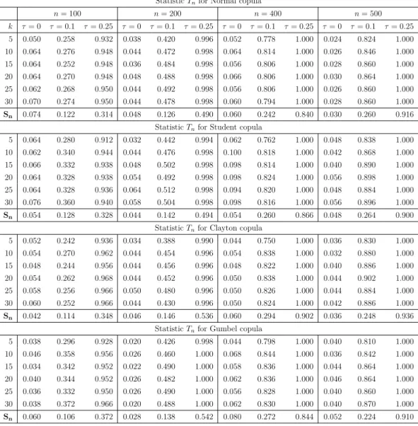
Table 1 compares the power function of our first nonparametric test which is based on the Bernstein copula distribution Tn to the power function of the classical test which is

based on the empirical copula Sn. The simulation results for different copulas, samples

sizes, and degrees of dependence show that both tests provide good empirical size. The power of the two tests increases with sample size and degree of dependence measured by Kendall’s tau. Furthermore, the power functions of both tests are comparable for moderate degree of dependency, but the test based on the Bernstein copula dominates the one based on the empirical copula when Kendall’s tau is small. Finally, the two tests fail in terms of power in the case of Student copula with Kendall’s tau equal to zero. Recall that in the case of Student copula, Kendall’s tau equal to zero does not imply independence, because the dependence may happen in the tail regions.

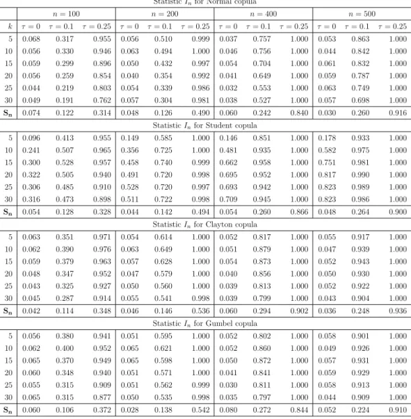
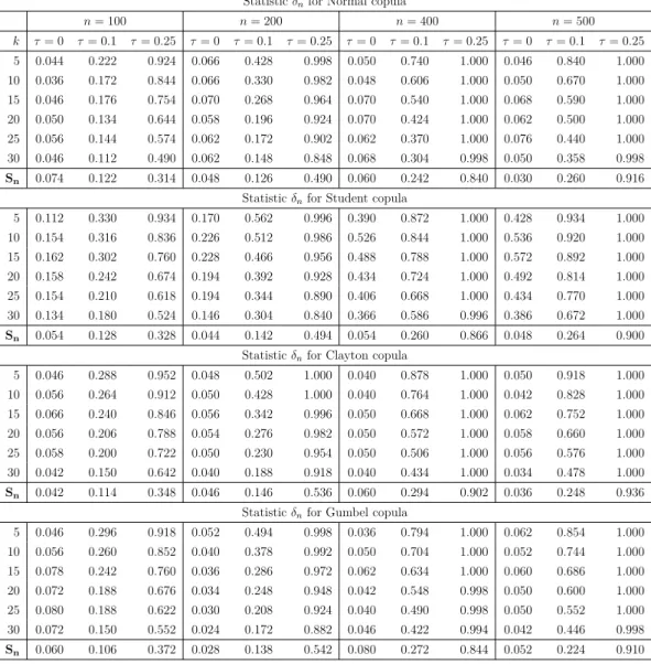
Tables 2 and 3 provide the empirical size and power of nonparametric tests that are based on the test statistics In andδn, respectively. From these, we see that the two tests

generally control the size. Their powers increase with the sample size and the strength of dependence. Compared to the empirical copula-based test Sn, we find that these tests

do much better in terms of power, especially in the case of Student copula with zero Kendall’s tau. For example, when n = 500 and k = 25 the powers of In and δn tests

(15)

The same remark applies when the degree of dependencies is small. For example, under Clayton copula and when τ = 0.1, k = 25, and n = 400, the powers of In and δn tests

are equal to 0.813 and 0.506, respectively, whereas the power of Sn test is equal to 0.294.

The difference becomes even more important when we increase the sample seize. Finally, we find that the Cram´er-von Mises-type test which is defined in terms of Bernstein copula density generally outperforms the test based on Kullback-Leibler divergence and defined as a function of Bernstein copula density estimator.

Table4 shows the power of the testsTn andSn using estimated marginal distributions.

We observe a significant improvement in the power of the testSn compared to the results

in Table 1. But we still find that the test Tn does better than the test Sn in many cases.

Tables5-6show the power of the testsIn andδn.We see clearly that the testsInandδndo

better than the testSn for Student copula and very low dependence, especially forτ = 0.

However, in many cases the test Sn does better than the tests In and δn when τ = 0.1.

Finally, it seems that the test In does better than the other ones (δn andTn).

6. Conclusion

We provided three different nonparametric tests of independence between continuous ran-dom variables based on estimators of Bernstein copula distribution and Bernstein copula density. The first two tests were constructed using Cram´er-von Mises divergence that we define as a function of the empirical Bernstein copula process and the empirical Bern-stein copula density, respectively. The third test is based on Kullback-Leibler divergence originally defined in terms of probability density functions. We first rewrote the Kullback-Leibler divergence in terms of copula density, see also Blumentritt and Schmid (2012). Thereafter, we constructed the third test using an estimator of Kullback-Leibler divergence defined as a logarithmic function of the estimator of Bernstein copula density. Further-more, we provided the asymptotic distribution of each of these tests under the null, and we established their consistency under a fixed alternative. Finally, we ran a Monte Carlo experiment to investigate the performance of these tests. In particular, we examined and compared their empirical size and power to those of classical nonparametric test which is based on the empirical copula considered in Deheuvels(1981c),Genest et al. (2006), and

(16)

x 0.0 0.2 0.4 0.60.8 1.0 y 0.0 0.2 0.4 0.6 0.8 1.0 v 0.0 0.2 0.4 0.6 0.8 1.0 Student copula x 0.0 0.2 0.4 0.60.8 1.0 y 0.0 0.2 0.4 0.6 0.8 1.0 v 0.0 0.5 1.0 1.5 2.0

Student copula density

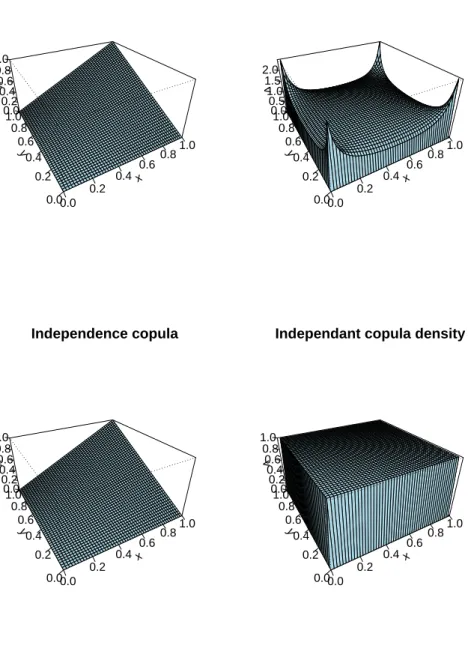
x 0.0 0.2 0.4 0.6 0.81.0 y 0.0 0.2 0.4 0.6 0.8 1.0 v 0.0 0.2 0.4 0.6 0.8 1.0 Independence copula x 0.0 0.2 0.4 0.6 0.81.0 y 0.0 0.2 0.4 0.6 0.8 1.0 v 0.0 0.2 0.4 0.6 0.8 1.0

Independant copula density

Figure 1. This figure compares the student copula distribution (in the top of the left-hand side panel) and the independent copula distribution (in the bottom of the left-hand side panel) and between the student copula density (in the top of the right-hand side panel) and the independent copula density (in the bottom of the right-hand side panel).

(17)

StatisticTnfor Normal copula n= 100 n= 200 n= 400 n= 500 k τ= 0 τ= 0.1 τ= 0.25 τ= 0 τ= 0.1 τ= 0.25 τ= 0 τ= 0.1 τ= 0.25 τ= 0 τ= 0.1 τ= 0.25 5 0.050 0.258 0.932 0.038 0.420 0.996 0.052 0.778 1.000 0.024 0.824 1.000 10 0.064 0.276 0.948 0.044 0.472 0.998 0.064 0.814 1.000 0.026 0.846 1.000 15 0.064 0.252 0.948 0.036 0.484 0.998 0.056 0.806 1.000 0.028 0.860 1.000 20 0.064 0.270 0.948 0.048 0.488 0.998 0.066 0.806 1.000 0.030 0.864 1.000 25 0.062 0.268 0.950 0.044 0.492 0.998 0.056 0.806 1.000 0.026 0.860 1.000 30 0.070 0.274 0.950 0.044 0.478 0.998 0.060 0.794 1.000 0.028 0.860 1.000 Sn 0.074 0.122 0.314 0.048 0.126 0.490 0.060 0.242 0.840 0.030 0.260 0.916 StatisticTnfor Student copula

5 0.064 0.280 0.912 0.032 0.442 0.994 0.062 0.762 1.000 0.048 0.838 1.000 10 0.062 0.340 0.944 0.044 0.476 0.998 0.100 0.818 1.000 0.042 0.868 1.000 15 0.066 0.332 0.938 0.048 0.502 0.998 0.098 0.814 1.000 0.040 0.890 1.000 20 0.064 0.328 0.938 0.054 0.492 0.998 0.098 0.824 1.000 0.056 0.898 1.000 25 0.064 0.328 0.936 0.064 0.512 0.998 0.094 0.820 1.000 0.048 0.884 1.000 30 0.076 0.360 0.940 0.058 0.504 0.998 0.098 0.816 1.000 0.056 0.896 1.000 Sn 0.054 0.128 0.328 0.044 0.142 0.494 0.054 0.260 0.866 0.048 0.264 0.900 StatisticTnfor Clayton copula

5 0.052 0.242 0.936 0.034 0.388 0.990 0.044 0.750 1.000 0.036 0.830 1.000 10 0.054 0.270 0.962 0.044 0.454 0.996 0.054 0.838 1.000 0.032 0.880 1.000 15 0.048 0.244 0.956 0.044 0.456 0.996 0.048 0.822 1.000 0.040 0.886 1.000 20 0.054 0.262 0.968 0.044 0.452 0.996 0.050 0.838 1.000 0.044 0.902 1.000 25 0.058 0.256 0.966 0.050 0.480 0.996 0.050 0.826 1.000 0.044 0.884 1.000 30 0.060 0.252 0.966 0.044 0.430 0.996 0.050 0.824 1.000 0.042 0.886 1.000 Sn 0.042 0.114 0.348 0.046 0.146 0.536 0.060 0.294 0.902 0.036 0.248 0.936 StatisticTnfor Gumbel copula

5 0.038 0.296 0.928 0.020 0.426 0.998 0.044 0.798 1.000 0.040 0.810 1.000 10 0.046 0.358 0.956 0.026 0.460 1.000 0.068 0.844 1.000 0.036 0.842 1.000 15 0.034 0.342 0.952 0.022 0.490 1.000 0.058 0.836 1.000 0.044 0.864 1.000 20 0.040 0.344 0.952 0.026 0.482 1.000 0.062 0.836 1.000 0.046 0.864 1.000 25 0.036 0.332 0.950 0.026 0.490 1.000 0.056 0.828 1.000 0.040 0.860 1.000 30 0.038 0.372 0.966 0.020 0.488 1.000 0.062 0.830 1.000 0.040 0.870 1.000 Sn 0.060 0.106 0.372 0.028 0.138 0.542 0.080 0.272 0.844 0.052 0.224 0.910

Table 1. This table compares the empirical size and power of the test statisticsTnandSnfor different copulas

(Normal, Student, Clayton and Gumbel copulas) with known marginal distributions, different values of Kendall’s tau coefficientτ (τ = 0,0.1,0.25), different sample sizes n(n= 100,200,400,500), and different values for the bandwidthk.

(18)

StatisticInfor Normal copula n= 100 n= 200 n= 400 n= 500 k τ= 0 τ= 0.1 τ= 0.25 τ= 0 τ= 0.1 τ= 0.25 τ= 0 τ= 0.1 τ= 0.25 τ= 0 τ= 0.1 τ= 0.25 5 0.068 0.317 0.955 0.056 0.510 0.999 0.037 0.757 1.000 0.053 0.863 1.000 10 0.056 0.330 0.946 0.063 0.494 1.000 0.046 0.756 1.000 0.044 0.842 1.000 15 0.059 0.299 0.896 0.050 0.432 0.997 0.054 0.704 1.000 0.061 0.832 1.000 20 0.056 0.259 0.854 0.040 0.354 0.992 0.041 0.649 1.000 0.059 0.787 1.000 25 0.044 0.219 0.803 0.054 0.339 0.986 0.032 0.553 1.000 0.063 0.749 1.000 30 0.049 0.191 0.762 0.057 0.304 0.981 0.038 0.527 1.000 0.057 0.698 1.000 Sn 0.074 0.122 0.314 0.048 0.126 0.490 0.060 0.242 0.840 0.030 0.260 0.916 StatisticInfor Student copula

5 0.096 0.413 0.955 0.149 0.585 1.000 0.146 0.851 1.000 0.178 0.933 1.000 10 0.241 0.507 0.965 0.356 0.725 1.000 0.481 0.935 1.000 0.582 0.975 1.000 15 0.300 0.528 0.957 0.458 0.740 0.999 0.662 0.958 1.000 0.751 0.981 1.000 20 0.322 0.505 0.940 0.491 0.720 0.998 0.695 0.952 1.000 0.817 0.990 1.000 25 0.306 0.485 0.910 0.528 0.720 0.997 0.693 0.942 1.000 0.823 0.989 1.000 30 0.316 0.473 0.898 0.511 0.722 0.998 0.709 0.945 1.000 0.823 0.986 1.000 Sn 0.054 0.128 0.328 0.044 0.142 0.494 0.054 0.260 0.866 0.048 0.264 0.900 StatisticInfor Clayton copula

5 0.063 0.351 0.971 0.054 0.614 1.000 0.052 0.817 1.000 0.055 0.917 1.000 10 0.062 0.390 0.976 0.063 0.649 1.000 0.051 0.879 1.000 0.047 0.939 1.000 15 0.059 0.379 0.963 0.057 0.628 1.000 0.054 0.873 1.000 0.052 0.943 1.000 20 0.048 0.347 0.952 0.047 0.579 1.000 0.040 0.856 1.000 0.050 0.930 1.000 25 0.043 0.325 0.927 0.050 0.560 1.000 0.039 0.813 1.000 0.052 0.922 1.000 30 0.045 0.287 0.914 0.055 0.541 0.998 0.039 0.799 1.000 0.043 0.904 1.000 Sn 0.042 0.114 0.348 0.046 0.146 0.536 0.060 0.294 0.902 0.036 0.248 0.936 StatisticInfor Gumbel copula

5 0.056 0.380 0.941 0.051 0.595 1.000 0.052 0.802 1.000 0.058 0.901 1.000 10 0.062 0.400 0.952 0.065 0.621 1.000 0.052 0.860 1.000 0.049 0.926 1.000 15 0.065 0.370 0.949 0.065 0.598 1.000 0.050 0.872 1.000 0.057 0.931 1.000 20 0.060 0.348 0.940 0.051 0.571 1.000 0.041 0.841 1.000 0.059 0.929 1.000 25 0.055 0.315 0.909 0.051 0.562 0.999 0.030 0.811 1.000 0.058 0.913 1.000 30 0.065 0.315 0.877 0.050 0.535 0.998 0.035 0.797 1.000 0.044 0.909 1.000 Sn 0.060 0.106 0.372 0.028 0.138 0.542 0.080 0.272 0.844 0.052 0.224 0.910

Table 2. This table compares the empirical size and power of the test statisticsInandSnfor different copulas

(Normal, Student, Clayton and Gumbel copulas) with known marginal distributions, different values of Kendall’s tau coefficient τ (τ= 0,0.1,0.25) , different sample sizesn(n= 100,200,400,500), and different values for the bandwidthk.

(19)

Statisticδnfor Normal copula n= 100 n= 200 n= 400 n= 500 k τ= 0 τ= 0.1 τ= 0.25 τ= 0 τ= 0.1 τ= 0.25 τ= 0 τ= 0.1 τ= 0.25 τ= 0 τ= 0.1 τ= 0.25 5 0.044 0.222 0.924 0.066 0.428 0.998 0.050 0.740 1.000 0.046 0.840 1.000 10 0.036 0.172 0.844 0.066 0.330 0.982 0.048 0.606 1.000 0.050 0.670 1.000 15 0.046 0.176 0.754 0.070 0.268 0.964 0.070 0.540 1.000 0.068 0.590 1.000 20 0.050 0.134 0.644 0.058 0.196 0.924 0.070 0.424 1.000 0.062 0.500 1.000 25 0.056 0.144 0.574 0.062 0.172 0.902 0.062 0.370 1.000 0.076 0.440 1.000 30 0.046 0.112 0.490 0.062 0.148 0.848 0.068 0.304 0.998 0.050 0.358 0.998 Sn 0.074 0.122 0.314 0.048 0.126 0.490 0.060 0.242 0.840 0.030 0.260 0.916 Statisticδnfor Student copula

5 0.112 0.330 0.934 0.170 0.562 0.996 0.390 0.872 1.000 0.428 0.934 1.000 10 0.154 0.316 0.836 0.226 0.512 0.986 0.526 0.844 1.000 0.536 0.920 1.000 15 0.162 0.302 0.760 0.228 0.466 0.956 0.488 0.788 1.000 0.572 0.892 1.000 20 0.158 0.242 0.674 0.194 0.392 0.928 0.434 0.724 1.000 0.492 0.814 1.000 25 0.154 0.210 0.618 0.194 0.344 0.890 0.406 0.668 1.000 0.434 0.770 1.000 30 0.134 0.180 0.524 0.146 0.304 0.840 0.366 0.586 0.996 0.386 0.672 1.000 Sn 0.054 0.128 0.328 0.044 0.142 0.494 0.054 0.260 0.866 0.048 0.264 0.900 Statisticδnfor Clayton copula

5 0.046 0.288 0.952 0.048 0.502 1.000 0.040 0.878 1.000 0.050 0.918 1.000 10 0.056 0.264 0.912 0.050 0.428 1.000 0.040 0.764 1.000 0.042 0.828 1.000 15 0.066 0.240 0.846 0.056 0.342 0.996 0.050 0.668 1.000 0.062 0.752 1.000 20 0.056 0.206 0.788 0.054 0.276 0.982 0.050 0.572 1.000 0.058 0.660 1.000 25 0.058 0.200 0.722 0.050 0.230 0.954 0.050 0.506 1.000 0.056 0.576 1.000 30 0.042 0.150 0.642 0.040 0.188 0.918 0.040 0.434 1.000 0.034 0.478 1.000 Sn 0.042 0.114 0.348 0.046 0.146 0.536 0.060 0.294 0.902 0.036 0.248 0.936 Statisticδnfor Gumbel copula

5 0.046 0.296 0.918 0.052 0.494 0.998 0.036 0.794 1.000 0.062 0.854 1.000 10 0.056 0.260 0.852 0.040 0.378 0.992 0.050 0.704 1.000 0.052 0.744 1.000 15 0.078 0.242 0.760 0.036 0.286 0.972 0.062 0.634 1.000 0.060 0.686 1.000 20 0.072 0.188 0.676 0.034 0.248 0.948 0.042 0.548 0.998 0.050 0.600 1.000 25 0.080 0.188 0.622 0.030 0.208 0.924 0.040 0.490 0.998 0.050 0.552 1.000 30 0.072 0.150 0.552 0.024 0.172 0.882 0.046 0.422 0.994 0.042 0.446 0.998 Sn 0.060 0.106 0.372 0.028 0.138 0.542 0.080 0.272 0.844 0.052 0.224 0.910

Table 3. This table compares the empirical size and power of the test statisticsδnandSnfor different copulas

(Normal, Student, Clayton and Gumbel copulas) with known marginal distributions, different values of Kendall’s tau coefficientτ (τ = 0,0.1,0.25), different sample sizes n(n= 100,200,400,500), and different values for the bandwidthk.

(20)

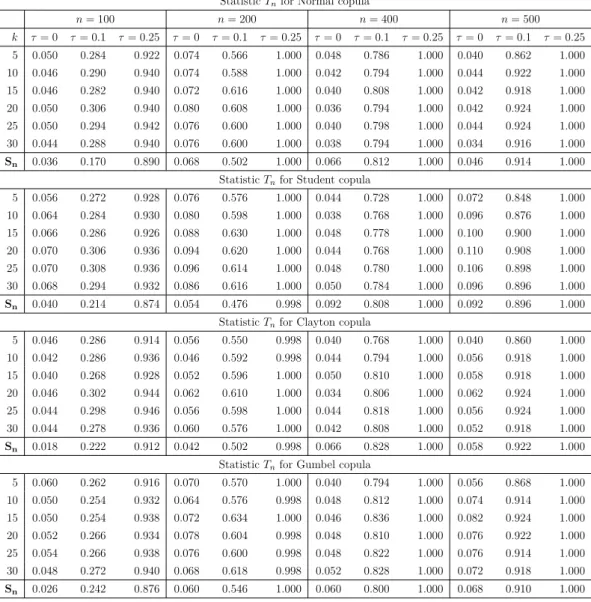
StatisticTnfor Normal copula n= 100 n= 200 n= 400 n= 500 k τ= 0 τ= 0.1 τ= 0.25 τ= 0 τ= 0.1 τ= 0.25 τ= 0 τ= 0.1 τ= 0.25 τ= 0 τ= 0.1 τ= 0.25 5 0.050 0.284 0.922 0.074 0.566 1.000 0.048 0.786 1.000 0.040 0.862 1.000 10 0.046 0.290 0.940 0.074 0.588 1.000 0.042 0.794 1.000 0.044 0.922 1.000 15 0.046 0.282 0.940 0.072 0.616 1.000 0.040 0.808 1.000 0.042 0.918 1.000 20 0.050 0.306 0.940 0.080 0.608 1.000 0.036 0.794 1.000 0.042 0.924 1.000 25 0.050 0.294 0.942 0.076 0.600 1.000 0.040 0.798 1.000 0.044 0.924 1.000 30 0.044 0.288 0.940 0.076 0.600 1.000 0.038 0.794 1.000 0.034 0.916 1.000 Sn 0.036 0.170 0.890 0.068 0.502 1.000 0.066 0.812 1.000 0.046 0.914 1.000 StatisticTnfor Student copula

5 0.056 0.272 0.928 0.076 0.576 1.000 0.044 0.728 1.000 0.072 0.848 1.000 10 0.064 0.284 0.930 0.080 0.598 1.000 0.038 0.768 1.000 0.096 0.876 1.000 15 0.066 0.286 0.926 0.088 0.630 1.000 0.048 0.778 1.000 0.100 0.900 1.000 20 0.070 0.306 0.936 0.094 0.620 1.000 0.044 0.768 1.000 0.110 0.908 1.000 25 0.070 0.308 0.936 0.096 0.614 1.000 0.048 0.780 1.000 0.106 0.898 1.000 30 0.068 0.294 0.932 0.086 0.616 1.000 0.050 0.784 1.000 0.096 0.896 1.000 Sn 0.040 0.214 0.874 0.054 0.476 0.998 0.092 0.808 1.000 0.092 0.896 1.000 StatisticTnfor Clayton copula

5 0.060 0.262 0.916 0.070 0.570 1.000 0.040 0.794 1.000 0.056 0.868 1.000 10 0.050 0.254 0.932 0.064 0.576 0.998 0.048 0.812 1.000 0.074 0.914 1.000 15 0.050 0.254 0.938 0.072 0.634 1.000 0.046 0.836 1.000 0.082 0.924 1.000 20 0.052 0.266 0.934 0.078 0.604 0.998 0.048 0.810 1.000 0.076 0.922 1.000 25 0.054 0.266 0.938 0.076 0.600 0.998 0.048 0.822 1.000 0.076 0.914 1.000 30 0.048 0.272 0.940 0.068 0.618 0.998 0.052 0.828 1.000 0.072 0.918 1.000 Sn 0.026 0.242 0.876 0.060 0.546 1.000 0.060 0.800 1.000 0.068 0.910 1.000

Table 4. This table compares the empirical size and power of the test statistics Tn and Sn for different

cop-ulas (Normal, Student, Clayton and Gumbel copcop-ulas) with estimated marginal distributions, different values of Kendall’s tau coefficientτ(τ= 0,0.1,0.25), different sample sizesn(n= 100,200,400,500), and different values for the bandwidthk.

(21)

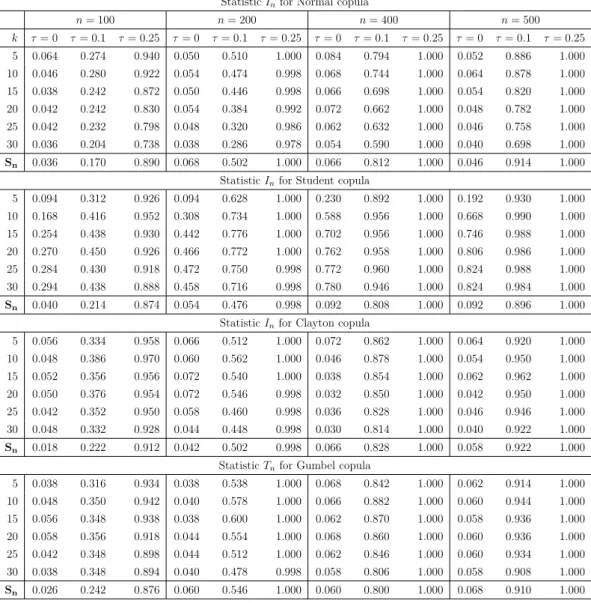
StatisticInfor Normal copula n= 100 n= 200 n= 400 n= 500 k τ= 0 τ= 0.1 τ= 0.25 τ= 0 τ= 0.1 τ= 0.25 τ= 0 τ= 0.1 τ= 0.25 τ= 0 τ= 0.1 τ= 0.25 5 0.064 0.274 0.940 0.050 0.510 1.000 0.084 0.794 1.000 0.052 0.886 1.000 10 0.046 0.280 0.922 0.054 0.474 0.998 0.068 0.744 1.000 0.064 0.878 1.000 15 0.038 0.242 0.872 0.050 0.446 0.998 0.066 0.698 1.000 0.054 0.820 1.000 20 0.042 0.242 0.830 0.054 0.384 0.992 0.072 0.662 1.000 0.048 0.782 1.000 25 0.042 0.232 0.798 0.048 0.320 0.986 0.062 0.632 1.000 0.046 0.758 1.000 30 0.036 0.204 0.738 0.038 0.286 0.978 0.054 0.590 1.000 0.040 0.698 1.000 Sn 0.036 0.170 0.890 0.068 0.502 1.000 0.066 0.812 1.000 0.046 0.914 1.000 StatisticInfor Student copula

5 0.094 0.312 0.926 0.094 0.628 1.000 0.230 0.892 1.000 0.192 0.930 1.000 10 0.168 0.416 0.952 0.308 0.734 1.000 0.588 0.956 1.000 0.668 0.990 1.000 15 0.254 0.438 0.930 0.442 0.776 1.000 0.702 0.956 1.000 0.746 0.988 1.000 20 0.270 0.450 0.926 0.466 0.772 1.000 0.762 0.958 1.000 0.806 0.986 1.000 25 0.284 0.430 0.918 0.472 0.750 0.998 0.772 0.960 1.000 0.824 0.988 1.000 30 0.294 0.438 0.888 0.458 0.716 0.998 0.780 0.946 1.000 0.824 0.984 1.000 Sn 0.040 0.214 0.874 0.054 0.476 0.998 0.092 0.808 1.000 0.092 0.896 1.000 StatisticInfor Clayton copula

5 0.038 0.316 0.934 0.038 0.538 1.000 0.068 0.842 1.000 0.062 0.914 1.000 10 0.048 0.350 0.942 0.040 0.578 1.000 0.066 0.882 1.000 0.060 0.944 1.000 15 0.056 0.348 0.938 0.038 0.600 1.000 0.062 0.870 1.000 0.058 0.936 1.000 20 0.058 0.356 0.918 0.044 0.554 1.000 0.068 0.860 1.000 0.060 0.936 1.000 25 0.042 0.348 0.898 0.044 0.512 1.000 0.062 0.846 1.000 0.060 0.934 1.000 30 0.038 0.348 0.894 0.040 0.478 0.998 0.058 0.806 1.000 0.058 0.908 1.000 Sn 0.026 0.242 0.876 0.060 0.546 1.000 0.060 0.800 1.000 0.068 0.910 1.000

Table 5. This table compares the empirical size and power of the test statisticsInandSnfor different copulas

(Normal, Student, Clayton and Gumbel copulas ) with estimated marginal distributions , different values of Kendall’s tau coefficientτ(τ= 0,0.1,0.25), different sample sizesn(n= 100,200,400,500), and different values for the bandwidthk.

(22)

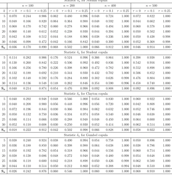
Statisticδnfor Normal copula n= 100 n= 200 n= 400 n= 500 k τ= 0 τ= 0.1 τ= 0.25 τ= 0 τ= 0.1 τ= 0.25 τ= 0 τ= 0.1 τ= 0.25 τ= 0 τ= 0.1 τ= 0.25 5 0.070 0.244 0.906 0.062 0.480 0.996 0.048 0.724 1.000 0.072 0.822 1.000 10 0.048 0.166 0.820 0.064 0.364 0.988 0.048 0.592 1.000 0.044 0.662 1.000 15 0.068 0.170 0.742 0.060 0.278 0.966 0.046 0.494 1.000 0.060 0.578 1.000 20 0.060 0.140 0.612 0.052 0.238 0.930 0.044 0.394 1.000 0.050 0.502 1.000 25 0.042 0.108 0.512 0.044 0.188 0.906 0.038 0.336 1.000 0.050 0.438 0.998 30 0.046 0.098 0.472 0.042 0.166 0.842 0.040 0.300 1.000 0.052 0.368 0.998 Sn 0.036 0.170 0.890 0.068 0.502 1.000 0.066 0.812 1.000 0.046 0.914 1.000 Statisticδnfor Student copula

5 0.114 0.282 0.906 0.176 0.524 0.996 0.366 0.864 1.000 0.398 0.938 1.000 10 0.130 0.260 0.842 0.222 0.506 0.992 0.492 0.836 1.000 0.542 0.916 1.000 15 0.166 0.256 0.780 0.226 0.398 0.960 0.472 0.782 1.000 0.552 0.898 1.000 20 0.132 0.188 0.692 0.210 0.344 0.930 0.432 0.702 1.000 0.506 0.852 1.000 25 0.102 0.148 0.592 0.176 0.284 0.880 0.382 0.626 0.998 0.476 0.804 1.000 30 0.114 0.136 0.548 0.148 0.262 0.846 0.354 0.590 0.996 0.458 0.740 1.000 Sn 0.040 0.214 0.874 0.054 0.476 0.998 0.092 0.808 1.000 0.092 0.896 1.000 Statisticδnfor Clayton copula

5 0.040 0.292 0.948 0.048 0.566 1.000 0.054 0.830 1.000 0.060 0.922 1.000 10 0.040 0.208 0.900 0.056 0.448 0.996 0.056 0.720 1.000 0.042 0.808 1.000 15 0.072 0.196 0.844 0.030 0.366 0.984 0.062 0.632 1.000 0.052 0.746 1.000 20 0.050 0.132 0.750 0.036 0.334 0.974 0.058 0.540 1.000 0.046 0.638 1.000 25 0.046 0.114 0.666 0.030 0.288 0.948 0.048 0.450 1.000 0.064 0.600 1.000 30 0.052 0.110 0.608 0.030 0.250 0.930 0.052 0.414 1.000 0.062 0.514 1.000 Sn 0.018 0.222 0.912 0.042 0.502 0.998 0.066 0.828 1.000 0.058 0.922 1.000 Statisticδnfor Gumbel copula

5 0.038 0.240 0.924 0.038 0.490 0.994 0.054 0.758 1.000 0.050 0.896 1.000 10 0.036 0.188 0.850 0.060 0.398 0.988 0.064 0.638 1.000 0.038 0.786 1.000 15 0.050 0.192 0.782 0.054 0.318 0.966 0.044 0.556 1.000 0.060 0.714 1.000 20 0.038 0.138 0.686 0.048 0.272 0.948 0.048 0.480 0.998 0.054 0.648 1.000 25 0.036 0.118 0.600 0.042 0.218 0.898 0.050 0.426 0.998 0.062 0.580 1.000 30 0.044 0.110 0.514 0.050 0.212 0.860 0.052 0.388 0.994 0.048 0.510 1.000 Sn 0.026 0.242 0.876 0.060 0.546 1.000 0.060 0.800 1.000 0.068 0.910 1.000

Table 6. This table compares the empirical size and power of the test statistics δn and Snfor different

copu-las (Normal, Student, Clayton and Gumbel copucopu-las) with estimated marginal distributions, different values of Kendall’s tau coefficientτ(τ= 0,0.1,0.25), different sample sizesn(n= 100,200,400,500), and different values for the bandwidthk.

(23)

References

Bilodeau, M., and Lafaye de Micheaux, M. (2005), ‘A multivariate empirical characteristic func-tion test of independence with normal marginals’,Journal of Multivariate Analysis, 95, 345– 369.

Blum, J., Kiefer, J., and Rosenblatt, M. (1961), ‘Distribution Free Tests of Independence Based on the Sample Distribution Function’,Annals of Mathematical Statistics, 32, 485–498. Blumentritt, T., and Schmid, F. (2012), ‘Mutual information as a measure of multivariate

associ-ation: analytical properties and statistical estimation’,Journal of Statistical Computation and Simulation, 82, 1257–1274.

Borkowf, C.B. (2002), ‘Computing the nonnull asymptotic variance and the asymptotic relative efficiency of Spearman’s rank correlation’,Computational statistics and data analysis, 39, 271– 286.

Bouezmarni, T., Rombouts, J., and Taamouti, A. (2010), ‘Asymptotic properties of the Bernstein density copula estimator forα-mixing data’,Journal of Multivariate Analysis, 101, 1–10. Deheuvels, P. (1979), ‘La Fonction de Dépendance Empirique et ses Propriétés. Un Test non

Param´etrique D’independance’,Bullettin de l’acad´emie Royal de Belgique, Classe des Sciences, 65, 274–292.

Deheuvels, P. (1981a), ‘An asymptotic decomposition for multivariate distribution-free test of independence’,Journal of Multivariate Analysis, 11, 102 – 113.

Deheuvels, P. (1981b), ‘A Kolmogorov-Smirnov type test for independence and multivariate sam-ples’,Rev. Roumaine Mtah. Pures Appl., 26, 213–226.

Deheuvels, P. (1981c), ‘A nonparametric test of independence’, Pulication de Statistique de l’Universit´e de Paris, 26, 29–50.

Dugué, D. (1975), ‘Sur les tests d’indépendance ‘indépendants de la loi”, Comptes rendus de l’Académie des Sciences de Paris, Série A, 281, 1103–1104.

Feuerverger, A. (1993), ‘A consitent test for bivariate dependence’,International Statistical Re-view, 61, 419–433.

Genest, C., and R´emillard, B. (2004), ‘Test of independence or randomness based on the empirical copula process’,Test, 13, 335–369.

Genest, C., Quessy, J., and R´emillard, B. (2006), ‘Local efficiency of Cram´er-von Mises test of independence’,Journal of Multivariate Analysis, 97, 274–294.

Ghoudi, K., Kulperger, R., and R´emillard, B. (2001), ‘A nonparametric test of serial independence for time series and residuals’,Journal of Multivariate Analysis, 79, 191–218.

Hall, P. (1984), ‘Central Limit Theorem for Integrated Square Error of Multivariate Nonpara-metric Density Estimators’,Journal of Multivariate Analysis, 14, 1–16.

Janssen, P., Swanepoel, J., and Veraverbeke, N. (2012), ‘Large sample behavior of the Bernstein copula estimator’,Journal of Statistical Planing and Inference., 142, 1189–1197.

Janssen, P., Swanepoel, J., and Veraverbeke, N. (2014), ‘A note on the asymptotic bevahior of the Bernstein estimator of the copula density’,Journal of Multivariate Analysis, 124, 480–487. Joe, H. (1989a), ‘Estimation of entropy and other functionals of a multivariate density’,Annals

(24)

Joe, H. (1989b), ‘Relative entropy measures of multivariate dependence’,Journal of the American Statistical Association, 84, 157–164.

Joe, H., et al. (1987), ‘Majorization, randomness and dependence for multivariate distributions’,

The Annals of Probability, 15, 1217–1225.

Kojadinovic, I., and Holmes, M. (2009), ‘Tests of independence among continuos random vectors based on Cram´er-von Mises functionals of the empirical copula process’,Journal of Multivariate Analysis, 100(6), 1137–1154.

Nelsen, R. (2006),An Introduction to Copulas, Springer, New York.

Omelka, M., Gijbels, I., and Veraverbeke, N. (2009), ‘Improved Kernel Estimation of Copulas: Weak Convergence and Goodnees-of-Fit Testing’,Annals of Statistics, 37, 3023–3058.

Prokhorov, A.V. (2001), Kendall Coefficient of Rank Correlation in Hazewinkel, Michiel, Ency-clopedia of Mathematics, Springer.

Rota, G. (1964), ‘On the Foundations of Combinatorial Theory. I. Theory of Mobius Functions’,

Zeitschrift fur Wahrscheinlichkeitstheorie und verwandte Gebiete, 2, 340–368.

Sancetta, A., and Satchell, S. (2004), ‘The Bernstein Copula and its Applications to Modeling and Approximations of Multivariate Distributions’,Econometric Theory, 20, 535–562. Sklar, A. (1959), ‘Fonction de R´epartition `a n Dimensions et leurs Marges’, Publications de

l’Institut de Statistique de l’Universit´e de Paris, 8, 229–231.

Stute, W. (1984), ‘The oscillation behavior of empirical processes: The multivariate case’, The Annals of Probability, pp. 361–379.

(25)

Appendix A. Proofs of Propositions 1, 3, 4, 5, and of Theorem 2

Proof of Proposition 1.First of all, we decompose the test statisticTn in the following

way: Tn=n Z [0,1]d  Ck,n(u)− d Y j=1 uj   2 du1...dud =n Z [0,1]d(Ck,n( u))2du1...dud−2n Z [0,1]dCk,n( u) d Y j=1 ujdu1...dud +n Z [0,1]d   d Y j=1 uj   2 du1...dud =T1n−T2n+T3n. Furthermore, we have T1n =n Z [0,1]d (Ck,n(u))2du1...dud =n Z [0,1]d X (v,s) Cn _v 1 k , ..., vd k Cn _s 1 k, ..., sd k × d Y j=1 Pvj,k(uj)Psj,k(uj)du1...dud.

Using the definition of binomial distribution, we obtain T1n =n X (v,s) k v1 ...kvd k s1 ...ksd Cn _v 1 k , ..., vd k Cn _s 1 k, ..., sd k × Z [0,1]d d Y j=1 uvj+sj₍₁₋_u₎2k−vj−sj_du 1...dud =nX (v,s) Cn _v 1 k, ..., vd k Cn _s 1 k , ..., sd k × d Y j=1 k vj k sj β(vj+sj+ 1,2k−vj−sj+ 1).

In a similar way, we can show that

T2n = 2n k X v1=0 ... k X vd=1 Cn _v 1 k, ..., vd k d Y j=1 _k vj β(vj+ 2, k−vj+ 1).

(26)

Proof of Proposition 3. We provide the proof for d = 2. The generalization to d >2 is straightforward. For a two-dimensional vector u = (u1, u2), we start by the following decomposition: Z ˆ Cn,k(u)−u1u2 2 du= Z ˆ Cn,k(u)−C(u) 2 du+ Z (C(u)−u1u2)2 du + 2 Z ˆ Cn,k(u)−C(u) (C(u)−u1u2) du =T1,n+T2,n+T3,n.

From Janssen et al.(2012) and the continuous mapping theorem we have n Z ˆ Cn,k(u)−C(u) 2 du=Op(1). (A1)

Furthermore, from Janssen et al. (2012) , we can show that n Z ˆ Cn,k(u)−C(u) (C(u)−u1u2) du=op(n). (A2)

Therefore, using the fact that R

(C(u, v)−u1u2)2du > 0 and from (A1) and (A2), we deduce the consistency of Tn.

Proof of Proposition 4. Expanding the squared term in the test statistic (10) leads to the following decomposition:

In =In(1)+I (2) n + 1, with I_n(1)= Z [0,1]2 c2_k,n(u)du and I_n(2)=−2 Z [0,1]2 ck,n(u)du. First, by writing c2k,n(u) =k 4 k−1 X v1,v01=0 v2,v02=0 Υk(v1, v2)Υk(v01, v20)Pv1,k−1(u1)Pv₁0,k−1(u1)Pv2,k−1(u2)Pv₂0,k−1(u2),

(27)

we deduce that In(1)(u) =k4 k−1 X v1,v01=0 v2,v02=0 Υk(v1, v2)Υk(v01, v02) × Z 1 0 Z 1 0 Pv1,k−1(u1)Pv0₁,k−1(u1)Pv2,k−1(u2)Pv₂0,k−1(u2)du1du1 =k4 k−1 X v1,v0₁=0 v2,v0₂=0 Υk(v1, v2)Υk(v01, v 0 2)Γk(v1, v10)Γk(v2, v02).

Second, from the definition of cn,k(.) in Equation (8), we have

Z [0,1]2ck,n(u)du= k X v1,v2=0 Cn _v 1 k, v2 k Z 1 0 Z 1 0 Pv01,k(u1)P 0 v2,k(u2)du1du2. As R [0,1]P 0 v1,k(u) =Pv1,k(u)| 1

0=I{v1= 0}+I{v1=k}, the last integral is equal to 1.

Proof of Theorem 1 ford= 2. The following proof corresponds to the bivariate case. For the more general case d > 2, the proof can be obtained in a similar way. For the bivariate case (d =2), we will show that the random variable

In,k :=nk−2        In−2−2πn−1k 21/2 r n Pk−1 v1,v2=0Γ 2 k(v1, v2) o2 −k−4        (A3)

is asymptotically normally distributed. First, observe that dealing with term In in (A3)

is quite tricky since it involves the pseudo-observations V1, . . . ,Vn. Thus, we consider

e In= R [0,1]2{_eck,n(u)−1}2du, where forVie = (F₁(X_i,₁), F₂(X_i,₂)), e ck,n(u) := k X v1,v2=0 e Cn _v 1 k , v2 k Pv01,k(u1)P 0 v2,k(u2) and Cen(u) =n −1 n X i=1 I{Vie ≤u}.

The new term Ie_n is just a version ofI_n in which the pseudo-observationsV₁, . . . ,Vn have

been replaced with “uniformized” observations Ve₁, . . . ,Vne . Under the null hypothesis,

e

Vi = (Vei,1,Vei,2) are independent and uniformly distributed random variables.

We now define a new term Ie_n,k which is equal to the term in the right hand side of

Equation (A3) after replacing In by Ie_n. In the following, the proof of Theorem 1 will

be obtained in two steps. In a first step, we show that Ie_n,k is asymptotically normally

(28)

A.1. Asymptotic normality of In,ke

Using the decomposition in the proof of Proposition 4, we can obtain the following de-composition: e In =Ie₁_n+Ie₂_n−1, where e I1n = k4n−2 n X i=1 k−1 X v,v0₌₀ I{Vie ∈A_k(v₁, v₂)}Γ_k(v₁, v₁)Γ_k(v₂, v₂) e I2n = 2k4n−2 n X i<j Pn(Vie ,Vje ), with Pn(Vie ,Vje ) =Pk_v−_,_v10₌₀_I{Vie ∈A_k(v₁, v₂)}_I{Ve_j ∈A_k(v₁0, v₂0)}Γ_k(v₁, v₁0)Γ_k(v₂, v₂0).

We start by studying the first term Ie₁_n. As E I{Vie ∈A_k(v₁, v₂)} =k−2_{, we get} EIe₁_n =k2n−1 (k−1 X v1=0 Γ2_k(v1, v1) ) .

Next, using Lemma 2 in Janssen et al. (2014), we have

k−1 X v1=0 Pv21,k−1(u) = k−1/2 p 4πu(1−u) +o(k −1/2₎ . Then, EIe₁_n = π 4kn −1₊_o₍_kn−1₎_.

Thereafter, as Var( I{Vie ∈A_k(v₁, v₂)}) =k−2−k−4, we deduce that

VarIe₁_n =k8n−3(k−2−k−4) (_k₋₁ X v1=0 Γ2_k(v1, v1) )2 .

Then, from Lemma5, we can conclude that

e I1n = E e I1n +nIe₁_n−E e I1n o = π 4kn −1₊_O P(n−3/2k3/2).