ESTIMATION OF REMAINING SERVICE LIFE OF FLEXIBLE PAVEMENTS FROM SURFACE DEFLECTIONS
by
DABA SHABARA GEDAFA
B.S., Addis Ababa University, Ethiopia, 2001
M.Tech., Indian Institute of Technology Bombay, India, 2005
AN ABSTRACT OF A DISSERTATION
submitted in partial fulfillment of the requirements for the degree DOCTOR OF PHILOSOPHY
Department of Civil Engineering College of Engineering
KANSAS STATE UNIVERSITY Manhattan, Kansas
Abstract
Remaining service life (RSL) has been defined as the anticipated number of years that a pavement will be functionally and structurally acceptable with only routine maintenance. The Kansas Department of Transportation (KDOT) has a comprehensive pavement management system, network optimization system (NOS), which uses the RSL concept. In support of NOS, annual condition surveys are conducted on the state highway system. Currently KDOT uses an empirical equation to compute RSL of flexible pavements based on surface condition and deflection from the last sensor of a falling-weight deflectometer (FWD). Due to limited resources and large size, annual network-level structural data collection at the same rate as the project level is impractical. A rolling-wheel deflectometer (RWD), which measures surface deflections at highway speed, is an alternate and fast method of pavement-deflection testing for network-level data collection. Thus, a model that can calculate RSL in terms of FWD first sensor/center deflection (the only deflection measured by RWD) is desired for NOS.
In this study, RWD deflection data was collected under an 18-kip axle load at highway speed on non-Interstate highways in northeast Kansas in July 2006. FWD deflection data,
collected with a Dynatest 8000 FWD on the KDOT network from 1998 to 2006, were reduced to mile-long data to match the condition survey data collected annually for NOS. Normalized and temperature-corrected FWD and RWD center deflections and corresponding effective structural numbers (SNeff) were compared. A nonlinear regression procedure in Statistical Analysis Software (SAS) and Solver in Microsoft Excel were used to develop the models in this study.
Results showed that FWD and RWD center deflections and corresponding SNeff are statistically similar. Temperature-correction factors have significant influence on these variables. FWD data analysis on the study sections showed that average structural condition of pavements of the KDOT non-Interstate network did not change significantly over the last four years. Thus, network-level deflection data can be collected at four-year intervals when there is no major structural improvement.
Results also showed that sigmoimal relationship exists between RSL and center
deflection. Sigmoidal RSL models have very good fits and can be used to predict RSL based on center deflection from FWD or RWD. Sigmoidal equivalent fatigue crack-models have also
shown good fits, but with some scatter that can be attributed to the nature and quality of the data used to develop these models. Predicted and observed equivalent transverse-crack values do not match very well, though the difference in magnitude is insignificant for all practical purposes.
ESTIMATION OF REMAINING SERVICE LIFE OF FLEXIBLE PAVEMENTS FROM SURFACE DEFLECTIONS
by
DABA SHABARA GEDAFA
B.S., Addis Ababa University, Ethiopia, 2001
M.Tech., Indian Institute of Technology Bombay, India, 2005
A DISSERTATION
submitted in partial fulfillment of the requirements for the degree DOCTOR OF PHILOSOPHY
Department of Civil Engineering College of Engineering
KANSAS STATE UNIVERSITY Manhattan, Kansas
2008
Approved by: Major Professor Dr. Mustaque Hossain
Copyright
DABA SHABARA GEDAFA 2008
Abstract
Remaining service life (RSL) has been defined as the anticipated number of years that a pavement will be functionally and structurally acceptable with only routine maintenance. The Kansas Department of Transportation (KDOT) has a comprehensive pavement management system, network optimization system (NOS), which uses the RSL concept. In support of NOS, annual condition surveys are conducted on the state highway system. Currently KDOT uses an empirical equation to compute RSL of flexible pavements based on surface condition and deflection from the last sensor of a falling-weight deflectometer (FWD). Due to limited resources and large size, annual network-level structural data collection at the same rate as the project level is impractical. A rolling-wheel deflectometer (RWD), which measures surface deflections at highway speed, is an alternate and fast method of pavement-deflection testing for network-level data collection. Thus, a model that can calculate RSL in terms of FWD first sensor/center deflection (the only deflection measured by RWD) is desired for NOS.
In this study, RWD deflection data was collected under an 18-kip axle load at highway speed on non-Interstate highways in northeast Kansas in July 2006. FWD deflection data,
collected with a Dynatest 8000 FWD on the KDOT network from 1998 to 2006, were reduced to mile-long data to match the condition survey data collected annually for NOS. Normalized and temperature-corrected FWD and RWD center deflections and corresponding effective structural numbers (SNeff) were compared. A nonlinear regression procedure in Statistical Analysis Software (SAS) and Solver in Microsoft Excel were used to develop the models in this study.
Results showed that FWD and RWD center deflections and corresponding SNeff are statistically similar. Temperature-correction factors have significant influence on these variables. FWD data analysis on the study sections showed that average structural condition of pavements of the KDOT non-Interstate network did not change significantly over the last four years. Thus, network-level deflection data can be collected at four-year intervals when there is no major structural improvement.
Results also showed that sigmoimal relationship exists between RSL and center
deflection. Sigmoidal RSL models have very good fits and can be used to predict RSL based on center deflection from FWD or RWD. Sigmoidal equivalent fatigue crack-models have also
shown good fits, but with some scatter that can be attributed to the nature and quality of the data used to develop these models. Predicted and observed equivalent transverse-crack values do not match very well, though the difference in magnitude is insignificant for all practical purposes.
Table of Contents
List of Figures ... xvii
List of Tables ... xxiii
Acknowledgements ... xxvii
Dedication ... xxviii
CHAPTER 1 INTRODUCTION ... 1
1.1 General ... 1
1.2 Problem Statement ... 3
1.3 Objectives of the Study ... 5
1.4 Organization of Dissertation ... 5
CHAPTER 2 LITERATURE REVIEW ... 6
2.1 Introduction ... 6
2.2 Pavement Management System ... 6
2.2.1 Basic Components ... 7
2.2.2 Pavement Management Levels ... 7
2.3 Kansas Department of Transportation (KDOT) PMS ... 8
2.3.1 Methodology for KDOT Network Optimization System (NOS) ... 9
2.3.2 Implementation of the NOS ... 10
2.3.2.1 Identification of Road Categories ... 10
2.3.2.2 Determination of Distress Types, Influence Variables, and Distress States ... 10
2.3.2.3 Condition States (CS) ... 10
2.3.2.4 Feasible Maintenance and Rehabilitation Actions ... 12
2.3.2.5 Costs of Different Actions ... 12
2.3.2.6 Optimal Rehabilitation Policies ... 13
2.3.3 Project Optimization System (POS) ... 14
2.3.4 Pavement Management Information System (PMIS) ... 14
2.4 Remaining Service Life (RSL) ... 14
2.4.1 RSL Estimation Procedures ... 15
2.4.1.2 Structural Failure-Based Approaches ... 19
2.4.1.3 Functional and Structural Failure-Based Approaches ... 21
2.5 Pavement Performance Prediction ... 21
2.5.1 Classification of Performance Prediction Models ... 23
2.6 Model Development ... 25
2.6.1 Nonlinear Regression Procedure in Statistical Analysis Software (SAS) ... 26
2.6.1.1 Computational Methods ... 27
2.6.1.1.1 Gauss-Newton ... 28
2.6.1.1.2 Newton ... 28
2.6.1.1.3 Marquardt ... 29
2.6.1.1.4 Gradient... 29
2.7 Pavement Deflection Devices ... 29
2.7.1 Static or Slow-Moving Devices ... 30
2.7.2 Steady State Devices ... 30
2.7.3 Impact (Impulse)-Load Response Devices ... 33
2.7.3.1 Falling-Wheel Deflectometer (FWD) ... 33
2.7.4 Automated Mobile Dynamic-Load-Method Devices ... 35
2.7.4.1 Rolling-Wheel Deflectometer (RWD) ... 35
2.7.4.1.1 Deflection Measurement Principle ... 38
2.7.4.1.2 Data Acquisition System, Operating and Data Analysis Software . 38 2.8 Correcting Deflections for Pavement Temperature ... 39
2.8.1 Pavement Temperature Prediction ... 39
2.8.2 Deflection Correction ... 42
2.9 Pavement Structural Capacity ... 44
2.10 Integration of Pavement Deflection Data into PMS ... 48
2.11 Summary of Literature Review ... 49
CHAPTER 3 TEST SECTIONS AND DATA COLLECTION ... 50
3.1 Test Sections ... 50
3.1.1 Experimental Sections ... 50
3.1.2 Highway Network ... 52
3.2.1 RWD Deflection Data ... 54
3.2.2 FWD Deflection Data ... 54
3.3 Stress-and-Strain Data ... 54
3.4 Temperature Data... 55
3.4.1 Pavement Surface Temperature ... 55
3.4.2 Pavement Mid-Depth Temperature ... 56
3.5 KDOT PMS Data ... 56
3.5.1 Cracking Data ... 56
3.5.1.1 Fatigue Cracking Data ... 56
3.5.1.2 Transverse Cracking Data ... 57
3.5.2 Rutting Data ... 58
3.5.3 Layer Thickness ... 59
3.5.4 Traffic Data ... 59
3.5.5 RSL Data ... 60
CHAPTER 4 DATA ANALYSIS AND DISCUSSIONS ... 61
4.1 Introduction ... 61 4.2 Deflection Data ... 61 4.2.1 Repeatability ... 62 4.2.1.1 Repeatability of RWD ... 62 4.2.1.2 Repeatability of FWD ... 62 4.2.1.3 Significant-Difference Test ... 63
4.2.2 FWD and RWD Center Deflection ... 64
4.2.2.1 Experimental Sections ... 65
4.2.2.2 Without Rehabilitation Actions ... 66
4.2.2.3 With Rehabilitation Actions ... 67
4.2.2.4 Significant-Difference Test ... 68
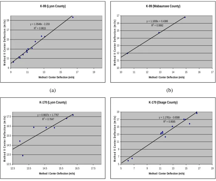
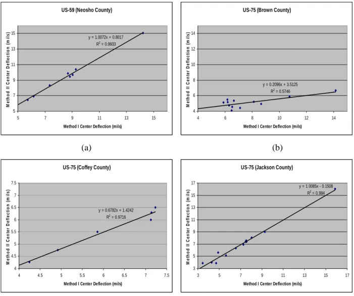
4.2.2.5 Linear Regression ... 72
4.2.3 Effect of Temperature-Correction Method ... 74
4.2.3.1 Kansas Routes ... 75
4.2.3.2 US Routes ... 77
4.2.3.4 Linear Regression ... 80
4.2.4 Frequency of Deflection Measurement Using FWD Center Deflection ... 82
4.2.4.1 Without Rehabilitation Actions ... 82
4.2.4.2 With Rehabilitation Actions ... 84
4.2.4.3 Significant-Difference Test ... 85
4.2.4.4 Linear Regression ... 87
4.2.5 Measured and Calculated Pavement Temperature ... 88
4.2.5.1 Spring 2006 ... 88
4.2.5.2 Summer 2006 ... 90
4.2.5.3 Fall 2006 ... 91
4.2.5.4 Significant-Difference Test ... 92
4.3 Pavement Structural Capacity ... 94
4.3.1 FWD and RWD SNeff ... 94
4.3.1.1 Experimental Sections ... 95
4.3.1.2 Without Rehabilitation Actions ... 96
4.3.1.3 With Rehabilitation Actions ... 97
4.3.1.4 Significant-Difference Test ... 99
4.3.1.5 Linear Regression ... 102
4.3.2 Effect of Temperature-Correction Method on SNeff ... 102
4.3.2.1 Kansas Routes ... 104
4.3.2.2 US Routes ... 106
4.3.2.3 Significant-Difference Test ... 108
4.3.2.4 Linear Regression ... 109
4.3.3 Frequency of Deflection Measurements Using SNeff ... 111
4.3.3.1 Without Rehabilitation Actions ... 111
4.3.3.2 With Rehabilitation Actions ... 113
4.3.3.3 Significant-Difference Test ... 114
4.3.4 AASHTO and KDOT SNeff ... 115
4.3.4.1 Experimental Sections ... 117
4.3.4.2 Road Category-Wise ... 118
4.3.4.4 Significant-Difference Test ... 122
CHAPTER 5 PREDICTION MODELS ... 124
5.1 Introduction ... 124
5.2 Model Development ... 124
5.2.1 NLIN Procedure ... 126
5.2.2 Solver Procedure ... 126
5.2.3 Goodness of Fit ... 127
5.2.4 Mean Absolute Deviation ... 127
5.3 Remaining Service Life (RSL) Models ... 127
5.3.1 Linear Regression ... 128
5.3.1.1 Experimental Sections ... 128
5.3.1.2 Road Category (RC)-Wise ... 129
5.3.1.3 District-Wise and Statewide ... 129
5.3.1.4 Summary of RSL Linear Regression ... 131
5.3.2 RSL Sigmoidal Model with Linear Sub-Models ... 131
5.3.2.1 Road Category (RC)-Wise ... 131
5.3.2.1.1 Model Plots ... 134
5.3.2.1.2 Validation Plots ... 137
5.3.2.2 District-Wise and Statewide ... 139
5.3.2.2.1 Model Plots ... 141
5.3.2.2.2 Validation Plots ... 143
5.3.2.3 Mean Absolute Deviation ... 144
5.3.3 Sigmoidal RSL Model with Quadratic Sub-Models ... 145
5.3.3.1.1 Model Plots ... 149
5.3.3.1.2 Validation Plots ... 151
5.3.3.2 Mean Absolute Deviation ... 153
5.3.4 Sigmoidal RSL Model Using Statewide Data ... 153
5.3.4.1 Model Plots ... 155
5.3.4.2 Validation Plots ... 155
5.3.4.3 Mean Absolute Deviation ... 156
5.3.5.1 Road Category-Wise ... 157
5.3.5.2 District-Wise and Statewide ... 160
5.4 Fatigue Cracking Models ... 161
5.4.1 Linear Regression ... 162
5.4.1.1 Road Category-Wise ... 162
5.4.1.2 District-Wise and Statewide ... 163
5.4.1.3 Summary of Linear EFCR Regression ... 163
5.4.2 Quadratic Regression ... 163
5.4.3 Sigmoidal EFCR Model with Linear Sub-Models ... 164
5.4.3.1 Road Category-Wise ... 164
5.4.3.1.1 Model Plots ... 167
5.4.3.1.2 Validation Plots ... 170
5.4.3.2 District-Wise and Statewide ... 172
5.4.3.2.1 Model Plots ... 174
5.4.3.2.2 Validation Plots ... 176
5.4.3.3 Mean Absolute Deviation ... 177
5.4.4 Sigmoidal EFCR Model with Quadratic Sub-Models ... 179
5.4.4.1.1 Model Plots ... 183
5.4.4.1.2 Validation Plots ... 185
5.4.4.2 Mean Absolute Deviation ... 187
5.4.5 Sigmoidal EFCR Model Using Statewide Data ... 187
5.4.5.1 Model Plots ... 189
5.4.5.2 Validation Plots ... 189
5.4.5.3 Mean Absolute Deviation ... 190
5.5 ETCR Models ... 190
5.5.1 Linear Regression ... 190
5.5.1.1 Road Category-Wise ... 190
5.5.1.2 District-Wise and Statewide ... 190
5.5.1.3 Summary of Linear ETCR Models ... 191
5.5.2 Quadratic Regression ... 191
5.5.3.1 Road Category-Wise ... 193
5.5.3.1.1 Model Plots ... 195
5.5.3.1.2 Validation Plots ... 198
5.5.3.2 District-Wise and Statewide ... 200
5.5.3.2.1 Model Plots ... 202
5.5.3.2.2 Validation Plots ... 204
5.5.3.3 Absolute Mean Deviation ... 205
5.5.4 Sigmoidal ETCR Model with Quadratic Sub-Models ... 207
5.5.4.1.1 Model Plots ... 211
5.5.4.1.2 Validation Plots ... 213
5.5.4.2 Mean Absolute Deviation ... 214
5.5.5 Sigmoidal ETCR Model Using Statewide Data ... 215
5.5.5.1 Model Plots ... 217
5.5.5.2 Validation Plots ... 218
5.5.5.3 Absolute Mean Deviation ... 219
CHAPTER 6 CONCLUSIONS AND RECOMMENDATIONS ... 220
6.1 Conclusions ... 220
6.2 Recommendations ... 222
References ... 223
Appendix A - Data Analysis ... 238
Deflection Data ... 238
FWD and RWD Center Deflection ... 238
Without Rehabilitation Actions ... 238
With Rehabilitation Actions ... 239
Effect of Temperature-Correction Method on Center Deflection ... 241
Route and County-Wise ... 241
Route-Wise ... 242
County-Wise ... 243
District-Wise ... 245
Significant-Difference Test ... 245
Frequency of Deflection Measurement Using Center Deflection ... 248
Without Rehabiltation Actions ... 248
With Rehabilitation Actions ... 248
Measured and Calculated Pavement Temperature ... 249
Pavement Structural Capacity ... 253
FWD and RWD SNeff ... 253
Without Rehabilitation Actions ... 253
With Rehabilitation Actions ... 254
Effect of Temperature-Correction Method on SNeff ... 255
County and Route-Wise ... 255
Route-Wise ... 256
County-Wise ... 258
District-Wise ... 259
Significant-Difference Test ... 259
Linear Regression ... 261
Frequency of Deflection Measurement Using SNeff ... 262
With Rehabilitation Actions ... 262
Without Rehabilitation Actions ... 262
Linear Regression ... 263
SNeff AASHTO and KDOT ... 264
District-Wise and Statewide ... 264
Linear Regression ... 265
Appendix B - Prediction Models ... 266
Strain ... 266 Longitudinal Strain ... 266 Transverse Strain ... 270 Stress on Subgrade ... 274 Significant-Difference Test ... 278 Strain ... 278 Longitudinal Strain ... 278 Transverse Strain ... 279
Stress on Subgrade ... 280 Linear Regression ... 281 Strain ... 281 Longitudinal Strain ... 281 Transverse Strain ... 284 RSL Models ... 287 Quadratic Regression ... 287
Sigmoidal RSL Model with Linear Sub-Models without Cracking Data ... 288
Road Category-Wise ... 288
District-Wise and Statewide ... 296
Absolute Mean Deviation ... 301
ETCR Models ... 302
Sigmoidal ETCR Models with Linear Sub-Models without SNeff ... 302
Road Category-Wise ... 302
District-Wise and Statewide ... 310
List of Figures
Figure 2-1 Basic Components of PMS (USDOT, 1991) ... 7
Figure 2-2 PMS Structure and Information Flows (Amekudzi and Attoh-Okine, 1996) ... 8
Figure 2-3 KDOT PMS System (Kulkarni et al., 1988) ... 9
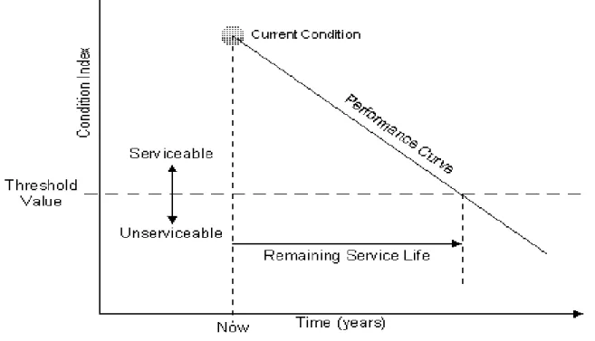
Figure 2-4 Calculating RSL for an Individual Condition Index (FHWA, 1998) ... 16
Figure 2-5 RSL Using Survivor Curve (Vepa et al., 1996) ... 19
Figure 2-6 Relationship between Condition Factor and RSL (AASHTO, 1993) ... 20
Figure 2-7 Pavement Deterioration Curve (FHWA, 1985) ... 22
Figure 2-8 Overview of RWD and Laser D between Dual-Tires (ARA, 2007) ... 37
Figure 2-9 RWD Wheel Configurations and Loads (ARA, 2007) ... 37
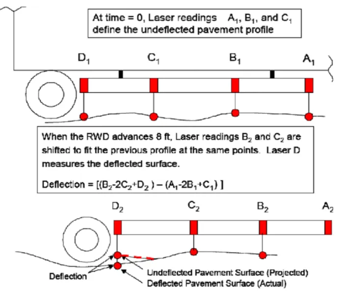
Figure 2-10 Spatially Coincident Profiles of Pavement (Steele et al., undated) ... 39
Figure 3-1 Kansas RWD Test Roads (ARA, 2007) ... 51
Figure 3-2 KDOT FWD Dynatest 8000 ... 55
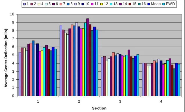
Figure 4-1 Mean FWD and RWD Center Deflections for Experimental Sections ... 63
Figure 4-2 FWD and RWD Center Deflections for Experimental Sections ... 65
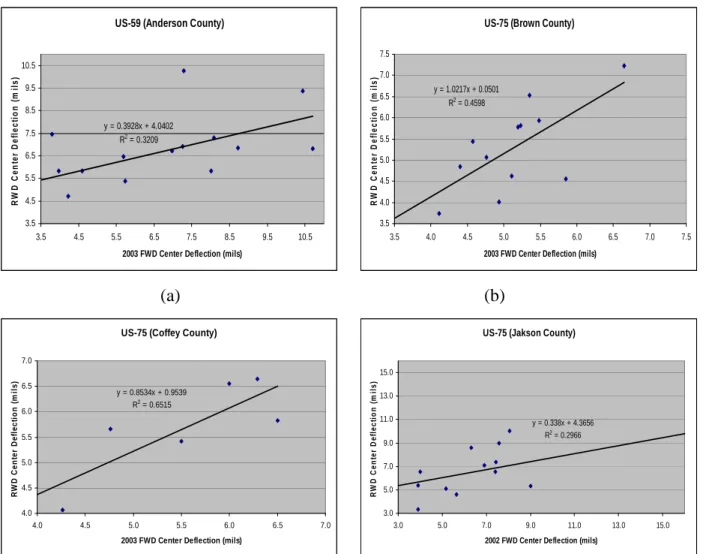
Figure 4-3 FWD and RWD Center Deflections for US-59 and US-75 ... 66
Figure 4-4 FWD and RWD Center Deflections for K-31 and K-99 ... 67
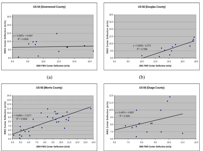
Figure 4-5 FWD and RWD Center Deflections for US-54 and US-56 ... 68
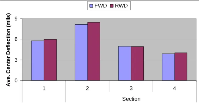
Figure 4-6 Average FWD and RWD Center Deflections for Experimental Sections ... 69
Figure 4-7 Average FWD and RWD Center Deflection ... 70
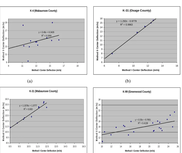
Figure 4-8 Effect of Temperature-Correction Method on FWDd0 for K-4, K-31, and K-99 ... 75
Figure 4-9 Effect of Temperature-Correction Method on FWDd0 for K-99 and K-170 ... 76
Figure 4-10 Effect of Temperature-Correction Method on FWDd0 for US-54 and US-56 ... 77
Figure 4-11 Effect of Temperature-Correction Method on FWDd0 for US-59 and US-75 ... 78
Figure 4-12 Effect of Temperature-Correction Method on Average FWDd0 ... 79
Figure 4-13 FWD Center Deflections over Years for US-54 and US-59 ... 82
Figure 4-14 FWD Center Deflections over Years for US-59 and US-75 ... 83
Figure 4-16 FWD Center Deflection over Years for US-56 ... 85
Figure 4-17 Average FWD Center Deflection over Years ... 86
Figure 4-18 Pavement Temperature for Experimental Sections (Test Date: 04/13/2006) ... 89
Figure 4-19 Pavement Temperature for Experimental Sections (Test Date: 8/1/2006) ... 90
Figure 4-20 Pavement Temperature for Experimental Sections (Test Date: 10/13/2006) ... 91
Figure 4-21 Average Calculated and Measured Mid-Depth Pavement Temperatures ... 92
Figure 4-22 FWD and RWD SNeff for Experimental Sections ... 95
Figure 4-23 FWD and RWD SNeff for US-59 and US-75 ... 96
Figure 4-24 FWD and RWD SNeff for K-31 and K-99 ... 97
Figure 4-25 FWD and RWD SNeff for US-54 and US-56 ... 98
Figure 4-26 FWD and RWD SNeff for Experimental Sections ... 99
Figure 4-27 Average FWD and RWD SNeff ... 100
Figure 4-28 Effect of Temperature-Correction Methods on SNeff for K-4, K-31, and K-99 .... 104
Figure 4-29 Effect of Temperature-Correction Method on SNeff for K-99 and K-170 ... 105
Figure 4-30 Effect of Temperature-Correction Method on SNeff for US-54 and US-56 ... 106
Figure 4-31 Effect of Temperature-Correction Method on SNeff for US-59 and US-75 ... 107
Figure 4-32 Effect of Temperature-Correction Method on Average SNeff ... 108
Figure 4-33 FWD SNeff over Years for US-54 and US-59 ... 111
Figure 4-34 FWD SNeff Over Years for US-59 and US-75 ... 112
Figure 4-35 FWD SNeff over Years for K-31, K-99, and K-170 ... 113
Figure 4-36 FWD SNeff over Years for US-56 ... 114
Figure 4-37 Average FWD SNeff over Years ... 115
Figure 4-38 SNeff AASHTO and KDOT for Experimental Sections ... 117
Figure 4-39 SNeff AASHTO and KDOT for Road Categories 12 to 15 ... 118
Figure 4-40 SNeff AASHTO and KDOT for Road Categories 16 to 19 ... 119
Figure 4-41 SNeff AASHTO and KDOT for Road Categories from 20 to 23 ... 120
Figure 4-42 SNeff AASHTO and KDOT for Districts 1 to 4 ... 121
Figure 4-43 Average SNeff AASHTO and KDOT ... 122
Figure 5-1 Sigmoidal RSL Model with Linear Sub-Models for RC 12 to 15 ... 134
Figure 5-2 Sigmoidal RSL Model with Linear Sub-Models for RC 16 to 19 ... 135
Figure 5-4 Sigmoidal RSL Model with Linear Sub-Models Validation for RC 12 to 15 ... 137
Figure 5-5 Sigmoidal RSL Model with Linear Sub-Models Validation for RC 16 to 19 ... 138
Figure 5-6 Sigmoidal RSL Mode with Linear Sub-Models Validation for RC 20 to 23 ... 139
Figure 5-7 Sigmoidal RSL Model with Linear Sub-Models for Districts 1 to 4 ... 141
Figure 5-8 Sigmoidal RSL Model with Linear Sub-Models for Districts 5, 6, and State ... 142
Figure 5-9 Sigmoidal RSL Models with Linear Sub-Models Validation for Districts 1 to 4 ... 143
Figure 5-10 Sigmoidal RSL Model with Linear Sub-Models Valid. for Dist. 5, 6, and State ... 144
Figure 5-11 Sigmoidal RSL Model with Quadratic Sub-Models for Districts 1 to 4 ... 149
Figure 5-12 Sigmoidal RSL Model with Quadratic Sub-Models for Districts 5, 6, and State ... 150
Figure 5-13 Sigmoidal RSL Model with Quadratic Sub-Models Valid. for Districts 1 to 4 ... 151
Figure 5-14 Sigmoidal RSL Model with Quad. Sub-Models Valid. for Dist. 5, 6, and State .... 152
Figure 5-15 Sigmoidal RSL Model Using Statewide Data ... 155
Figure 5-16 Sigmoidal RSL Model Validation Using Statewide Data ... 156
Figure 5-17 Relationship between RSL and Center Deflection for Road Categories 12 to 15 .. 157
Figure 5-18 Relationship between RSL and Center Deflection for Road Categories 16 to 19 .. 158
Figure 5-19 Relationship between RSL and Center Deflection for Road Categories 20 to 23 .. 159
Figure 5-20 Relationship between RSL and Center Deflection for Districts 1 to 4 ... 160
Figure 5-21 Relationship between RSL and Center Deflection for Districts 5, 6, and State ... 161
Figure 5-22 Sigmoidal EFCR Model with Linear Sub-Models for RC 12 to 15 ... 167
Figure 5-23 Sigmoidal EFCR Model with Linear Sub-Models for RC 16 to 19 ... 168
Figure 5-24 Sigmoidal EFCR Model with Linear Sub-Models for RC 20 to 23 ... 169
Figure 5-25 Sigmoidal EFCR Model with Linear Sub-Models Validation for RC 12 to 15 ... 170
Figure 5-26 Sigmoidal EFCR Model with Linear Sub-Models Validation for RC 16 to 19 ... 171
Figure 5-27 Sigmoidal EFCR Model with Linear Sub-Models Validation for RC 20 to 23 ... 172
Figure 5-28 Sigmoidal EFCR Model with Linear Sub-Models for Districts 1 to 4 ... 174
Figure 5-29 Sigmoidal EFCR Model with Linear Sub-Models for Districts 5, 6, and State ... 175
Figure 5-30 Sigmoidal EFCR Model with Linear Sub-Models Validation for Districts 1 to 4 .. 176
Figure 5-31 Sigmoidal EFCR Model with Linear Sub-models Valid. for Dist. 5, 6, and State . 177 Figure 5-32 Sigmoidal EFCR Model with Quadratic Sub-Models for Districts 1 to 4 ... 183
Figure 5-33 Sigmoidal EFCR Model with Quadratic Sub-Models for Dist. 5, 6, and State ... 184
Figure 5-35 Sigmoidal EFCR Model with Quad. Sub-Models Valid. for Dist. 5, 6, and State.. 186
Figure 5-36 Sigmoidal EFCR Model Using Statewide Data ... 189
Figure 5-37 Sigmoidal EFCR Model Validation Using Statewide Data ... 189
Figure 5-38 Sidmoidal ETCR Model with Linear Sub-Models for RC 12 to 15 ... 195
Figure 5-39 Sidmoidal ETCR Model with Linear Sub-Models for RC 16 to 19 ... 196
Figure 5-40 Sidmoidal ETCR Model with Linear Sub-Models for RC 20 to 23 ... 197
Figure 5-41 Sidmoidal ETCR Model with Linear Sub-Models Validation for RC 12 to 15 ... 198
Figure 5-42 Sidmoidal ETCR Model with Linear Sub-Models Validation for RC 16 to 19 ... 199
Figure 5-43 Sidmoidal ETCR Model with Linear Sub-Models Validation for RC 20 to 23 ... 200
Figure 5-44 Sidmoidal ETCR Model with Linear Sub-Models for Districts 1 to 4 ... 202
Figure 5-45 Sidmoidal ETCR Model with Linear Sub-Models for Districts 5, 6, and State ... 203
Figure 5-46 Sigmoidal ETCR Models with Linear Sub-Models Valid. for Districts 1 to 4 ... 204
Figure 5-47 Sidmoidal ETCR Model with Linear Sub-Models Valid. for Dist. 5, 6, and State . 205 Figure 5-48 Sigmoidal ETCR Model with Quadratic Sub-Models for Districts 1 to 4 ... 211
Figure 5-49 Sigmoidal ETCR Model with Quadratic Sub-Models for Dist. 5, 6, and State ... 212
Figure 5-50 Sigmoidal ETCR Model with Quadratic Sub-Models Valid. for Districts 1 to 4 ... 213
Figure 5-51 Sigmoidal ETCR Model with Quad. Sub-Models Valid. for Dist. 5, 6, and State . 214 Figure 5-52 Sigmoidal ETCR Model Using Statewide Data ... 217
Figure 5-53 Sigmoidal ETCR Model Validation Using Statewide Data ... 218
Figure A-1 FWD and RWD Center Deflections for K-4, US-54, and US-59 ... 238
Figure A-2 FWD and RWD Center Deflections for K-39, K-99, and K-170 ... 239
Figure A-3 FWD and RWD Center Deflections for US-59 and US-75 ... 240
Figure A-4 Effect of Temperature-Correction on FWDd0 for US-59 and US-75 ... 241
Figure A-5 Effect of Temperature-Correction on FWDd0 for K-31, K-99, and K-170 ... 242
Figure A-6 Effect of Temp.-Correction on FWDd0 for US-54, US-56, US-59, and US-75 ... 243
Figure A-7 Effect of Temperature-Correction on Routes in Greenwood and Lyon Counties .... 243
Figure A-8 Effect on Routes in Neosho, Osage, Woodson, and Wabaunsee Counties ... 244
Figure A-9 Effect of Temperature-Correction Method on Routes in Districts 1, 2, and 4 ... 245
Figure A-10 Effect of Temperature-Correction Method on Average FWDd0 ... 245
Figure A-11 FWD Center Deflection over Years for K-4 ... 248
Figure A-13 Comparison of AC-Layer Temperature (Test Date: 09/25/2005) ... 249
Figure A-14 Comparison of AC-Layer Temperature (Test Date: 04/26/2007) ... 251
Figure A-15 FWD and RWD SNeff for K-4, US-54, and US-59 ... 253
Figure A-16 FWD and RWD SNeff for US-59 and US-75 ... 254
Figure A-17 FWD and RWD SNeff for K-39 and K-99 ... 254
Figure A-18 Effect of Temperature-Correction Method on SNeff for US-59 and US-75 ... 255
Figure A-19 Effect of Temperature-Correction Method on SNeff for K-31, K-99, and K-170 . 256 Figure A-20 Effect of Temp.-Correction Method on SNeff US-54, US-56, US-59, and US-75 257 Figure A-21 Effect on Green., Lyon, Neosho, Osage, Wabaunsee, and Woodson Counties ... 258
Figure A-22 Effect of Temperature-Correction Method on SNeff in Districts 1, 2, and 4 ... 259
Figure A-23 Effect of Temperature-Correction Method on Average SNeff ... 259
Figure A-24 FWD SNeff over Years for US-75 ... 262
Figure A-25 FWD SNeff over Years for K-4 ... 262
Figure A-26 SNeff AASHTO and KDOT for Districts 5, 6, and State ... 264
Figure B-1 Average Longitudinal Strain and Center Deflection ... 266
Figure B-2 Maximum Longitudinal Strain and Center Deflection ... 267
Figure B-3 Minimum Longitudinal Strain and Center Deflection ... 268
Figure B-4 Overall Longitudinal Strain and Center Deflection ... 269
Figure B-5 Average Transverse Strain and Center Deflection ... 270
Figure B-6 Maximum Transverse Strain and Center Deflection ... 271
Figure B-7 Minimum Transverse Strain and Center Deflection ... 272
Figure B-8 Overall Transverse Strain and Center Deflection ... 273
Figure B-9 Average Stress on Subgrade and Center Deflection ... 274
Figure B-10 Maximum Stress on Subgrade and Center Deflection ... 275
Figure B-11 Minimum Stress on Subgrade and Center Deflection ... 276
Figure B-12 Overall Stress on Subgrade and Center Deflection ... 277
Figure B-13 Sigmoidal RSL Model with No Cracking Data for Road Categories 12 to 15 ... 290
Figure B-14 Sigmoidal RSL Model with No Cracking for Road Categories 16 to 19 ... 291
Figure B-15 Sigmoidal RSL Model with No Cracking for Road Categories 20 to 23 ... 292
Figure B-16 Sigmoidal RSL Model with No Cracking Valid. for Road Categories 12 to 15 .... 293
Figure B-18 Sigmoidal RSL Model with No Cracking Valid. for Road Categories 20 to 23 .... 295 Figure B-19 Sigmoidal RSL Model with No Cracking for Districts 1 to 4 ... 297 Figure B-20 Sigmoidal RSL Model with No Cracking for Districts 5, 6, and State ... 298 Figure B-21 Sigmoidal RSL Model with No Cracking Validation for Districts 1 to 4 ... 299 Figure B-22 Sigmoidal RSL Model with No Cracking Valid. for Districts 5, 6, and State ... 300 Figure B-23 Sigmoidal ETCR Model with No SNeff for Road Categories 12 to 15 ... 304 Figure B-24 Sigmoidal ETCR Model with No SNeff for Road Categories 16 to 19 ... 305 Figure B-25 Sigmoidal ETCR Model with No SNeff for Road Categories 20 to 23 ... 306 Figure B-26 Sigmoidal ETCR Model with No SNeff Valid. for Road Categories 12 to 15 ... 307 Figure B-27 Sigmoidal ETCR Model with No SNeff Valid. for Road Categories 16 to 19 ... 308 Figure B-28 Sigmoidal ETCR Model with No SNeff Valid. for Road Categories 20 to 23 ... 309 Figure B-29 Sigmoidal ETCR Model with No SNeff for Districts 1 to 4 ... 311 Figure B-30 Sigmoidal ETCR Model with No SNeff for Districts 5, 6, and State ... 312 Figure B-31 Sigmoidal ETCR Model with No SNeff Validation for Districts 1 to 4 ... 313 Figure B-32 Sigmoidal ETCR Model with No SNeff Valid. for Districts 5, 6, and State ... 314
List of Tables
Table 2-1 KDOT Road Categories (Kulkarni et al., 1983) ... 11 Table 2-2 Distress Types and Influence Variables for Given Pavement Types ... 12 Table 2-3 List of Maintenance and Rehabilitation Actions (Kulkarni et al., 1983) ... 13 Table 2-4 Classification of Prediction Models (Haas et al., 1994) ... 24 Table 2-5 Data Used to Develop Different Types of Performance Models (Lytton, 1987) ... 26 Table 2-6 Summary of Static or Slow-Moving Devices ... 31 Table 2-7 Summary of Steady State Vibratory Devices ... 32 Table 2-8 Summary of Impulse-Load Response Devices ... 34 Table 2-9 Summary of Automated Mobile-Dynamic Devices ... 36 Table 3-1 Configuration of Experimental Sections (Romanoschi et al., 2007) ... 51 Table 3-2 FBIT and PDBIT in Districts I and IV ... 52 Table 3-3 General Characteristics of Study Sections ... 53 Table 4-1 Significant-Difference Test for Repeatability of RWD ... 64 Table 4-2 Significant-Difference Test of Center Deflection for Experimental Sections ... 69 Table 4-3 Significant-Difference Test for FWD and RWD Center Deflection ... 71 Table 4-4 Linear Regression of Center Deflection for Perpetual Pavement Sections ... 72 Table 4-5 Linear Regression of FWD and RWD Center Deflection ... 73 Table 4-6 Significant-Difference Test for Effect of Temp.-Correction Method on FWDd0 ... 80
Table 4-7 Linear Regression for Effect of Temperature-Correction Method on FWDd0 ... 81
Table 4-8 Significant-Difference Test for FWD Center Deflection over Years ... 86 Table 4-9 Linear Regression for Frequency of Deflection Measurement Using Deflection ... 87 Table 4-10 Significant-Difference Tests for Mid-Depth Pavement Temperatures ... 93 Table 4-11 Significant-Difference Test of SNeff for Experimental Sections ... 99 Table 4-12 Significant-Difference Test for FWD and RWD SNeff ... 101 Table 4-13 Linear Regression of FWD and RWD SNeff for Perpetual Pavement Sections ... 102 Table 4-14 Linear Regression for FWD and RWD SNeff ... 103 Table 4-15 Significant-Difference Test for Effect of Temp.-Correction Method on SNeff ... 109
Table 4-16 Linear Regression of Effect of Temperature-Correction Method on SNeff ... 110 Table 4-17 Significant-Difference Test of FWD SNeff over Years ... 116 Table 4-18 Layer Coefficients for Pavement Materials (KDOT, undated; Til et al., 1972) ... 116 Table 4-19 Significant-Difference Test of SNeff AASHTO and KDOT ... 123 Table 5-1 Linear RSL Models for Experimental Sections ... 129 Table 5-2 Road Category (RC)-Wise Linear RSL Models ... 130 Table 5-3 District-Wise and Statewide Linear RSL Models ... 130 Table 5-4 FDBIT Sigmoidal RSL Model with Linear Sub-Models ... 132 Table 5-5 PDBIT Sigmoidal RSL Model with Linear Sub-Models ... 133 Table 5-6 District-Wise and Statewide Sigmoidal RSL Model with Linear Sub-Models ... 140 Table 5-7 Mean Absolute Deviation for Sigmoidal RSL Model with Linear Sub-Models ... 145 Table 5-8 Sigmoidal RSL Model with Quadratic Sub-Models for Districts 1 to 3 ... 146 Table 5-9 Sigmoidal RSL Model with Quadratic Sub-Models for Districts 4 to 6 ... 147 Table 5-10 Sigmoidal RSL Model with Quadratic Sub-Models Using Statewide Data ... 148 Table 5-11 Mean Absolute Deviation for Sigmoidal RSL Model with Quad. Sub-Models ... 153 Table 5-12 Sigmoidal RSL Models Using Statewide Data ... 154 Table 5-13 Mean Absolute Deviation for Sigmoidal RSL Model Using Statewide Data ... 156 Table 5-14 Road Category-Wise Linear EFCR Models ... 162 Table 5-15 District-Wise and Statewide EFCR Linear Regression ... 163 Table 5-16 District-Wise Quadratic EFCR Models ... 164 Table 5-17 FDBIT Sigmoidal EFCR Model with Linear Sub-Models... 165 Table 5-18 PDBIT Sigmoidal EFCR Model with Linear Sub-Models... 166 Table 5-19 District-Wise and Statewide Sigmoidal EFCR Model with Linear Sub-Models ... 173 Table 5-20 Mean Absolute Deviation for Sigmoidal EFCR Model with Linear Sub-Models ... 178 Table 5-21 Sigmoidal EFCR Model with Quadratic Sub-Models for Districts 1 to 3 ... 180 Table 5-22 Sigmoidal EFCR Model with Quadratic Sub-Models for Districts 4 to 6 ... 181 Table 5-23 Sigmoidal EFCR Model with Quadratic Sub-Models Using Statewide Data ... 182 Table 5-24 Mean Absolute Deviation for Sigmoidal EFCR Model with Quad. Sub-Models .... 187 Table 5-25 Sigmoidal EFCR Model Using Statewide Data ... 188 Table 5-26 Mean Absolute Deviationn for Sigmoidal EFCR Model Using Statewide Data ... 190 Table 5-27 Road Category-Wise Linear ETCR Models ... 191
Table 5-28 District-Wise and Statewide Linear ETCR Models ... 192 Table 5-29 District-Wise Quadratic ETCR Models ... 192 Table 5-30 FDBIT Sigmoidal ETCR Model with Linear Sub-Models ... 193 Table 5-31 PDBIT Sigmoidal ETCR Models with Linear Sub-Models ... 194 Table 5-32 District-Wise and Statewide Sigmoidal Model with Linear Sub-Models ... 201 Table 5-33 Absolute Mean Deviation for Sigmoidal ETCR Models with Linear Sub-Models . 206 Table 5-34 Sigmoidal ETCR Model with Quadratic Sub-Models for Districts 1 to 3 ... 208 Table 5-35 Sigmoidal ETCR Model with Quadratic Sub-Models for Districts 4 to 6 ... 209 Table 5-36 Sigmoidal ETCR Model with Quadratic Sub-Models Using Statewide Data ... 210 Table 5-37 Mean Absolute Deviation for Sigmoidal ETCR Model with Quad. Sub-Models .... 215 Table 5-38 Sigmoidal ETCR Models Using Statewide Data ... 216 Table 5-39 Mean Absolute Deviation for Sigmoidal ETCR Model Using Statewide Data ... 219 Table A-1 Significant-Difference Test for Effect of Temp.-Correction Method on FWDd0 ... 246
Table A-2 Linear Regression for Effect of Temperature-Correction Method on FWDd0 ... 247
Table A-3 Significant-Difference Test for AC-Layer Temperature (Test Date: 09/25/2005) .... 250 Table A-4 Significant-Difference Test for AC-Layer Temperature (Test Date: 04/26/2007) .... 252 Table A-5 Significant-Difference Test for Effect of Temp.-Correction Method on SNeff ... 260 Table A-6 Linear Regression for Effect of Temperature-Correction Method on SNeff ... 261 Table A-7 Linear Regression of FWD SNeff over Years ... 263 Table A-8 Linear Regression for SNeff AASHTO and KDOT ... 265 Table B-1 Significant-Difference Test for Longitudinal Strain at Various Speeds ... 278 Table B-2 Significant-Difference Test for Transverse Strain at Various Speeds ... 279 Table B-3 Significant-Difference Test for Stress on Subgrade at Various Speeds ... 280 Table B-4 Linear Regression for Longitudinal Strain at 20 kmh ... 281 Table B-5 Linear Regression for Longitudinal Strain at 40 kmh ... 282 Table B-6 Linear Regression for Longitudinal Strain at 60 kmh ... 283 Table B-7 Linear Regression for Transverse Strain at 20 kmh ... 284 Table B-8 Linear Regression for Transverse Strain at 40 kmh ... 285 Table B-9 Linear Regression for Transverse Strain at 60 kmh ... 286 Table B-10 District-Wise Quadratic RSL Models ... 287 Table B-11 FDBIT Sigmoidal RSL Model with No Cracking Data ... 288
Table B-12 PDBIT Sigmoidal RSL Model with No Cracking Data ... 289 Table B-13 District-Wise and Statewide Sigmoidal RSL Model with No Cracking Data ... 296 Table B-14 Absolute Mean Deviation for Sigmoidal RSL Model with No Cracking Model .... 301 Table B-15 FDBIT Sigmoidal ETCR Model with No SNeff in Linear Sub-Models ... 302 Table B-16 PDBIT Sigmoidal ETCR Model with No SNeff in Linear Sub-Models ... 303 Table B-17 District-Wise and Statewide Sigmoidal ETCR Model with No SNeff ... 310 Table B-18 Mean Absolute Deviation for Sigmoidal ETCR Model with No SNeff ... 315
Acknowledgements
I would like to take this opportunity to express my deepest sense of gratitude to my major professor Dr. Mustaque Hossain for his invaluable guidance, motivation, and constant encouragement without which this dissertation could not have this shape. In addition to my dissertation work, his encouragement in publishing technical papers and developing my profession has been incredible.
I would also like to thank Dr. Paul Nelson for agreeing to be my committee member and for his frequent advice during this dissertation work. I also thank Dr. Stefan Romanoschi for being my committee member and providing data on perpetual pavement sections on US-75. I am also grateful to Dr. Sunanda Dissayanake for being my committee member and such a friendly person.
I also appreciate Mr. Rick Miller of the Kansas Department of Transportation (KDOT) for providing network-level FWD deflection and distress data. I am also grateful to Mr. Douglas
Steele of Applied Research Associates (ARA) for providing RWD deflection data. I would also
like to acknowledge the Federal Highway Administration (FHWA) for funding this study. I would also thank my relatives and friends who have been involved directly or indirectly for the completion of my dissertation.
Finally, I want to thank God Almighty for giving me strength to overcome all the challenges I have faced throughout my life, particularly for comforting me after the loss of my beloved father.
Dedication
This dissertation is dedicated to my late father, Mr. Shabara Gedafa Hatew, who
understood the importance of education without being educated and supported me throughout my undergraduate and graduate education until he passed away.
CHAPTER 1
INTRODUCTION
1.1
General
A major goal of most transportation systems is the safe, rapid, and convenient movement of people and goods from one place to another in order to enhance economic activity and
development. Development of transportation facilities raises living standards, and improves the aggregate of community values. In the United States, transportation over the course of its historical development has been fundamentally influenced and shaped by legislation. Whereas technological advances have made it possible to transport people and goods in a more efficient manner, major improvements in the transportation industry have been shaped by the larger institutional systemic framework that determines present and future needs and seeks to give them cost-effective yet far-reaching solutions. Roads are the dominant means of transportation in many countries today (Mitchell and Maree, 1994). As roads play an essential role in achievement of a government’s overall social, economic, security, and developmental goals, much capital has been expended in developing extensive road networks worldwide. The United States’ network of major highways incorporates almost four million miles of pavements (FHWA, 1993). This pavement network forms a significant portion of the national transportation infrastructure and represents a cumulative investment of hundreds of billions of dollars over several decades. Therefore, despite increasingly limited national funds for infrastructure maintenance in the 1980s and 1990s, there has been a growing need for strategic management of the national pavement network to preserve this large capital investment. To address this problem, the Intermodal Surface Transportation Efficiency Act (ISTEA) was passed in 1991. ISTEA’s mandates include development and implementation of various infrastructure management and monitoring systems: pavement, bridge, highway safety, traffic congestion, public transportation facilities and
equipment, and intermodal facilities and systems management systems. The goal was to optimize available funds in preserving the national transportation infrastructure. Consequently, to continue to qualify for federal funds, states, and their local jurisdictions were to implement working infrastructure management systems, consisting of all seven mandated categories (Amekudzi and Attoh-Okine, 1996).
The pavement management system (PMS) was initiated in the mid 1970s based on integration of systems principles, engineering technologies, and economic evaluation as a result of the shift from the design-and-build mode to the repair-and-maintain mode (Kulkarni and Miller, 2003; Haas, 2001). Systems developed in the 1990s use integrated techniques of
performance prediction, network and project-level optimization, multi-component prioritization, and the geographical information system (GIS). Key elements to be addressed by PMS are data collection and management, pavement performance prediction, economic analysis, priority evaluation, optimization, institutional issues, and information technology. Successful
implementation of a PMS depends mainly on three factors: reliable data, realistic models for analyzing the data, and user-friendly software for organizing the inputs and presenting the outputs (Chen et al., 1993).
The Kansas Department of Transportation (KDOT) uses a comprehensive, successful PMS. The network-level PMS of KDOT is popularly known as the network optimization system (NOS). In support of NOS, annual condition surveys are conducted based on methodologies proposed by Woodward Clyde Consultants (now URS Corp.) and subsequently, refined by the KDOT pavement management section. Current annual condition surveys include roughness, rutting, fatigue cracking, transverse cracking, and block cracking for flexible and composite pavements; and roughness, faulting, and joint distresses for rigid pavements. Different severity levels and extents are measured in the survey. While roughness, rutting, and faulting data are collected using automated methods, cracking and joint-distress surveys are done manually. These survey results constitute the basic condition inputs into the NOS system. The performance
prediction methodology in the NOS system is based on the Markov process. The technique uses transition matrices to predict future conditions based on current conditions for multi-year programming (Kulkarni et al., 1983). Based on functional class, pavement type, traffic loading, and roadway width, the statewide network is divided into 23 road categories and six
administrative districts.
Remaining service life (RSL) is the anticipated number of years that a pavement is in acceptable condition to accumulate enough functional or structural distress under normal conditions, given that only routine maintenance is performed (Baladi, 1991). KDOT adopted a similar definition for RSL. RSL is calculated from the condition of the pavement during that year and the projected number of years until rehabilitation is required. Once RSL is estimated for each
pavement section in the network, the sections are grouped into different categories (Dicdican et al., 2004). This combines severity and extent of different distresses and rate of deterioration. RSL also requires development of a performance model and establishment of a threshold value for each distress type. Based on these threshold values, current distress level, and deterioration model for each particular distress, time for each distress to reach the threshold value can be computed (Baladi,1991). Calculating RSL has been a complex task due to lack of adequate performance prediction models required for determining timing of the rehabilitation project. In general, there are three RSL estimation procedures: (i) functional failure-based approach; (ii) structural failure-based approach; and (iii) functional and structural failure-based approaches (Witczak, 1978).
Deflection testing is now widely recognized as an important tool for pavement structural evaluation. Current deflection testing devices measure deflection response to a known load applied at the pavement surface. Although deflection data analysis is a matter of continuing research, surface-deflection testing is accepted by most highway agencies as a standard practice for the advantages of being fast and reliable in most cases (Hossain et al., 2000).
At the network level, deflection testing can identify the beginning and end of management sections and group pavement sections with similar structural capacities for
condition prediction, and can also identify projects for project-level testing and evaluation. The structural evaluation provides a wealth of information concerning the expected behavior of pavements. However, due to expenses involved in data collection and analysis, structural capacity is not currently evaluated at the network level of pavement management by many agencies, though it is routinely done at the project level. Haas et al. (1994) argue that structural- capacity information, even derived from less intensive sampling than for project-level purposes, can be very useful at the network work level for project prioritization purposes. The practice exists in a few states and Canadian provinces such as Idaho, Minnesota, Utah, Alberta, and Prince Edward Island (Haas et al., 1994).
1.2
Problem Statement
Currently a falling-weight deflectometer (FWD) is the most popular device for project-level deflection testing. However, during the last decade, many highway agencies have adopted FWD as a tool for assessing structural adequacy of the pavements at the network-level
(Damnjanovic and Zhang, 2006). KDOT uses recently developed remaining-life equations primarily driven surface distresses, but use one input from pavement surface-deflection testing for NOS. KDOT owns and operates two Dynatest 8000 FWD. Currently, each unit is capable of testing up to 20 lane-miles in a 10-hour day during a deflection survey period that runs from April through October. At this production level, to test the entire network (11,186 lane-miles) annually, 200 days of testing would be necessary. This does not include time spent in travel from one project to the other. An alternate, faster method of deflection testing that can be used on the whole network or on a representative sample of the network, is needed. A rolling- wheel
deflectometer (RWD), which measures surface deflections at highway speed, appears to be very promising for this purpose. Thus, this study was initiated to assess the feasibility of using RWD for deflection measurements at the network level and using the measured deflections for
predicting RSL as well as some distresses that are measured during condition survey for NOS. Structural capacities of flexible pavements are determined using deflection
measurements. The most important environmental factor affecting surface deflections of flexible pavements is the temperature of the asphaltic layers (Kim et al., 1995; Park et al., 2002; Shao et al., 1997). All such deflection data should be adjusted to a reference temperature (Chen et al., 2000). The temperature can be measured directly by drilling holes into the pavement, but the procedure is time consuming and multiple holes are needed to capture the temperature gradient. Temperature estimates based on correlations with externally measurable variables are preferable. Some of the methods are based on graphs and charts and are time consuming to use at the
network level. A method which is accurate enough and easy to use at the network level also needs to be identified if the center deflection is used routinely.
Currently, KDOT uses an equation which computes the design life of flexible pavements based on the equivalent thickness of the action (rehabilitation strategy), equivalent transverse cracking before the action, design-lane average daily load (ADL- average daily 18-kip equivalent single-axle loads) during the year of the action, and average deflection from the sixth sensor of an FWD. However, it is not feasible from time, cost, and safety points of view to use FWD at the network level. RWD, which is state-of-the-art equipment to measure pavement surface deflections at highway speed, can be used to collect data at the network level. However, only center deflection is measured with RWD. Thus, a model that can estimate the remaining service life of pavements in terms of center deflection is required.
KDOT collects fatigue and transverse cracking data on a yearly basis as part of a NOS survey. Three, 100-ft randomly selected test sections are used to determine the expected condition for any mile-long PMS segment. The three, 100-ft sections may not represent the condition of the pavement in a mile since the method is subjective. Also, quality of the data depends on the experience and personal judgment of the personnel involved. The manual survey method is slow, distracts the flow of traffic, and is unsafe, especially in urban areas. This method is also neither time nor cost effective. Prediction models for fatigue and transverse cracking, in terms of objectively measured data such as deflection, will help KDOT avoid the drawbacks of the existing practice requiring manual surveys.
1.3
Objectives of the Study
The main objectives of this study are: To compare FWD and RWD center deflections and corresponding effective structural numbers computed from the FWD and RWD deflection measurements;
To develop and validate remaining service life (RSL) models using layer thickness, traffic, distress, deflection, and structural data; and
To develop and validate prediction models for fatigue and transverse cracking in terms of pavment surface deflections and other objective variables.
The study will also determine effects of temperature-correction methods on center deflections and corresponding computed effective structural numbers and the frequency of deflection measurements at the network level. A comparison of structural numbers (SN) based on the AASHTO method and KDOT procedures will also be done.
1.4
Organization of Dissertation
This dissertation is divided into six chapters. The first chapter covers a brief
introduction, problem statement, study objectives, and outline of the dissertation. Chapter 2 is a review of the literature. Chapter 3 describes the test sections and data collection procedure. Chapter 4 presents analysis and discussion of test results. Chapter 5 presents prediction models for RSL, fatigue, and transverse cracking. Finally, Chapter 6 presents conclusions and
CHAPTER 2
LITERATURE REVIEW
2.1
Introduction
The basic components and management levels of the pavement management system (PMS), from inception to current status, have been reviewed. Three components of the Kansas Department of Transportation (KDOT) PMS–network optimization system (NOS), project optimization system (POS), and pavement management information system (PMIS)–have been discussed. Remaining service life (RSL) and its estimation procedures have been reviewed. Pavement performance prediction and model development have been described. Four types of pavement deflection devices and integration of deflection data into the PMS have also been reviewed. Pavement temperature prediction and deflection correction procedures have been outlined. Structural capacity of pavement has also been described.
2.2
Pavement Management System
The pavement management system (PMS) was first conceived in the late 1960s to 1970s as a result of pioneering work by Hudson et al. (1968) and Finn et al. (1977) in the United States, and by Haas (1977) in Canada. AASHTO (1990) defines PMS as follows: “A PMS is a set of tools or methods that assist decision makers in finding optimum strategies for providing, evaluating, and maintaining pavements in a serviceable condition over a period of time.” The products and information that can be obtained and used from a PMS include planning, design, construction, maintenance, budgeting, scheduling, performance evaluation, and research (Hugo et al., 1989; AASHTO, 1990). The goal of a PMS is to yield the best possible value for available funds in providing and operating smooth, safe, and economical pavements (Lee and Hudson, 1985). The functions of a PMS is to improve the efficiency of decision making, to expand the scope and provide feedback on the consequences of the decisions, to facilitate coordination of activities within the agency, and to ensure consistency of decisions made at different levels within the same organization (Haas et al., 1994). A PMS provides a systematic, consistent method for selecting maintenance and rehabilitation (M&R) needs and determing priorities and the optimal time of repair by predicting future pavement conditions (Shahin, 2005).
2.2.1 Basic Components
Most formal definitions of PMS agree on five key components. These are pavement condition surveys, database containing all related pavement information, analysis scheme, decision criteria, and reporting procedures. Figure 2-1 shows the basic components of a PMS.
Pavement Inventory Location/Asset Referencing Systems Central Database Analysis Module Report Modules Graphics-Summaries
Figure 2-1 Basic Components of PMS (USDOT, 1991)
2.2.2 Pavement Management Levels
To determine the direction and specificity of project development and planning, decisions can be carried out at two management levels depending on the choice of the decision maker to get into the details: network level and project level (Panigraphi, 2004).
Network level uses a systems methodology to combine methods, procedures, aggregate data, software, policies, and decisions to produce solutions that are optimized for the entire pavement network, and decisions are concerned with programmatic and policy issues for an entire network. These decisions include establishing pavement preservation policies; identifying priorities; estimating funding needs; and allocating budgets for maintenance, rehabilitation, and reconstruction (MR&R).
At the project level, only selected segments of the whole network are analyzed at a higher level of technical detail to determine the specific nature and type of treatment for the segment. Such detailed analysis at the project level requires a more detailed data collection, data storage, and data analysis (Panigraphi, 2004). Detailed consideration is also given to alternative conditions, MR&R assignments, and unit costs for a particular section of project within the overall program. The objective is to provide the desired benefits or levels of service at the least total cost over the analysis period. This level of management involves assessing causes of
pavement deterioration, determining potential solutions, assessing effectiveness of alternative repair techniques, and selecting solution and design parameters. The purpose is to provide the most cost-effective feasible original design, maintenance, and rehabilitation or reconstruction strategy possible for a selected section of pavement for the available funds (AASHTO, 2001).
Some PMS literature introduces an innovative PMS model with three decision levels, differentiating the network level into the program and project selection levels (Lee and Hudson, 1985; Haas et al., 1994). Program levelinvolves planning and allocating budgets for network optimization. Project selection level ranks candidate projects within the constraints of the available budget. Project level is concerned with detailed design decisions for implementing individual projects chosen at the project selection level.Figure 2-2 illustrates PMS information flows.
Program Level
Project Selection Level
Project Level
Figure 2-2 PMS Structure and Information Flows (Amekudzi and Attoh-Okine, 1996)
2.3
Kansas Department of Transportation (KDOT) PMS
The concept for a PMS for KDOT was first discussed in an issue paper in 1979.Woodward Clyde Consultants (now URS Corp.) was contracted in 1980 to develop the system in three phases. Phase I of the study examined the feasibility of developing a PMS and concluded that an appropriate PMS could be developed to meet the goals of KDOT within its available resources. The feasibility report included a five-year schedule with the major developmental effort in the first three years. The conceptual framework of a PMS identified in the feasibility study consisted of three major components: (a) network optimization system (NOS), (b) project optimization system (POS), and (c) pavement management information system (PMIS). Phase II completed a major portion of the NOS and a significant portion of the PMIS (Kulkarni et al.,
1983). In phase III, a POS was developed and NOS predictions models were finalized (Kulkarni et al., 1988). The KDOT PMS process is shown in Figure 2-3.
CANSYS CONSTRUCTION
PRIORITY Major Modification
Project Type Scoping Pavement Design Life-Cost Analysis MULTI-YEAR Construction Program PMIS NETWORK/PROJECT OPTIMIZATION Substantial Maintenance Annual Preservation Program Routine Maintenance Distress and Roughness Survey Budget Constraints /Needs System Performance Constraints/Needs Traffic Inventory Conditions Performance Models Costs Feasible Rehabilitation Actions
Figure 2-3 KDOT PMS System (Kulkarni et al., 1988)
2.3.1 Methodology for KDOT Network Optimization System (NOS) The NOS methodology is based on formulating the problem as a Markov Decision Process (MDP) and converting it into a linear program. MDP is the most popular network optimization method for managing pavements and bridges. It has been implemented in PMS by agencies all over the world (Golabi et al., 1982; Thompson et al., 1987; Harper and Majidzadeh, 1993; Wang et al., 1994) since the first pavement network optimization system based on MDP was developed by Golabi et al. (1982).
Road segment is defined in KDOT NOS as the pavement structural section on a one-mile ( -mile) interval of the state highway network. A transition probability, , specifies the likelihood that the road segment will move from state i to state
5 . 0
± pij(ak)
j in unit time if the
rehabilitation action is applied to the segment at the present time. Under the assumptions of a Markov process, the specification of condition state and transition probability permits one to
k
calculate the probabilities that a road segment would be in a different condition state at any given time period for an assumed rehabilitation policy.
The objective of the NOS is to find the rehabilitation policy that would achieve desired performance at a minimum cost or would maximize user benefits for a fixed budget. This applies to 11,186 miles of the state highway system. Major outputs from a NOS include annual
rehabilitation budgets over a selected planning horizon (such as five years), location of candidate rehabilitation projects, minimum performance requirements for a fixed budget, optimal
rehabilitation actions, etc.
2.3.2 Implementation of the NOS
2.3.2.1 Identification of Road Categories
Based on functional class, pavement type, traffic loading, and roadway width, the statewide network is divided into 23 categories as shown in Table 2-1 . The NOS operates independently on each road category. Thus, basic inputs (condition state, costs, transition probability, feasible actions, and performance standards) can be varied for each category.
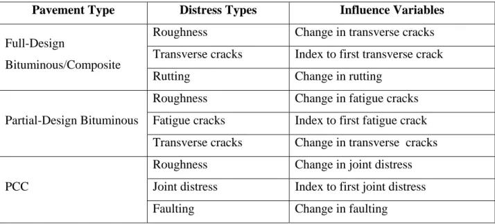
2.3.2.2 Determination of Distress Types, Influence Variables, and Distress States
Distress types define specific pavement deficiencies which trigger rehabilitation actions. Influence variables allow for prediction of future levels of distress types. The influence variable “index to the first distress, IFD” is used to differentiate between expected life cycles for
alternative rehabilitation treatments. The differences in future performance of different rehabilitation treatments can be handled properly through use of the index to the first distress. Table 2-2 shows distress types and influence variables.
2.3.2.3 Condition States (CS)
The condition state defines one particular combination of given levels of selected distress types and influence variables for a particular road category. In defining a condition state, the following sequence of variables is used: IFD, roughness, combination of primary distress type and rate of change for the first distress type, and combination of secondary distress type and rate of change for the secondary distress type. Total condition states will then be: 4x3x6x6=432 or 4x3x6x3=216. Since efficiency of the linear program and ease of developing performance
prediction models would increase with a reduced number of rates of change of distress, 216 condition states are normally used by KDOT.
Table 2-1 KDOT Road Categories (Kulkarni et al., 1983) Functional
Class Pavement Type
Roadway Width
(m) Traffic Loading Road Category
Interstate PCCP All 0-749 1 750-up 2 Composite 0-749 3 750-up 4 FDBIT* All 5 Other PCCP 0-87 6 88-162 7 163-up 8 Composite 0-87 9 88-162 10 163-up 11 FDBIT* <9.80 0-22 12 23-50 13 51-up 14 ≥9.80 0-22 15 23-50 16 51-up 17 PDBIT** <9.80 0-22 18 23-50 19 51-up 20 ≥9.80 0-22 21 23-50 22 51-up 23 * Full-Design Bituminous Pavement; ** Partial-Design Bituminous Pavement
Table 2-2 Distress Types and Influence Variables for Given Pavement Types
Pavement Type Distress Types Influence Variables
Full-Design
Bituminous/Composite
Roughness Change in transverse cracks Transverse cracks Index to first transverse crack
Rutting Change in rutting
Partial-Design Bituminous
Roughness Change in fatigue cracks Fatigue cracks Index to first fatigue crack Transverse cracks Change in transverse cracks
PCC
Roughness Change in joint distress Joint distress Index to first joint distress
Faulting Change in faulting
2.3.2.4 Feasible Maintenance and Rehabilitation Actions
After the list of actions or rehabilitation alternatives applicable to a given road category is prepared, feasible actions from this list for each condition state need to be specified. This would include actions that would adequately correct given distress levels. However, some actions may be permitted because of budget limitations, even if they do not correct the distresses. A list of maintenance and rehabilitation actions is shown in Table 2-3.
2.3.2.5 Costs of Different Actions
The total cost, C of action for pavements in condition state is given by the following: ) , (i k k i )) ( ), ( ), ( ( ) ( ), ( ), ( ( ) , (i k RMC R i D1 i D2 i CS R i D1 i D2 i C = k + k ) (i R ) ( 1 i D ) ( 2 i D ) ( ), ( ), ( (R i D1 i D2 i RMCk k a R(i),D1(i) D2(i) (2.1) where
= level of roughness corresponding to CS i;
= level of primary distress type corresponding to CS i; = level of secondary distress type corresponding to CS i;
= routine maintenance cost during the year following the action for a distress state specified by and ; and
)) ( ), ( ), ( (R i D1 i D2 i CSk ak ) ( ), (i D1 i R D2(i)
= construction cost of action on a pavement with the distress state specified by , and .
Table 2-3 List of Maintenance and Rehabilitation Actions (Kulkarni et al., 1983)
Feasible Action Pavement Type
FDBIT PDBIT Composite PCC
Do Nothing X X X X
Routine Maintenance X X X X
Seals X X X
Overlays X X X X
Surface Recycle with Overlay X X X
Cold Milling X X
Cold Mill with Hot Recycle X X X
Stress-Absorbing Membrane X X X
Type F Crack Repair X
Type P Crack Repair X
Cold Recyle with Overlay X
Joint Repair with PCC X X
Joint Repair with AC X X
PCC Pavement Patching X
PCC Concrete Overlay X
PCC Patching with Overlay X
Grinding PCC X
2.3.2.6 Optimal Rehabilitation Policies
An integrated set of computer programs, which accepts inputs and determines the optimal rehabilitation policies, is used in a NOS. The main steps are as follows:
1. An optimal steady state policy is determined for selected long-term performance standards for the given road category;
2. An optimal transition policy is determined in which optimal steady state distribution of road segments in different condition states is achieved; and
3. The optimal transition policy determined in Step (2) provides a recommended action for road segments in each condition state.
2.3.3 Project Optimization System (POS)
The objective of a POS is to determine the optimal assignment of one out of several feasible actions to each project scheduled for rehabilitation during the planning year. The
assignment should maximize total benefits over the portfolio of rehabilitation projects, subject to meeting constraints on the total available rehabilitation budget for the planning year and subject to matching the NOS performance requirements for each project. An integer program is used for this purpose.
The POS is specifically oriented toward engineering and technical needs of pavement management. The POS develops the potential for better performance for the total target cost of all the projects. This is accomplished by using site-specific cost and engineering data, and
actions not available to the NOS because of its broad network prospective. Components of a POS include a set of prediction models to estimate the probabilities of reaching different distress levels as a function of age, traffic, overlay thickness, and environmental factors; and an integer programming algorithm which determines the optimal assignment of one out of several feasible actions to each project scheduled for rehabilitation during the planning year (Kulkarni et al., 1988).
2.3.4 Pavement Management Information System (PMIS)
PMIS is a user-friendly operation to sort, query, and process data. It provides necessary information for the NOS and POS models. Relational database management (RDBM) software running in an OS/2 operating environment is used. The system is designed for the computer platform, Intergraph Interserve 3005.
2.4
Remaining Service Life (RSL)
The remaining service life (RSL) is the anticipated number of years that a pavement is in acceptable condition to accumulate enough functional or structural distress under normal
conditions, given that no further maintenance is performed or distress points equal to an as-defined threshold value (Baladi, 1991). RSL is calculated from the condition of the asset during that year and the projected number of years until rehabilitation is required. Once RSL is