DESIGN AND REAL-WORLD APPLICATION OF NOVEL
MACHINE LEARNING TECHNIQUES FOR IMPROVING
FACE RECOGNITION ALGORITHMS
Daniel S´aez Trigueros
Submitted to the University of Hertfordshire in partial fulfilment of the requirements for the degree of Doctor of Philosophy
Abstract
Recent progress in machine learning has made possible the development of real-world face recognition applications that can match face images as good as or better than humans. However, several challenges remain unsolved. In this PhD thesis, some of these challenges are studied and novel machine learning techniques to improve the performance of real-world face recognition applications are proposed.
Current face recognition algorithms based on deep learning techniques are able to achieve out-standing accuracy when dealing with face images taken in unconstrained environments. However, training these algorithms is often costly due to the very large datasets and the high computational resources needed. On the other hand, traditional methods for face recognition are better suited when these requirements cannot be satisfied. This PhD thesis presents new techniques for both traditional and deep learning methods. In particular, a novel traditional face recognition method that combines texture and shape features together with subspace representation techniques is first presented. The proposed method is lightweight and can be trained quickly with small datasets. This method is used for matching face images scanned from identity documents against face images stored in the biometric chip of such documents. Next, two new techniques to increase the performance of face recognition methods based on convolutional neural networks are presented. Specifically, a novel training strategy that increases face recognition accuracy when dealing with face images presenting occlusions, and a new loss function that improves the performance of the triplet loss function are proposed. Finally, the problem of collecting large face datasets is considered, and a novel method based on generative adversarial networks to synthesize both face images of existing subjects in a dataset and face images of new subjects is proposed. The accuracy of existing face recognition algorithms can be increased by training with datasets augmented with the synthetic face images generated by the proposed method. In addition to the main contributions, this thesis provides a comprehensive literature review of face recognition methods and their evolution over the years.
A significant amount of the work presented in this PhD thesis is the outcome of a 3-year-long research project partially funded by Innovate UK as part of a Knowledge Transfer Partnership between University of Hertfordshire and IDscan Biometrics Ltd1 (parthership number: 009547).
I would like to thank my supervisors Dr Lily Meng and Dr Margaret Hartnett for their invaluable guidance and support. Contrasting their different points of view has greatly stimulated my thinking and improved the quality of my research. I would also like to thank Dr Heinz Hertlein, who supervised the first year of my PhD, for his helpful guidance during those first steps.
I feel very fortunate to have had the opportunity to do my research in collaboration with IDscan Biometrics. I would not be writing this today if they had not selected me to work on the KTP project that led to this PhD thesis. I would like to thank Innovate UK for the funding that made it possible, and the fantastic KTP team for their input and feedback on my work. I would especially like to thank my KTP Adviser Gerry O’Hagan for all of his good advice on my personal and professional development. I am also very grateful to all my colleagues at IDscan for making it such a fun and inspiring place to work. I would like to thank my colleagues in the research team for creating such a positive and unique atmosphere for innovation. A special mention to Moneer Alitto for all the interesting discussions and sharing of ideas.
I would also like to thank the good friends that I have made in London in these past four years for making me feel like at home. Finally, I would like to thank my family, especially my parents. No matter how far I go, I can always count on their love, support and encouragement.
Contents
Abstract ii Acknowledgments iii 1 Introduction 1 1.1 Overview . . . 1 1.2 Outline . . . 3 1.3 Contributions . . . 4 2 Background 5 2.1 Feature Engineering . . . 5 2.1.1 Shape Features . . . 6 2.1.2 Texture Features . . . 8 2.1.3 Other Features . . . 9 2.1.4 Features in Practice . . . 9 2.2 Machine Learning . . . 10 2.2.1 Supervised Learning . . . 10 2.2.2 Unsupervised Learning . . . 13 2.2.3 Optimisation . . . 15 2.2.4 Hyperparameters . . . 16 2.2.5 Model Capacity . . . 172.2.6 Machine Learning for Computer Vision . . . 18
2.3 Deep Learning . . . 18
2.3.1 Feedforward Neural Networks . . . 18
2.3.2 Convolutional Neural Networks . . . 20
2.3.3 Deep Generative Models . . . 22
3.1.2 Evaluation Metrics . . . 27 3.2 Literature Review . . . 29 3.2.1 Geometry-based Methods . . . 30 3.2.2 Holistic Methods . . . 31 3.2.3 Feature-based Methods . . . 34 3.2.4 Hybrid Methods . . . 37
3.2.5 Deep Learning Methods . . . 39
3.3 Conclusions . . . 45
4 Shape and Texture Combined Face Recognition for Detection of Forged ID Doc-uments 47 4.1 Introduction . . . 48
4.2 Subject Review . . . 49
4.2.1 Face Alignment with Constrained Local Neural Field . . . 49
4.2.2 Scale-Invariant Feature Transform . . . 50
4.2.3 PCA and LDA for Face Recognition . . . 51
4.3 Proposed Method . . . 51
4.3.1 Face Normalisation . . . 51
4.3.2 Face Representation . . . 51
4.4 Experiments . . . 55
4.4.1 Evaluation Protocols and Datasets . . . 55
4.4.2 Training . . . 56
4.4.3 Results . . . 57
4.5 Conclusions . . . 58
5 Enhancing Convolutional Neural Networks for Face Recognition with Occlusion Maps and Batch Triplet Loss 60 5.1 Introduction . . . 61
5.2 Related Work . . . 62
5.3 Proposed Methods . . . 63
5.3.1 Occlusions Maps . . . 64
5.3.2 Batch Triplet Loss . . . 66
5.4 Experiments . . . 69
5.4.1 Performance on Occluded Faces . . . 70
5.5 Conclusions . . . 74
6 Generating Photo-Realistic Training Data to Improve Face Recognition Accu-racy 76 6.1 Introduction . . . 76
6.2 Related Work . . . 78
6.3 Proposed Method . . . 81
6.3.1 Conditional PGGAN . . . 81
6.3.2 Identity Latent Space . . . 82
6.3.3 Mutual Information Loss . . . 82
6.3.4 Proposed GAN . . . 83
6.4 Experiments . . . 84
6.4.1 Qualitative Analysis of Generated Images . . . 85
6.4.2 Augmenting Datasets with Synthetic Images . . . 86
6.5 Conclusions . . . 90
7 Conclusions 92
2.1 Specification of a simple CNN architecture. The input size of the network is a 32×
32×3 image and the output is a 10-dimensional vector. The number of filters in each convolutional layer is indicated implicitly as the output shape depth. Note that the activation function between layers has been omitted for brevity. . . 22 3.1 Public large-scale face datasets. . . 41 3.2 Decision boundaries for different variations of the softmax loss with margin. Note
that the decision boundaries are for class 1 in a binary classification case. . . 45 5.1 Mean classification accuracy and standard deviation of each occlusion mapO
gener-ated by different CNN models. . . 70 5.2 Mean classification accuracy and standard deviation of different CNN models
evalu-ated following the LFW unrestricted, labeled outside data protocol. . . 74 6.1 VGGFace subsets used for training the models. . . 85 6.2 Accuracy of discriminative models trained with depth-augmented datasets. The
re-ported accuracy corresponds to the TAR@FAR=0.01 obtained when evaluating the models on the IJB-A dataset. . . 87 6.3 Accuracy of discriminative models trained with width-augmented datasets. The
re-ported accuracy corresponds to the TAR@FAR=0.01 obtained when evaluating the models on the IJB-A dataset. . . 89
List of Figures
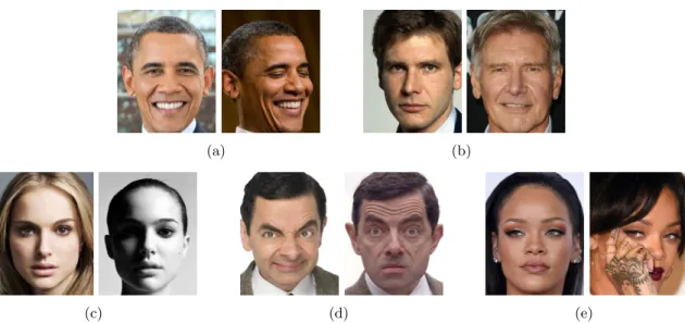
1.1 Typical variations found in faces in-the-wild. (a) Head pose. (b) Age. (c)
Illumina-tion. (d) Facial expression. (e) Occlusion. . . 2
2.1 Images filtered using the Sobel operator (a) Original image. (b) Horizontal gradient imageGx. (c) Vertical gradient imageGy. (d) Gradient imageGxy. . . 7
2.2 Facial landmark location using active shape model. . . 8
2.3 Computation of an LBP descriptor over a 3×3 window. . . 9
2.4 Feature matching using SIFT. . . 10
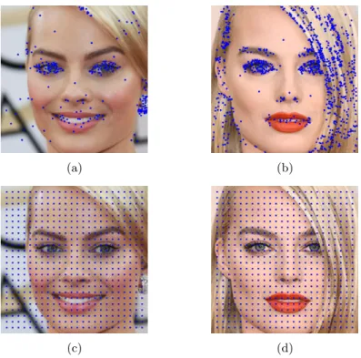
2.5 Keypoint vs dense feature extraction on aligned images. (a) and (b) SIFT keypoints. (c) and (d) Grid of equidistant points. . . 11
2.6 Linear classifier decision boundary. . . 13
2.7 Principal components of a 2D multivariate Gaussian distribution. The length of each arrow is proportional to the amount of variance in each direction. . . 14
2.8 Effect of the learning rate. Each red marker represents a gradient descent step. (a) Small learning rate. (b) Appropriate learning rate. (c). Large learning rate. . . 15
2.9 Lineal regression model using polynomials of different degrees to control the capacity of the model. The green circles represent points in the training set and the magenta triangles represent points in the test set. (a)Low capacity model. A polynomial of degree one underfits as it cannot fit the points in the training set. (b)Appropriate capacity model. A polynomial of degree three provides a good fit for the points in the training and test sets. (c)High capacity model. A polynomial of degree twelve overfits as it can fit the points in the training set but not the points in the test set. . 17
2.10 Fully-connected layer with two neurons connected to three inputs. . . 19
2.11 Convolutional layer with 6 filters. The blue region in the input volume represents the receptive field. Note how the depth of the filters has to match the depth of the input volume. Also note how the spatial dimensions of the output volume shrink since the convolution operation is not defined at the borders. . . 21
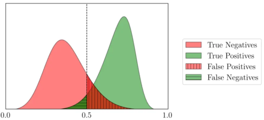
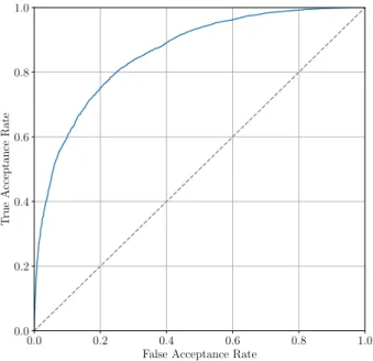
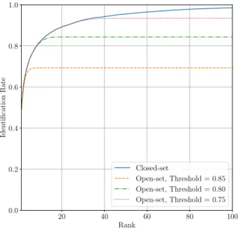
3.3 Distribution of similarity scores and a threshold of 0.5 in a verification system. Each possible outcome is indicated with a different combination of colour and pattern. . . 28 3.4 Example of a ROC curve generated using synthetic data. . . 29 3.5 Example of closed-set and open-set CMC curves generated using synthetic data. Note
that similarity scores below the thresholds are not taken into account for the compu-tation of the open-set CMC curves. . . 30 3.6 Top 5 eigenfaces computed using the ORL database of faces [70] sorted from most
variance (left) to least variance (right). . . 32 3.7 (a) Face image divided into 4×4 local regions. (b) Histograms of LBP descriptors
computed from each local region. . . 36 3.8 Typical hybrid face representation. . . 38 3.9 Original residual block proposed in [149]. W1 and W2 represent the weights of two
convolutional layers respectively and ReLU is a rectifier linear unit activation function. 43 3.10 Effect of introducing a margin min the decision boundary between two classes. (a)
Softmax loss. (b) Softmax loss with margin. . . 44 4.1 (a) Image printed on an ID document. (b) Image stored in the biometric chip of the
same ID document. . . 49 4.2 (a) Image gradients computed over a 16×16 pixel region. (b) Orientation histograms
computed over 4×4 pixel subregions using the gradients from (a). . . 50 4.3 Diagram illustrating the proposed face representation method. The numbers below
each block indicate the number of dimensions after each processing step. . . 52 4.4 Difference between features based on distances between pairs of landmarks and
fea-tures based on landmark locations. The Euclidean distance between the highlighted landmarks is 100.60 and 101.41 in (a) and (b) respectively, i.e. the relative distance between the landmarks remains almost the same in both face images. On the other hand, the misalignment of the landmark in the right corner of the mouth between (a) and (b) is 20.52. This indicates that using distances between landmarks provides extra robustness to facial expressions compared to using landmark locations. (a) Neutral facial expression. (b) Smiling facial expression. . . 53
4.5 ROC curves showing the effect that modifying the threshold(s) has on the recognition rates. (a) One threshold. (b) Two thresholds. Observe how the introduction of a lower thresholdtl allows to reduce the FRR at the expense of reducing the TRR and
having comparisons in which the result is undetermined. In real applications this is often desirable, as the number of negative comparisons is usually much lower than the number of positive comparisons. . . 55 4.6 ROC curves on the BiometricID dataset using the 4SF algorithm and the proposed
algorithm. . . 57 4.7 ROC curves on the Good, Bad and Ugly partition of GBU dataset using the 4SF
algorithm and the proposed algorithm. . . 57 5.1 (a), (d), (g) Mean image occluded at a random location with an occluder of 20×20,
20×40, and 40×40 respectively. (b), (e), (h) Occlusion mapsO20×20,O20×40, and
O40×40generated using model A and the corresponding occluders. The pixel intensity
of the occlusion maps represents the classification error rate when placing the occluder at each location. (c), (f), (i) Masked mean image using the occlusion mapsO20×20,
O20×40, andO40×40 respectively. . . 65
5.2 Example occluders used during training with different intensities, noise types and noise levels. (a) Salt-and-pepper noise. (b) Speckle noise. (c) Gaussian noise. . . 66 5.3 Example triplet from the CASIA-WebFace dataset. (a) Before triplet training. (b)
After triplet training. . . 67 5.4 (a) Distribution of positive and negative scores after training a CNN classification
model. (b) Distribution of positive and negative scores after fine-tuning the same CNN model with the standard triplet loss. Observe how even though the triplet training has been able to further separate the mean values of the two distributions, there is more overlapping between them, causing more false positives and/or false negatives . . . 68 5.5 Example images from the AR database. In each subfigure, the highlighted image on
the top left is the reference image (target image) used to compare against the other three images (query images). (a) Non-occluded. (b) Wearing sunglasses. (c) Wearing scarf. . . 71 5.6 AR database ROC curves (a) Non-occluded. (b) Wearing sunglasses. (c) Wearing scarf. 72 5.7 Example pairs from the LFW benchmark. (a) Positive pairs. (b) Negative pairs. . . 73 6.1 Proposed GAN model. . . 83 6.2 Generation of images of subjectsyin the training set with identity-related attributes
the method shown in Figure 6.2. The identity related attributes have been fixed for each row and the non-identity related attributes have been fixed for each column. Note that the highlighted images in the first column are real images from the training set. . . 86 6.5 Synthetic images of new subjects generated by the proposed GAN using the method
shown in Figure 6.3. The identity related attributes have been fixed for each row and the non-identity related attributes have been fixed for each column. . . 87 6.6 Comparison between synthetic images of new subjects and synthetic images of their
most similar subject in the training set. The top row of each of (a), (b), (c) contains synthetic images of a new subject and the bottom row of each of (a), (b), (c) contains synthetic images of their most similar subject in the training set. Note that the non-identity-related attributes only vary across the rows of (a), (b), (c) to restrict the comparison to the identity of the subjects. . . 88 6.7 Synthetic images generated by interpolating between two random vectors of identity
related attributesza
id,zidb and two random vectors of non-identity related attributes
za
Chapter 1
Introduction
1.1
Overview
Face recognition refers to the technology capable of identifying or verifying the identity of subjects in images or videos. The first face recognition algorithms were developed in the early seventies [1, 2]. Since then, their accuracy has improved to the point that nowadays face recognition is often preferred over other biometric modalities that have traditionally been considered more robust, such as fingerprint or iris recognition [3]. One of the differential factors that make face recognition more appealing than other biometric modalities is its non-intrusive nature. For example, fingerprint recog-nition requires users to place a finger in a sensor, iris recogrecog-nition requires users to get significantly close to a camera, and speaker recognition requires users to speak out loud. In contrast, modern face recognition systems only require users to be within the field of view of a camera (provided that they are within a reasonable distance from the camera). This makes face recognition the most user friendly biometric modality. It also means that the range of potential applications of face recognition is wider, as it can be deployed in environments where the users are not expected to cooperate with the system, such as in surveillance systems. Other common applications of face recognition include access control, fraud detection, identity verification and social media.
Face recognition is one of the most challenging biometric modalities when deployed in uncon-strained environments due to the high variability that face images present in the real world (these type of face images are commonly referred to as facesin-the-wild). Figure 1.1 shows some of these variations, including head poses, aging, occlusions, illumination conditions, and facial expressions. Examples of face recognition methods that are deployed in unconstrained environments are surveil-lance systems in which users are not aware that they are being recorded, or face verification systems that compare face images captured under any conditions. To simplify the problem, many face recog-nition algorithms constrain the distribution of face images (sometimes called theface space) to be analysed by one or several factors. For example, face recognition systems for border control typically
(a) (b)
(c) (d) (e)
Figure 1.1: Typical variations found in faces in-the-wild. (a) Head pose. (b) Age. (c) Illumination. (d) Facial expression. (e) Occlusion.
constrain the face recognition problem by making the user stand in a well-lit area and look at a high-resolution camera in a frontal pose. This normalisation of the image capturing process reduces the variability that face images present when analysed by a face recognition algorithm. Constraining the face space can be done in many other ways, e.g. by limiting the population size or reducing the maximum allowed age gap when comparing two faces. By taking into account these constraints, face recognition algorithms can be more specialised and achieve a higher accuracy. Note, however, that the distinction between constrained and unconstrained face recognition is not directly related to the applicability of face recognition in the real-world. A face recognition algorithm that works well in unconstrained conditions might not be the best choice when conditions are constrained. For this reason, the aim of this thesis is to propose novel machine learning techniques for improving the performance of face recognition applications that fall in both of these two categories.
Face recognition techniques have shifted significantly over the years. Traditional methods relied on hand-crafted features, such as edges and texture descriptors, combined with machine learning techniques, such as principal component analysis, linear discriminant analysis or support vector machines. The difficulty of engineering features that were robust to the different variations encoun-tered in unconstrained environments made researchers focus on specialised methods for each type of variation, e.g. age-invariant methods [4, 5], pose-invariant methods [6], illumination-invariant methods [7, 8], etc. Recently, traditional face recognition methods have been superseded by deep learning methods based on convolutional neural networks (CNNs). The main advantage of deep learning methods is that they can be trained with very large datasets to learn the best features to represent the data. The availability of faces in-the-wild on the web has allowed the collection of large-scale datasets of faces [9, 10, 11, 12, 13, 14, 15] containing real-world variations. CNN-based
CHAPTER 1. INTRODUCTION
face recognition methods trained with these datasets have achieved very high accuracy as they are able to learn features that are robust to the real-world variations present in the face images used during training. Moreover, the rise in popularity of deep learning methods for computer vision has accelerated face recognition research, as CNNs are being used to solve many other computer vision tasks, such as object detection and recognition, segmentation, optical character recognition, facial expression analysis, age estimation, etc.
Although significant progress has been made in recent years, a number of challenges remain. On one hand, methods based on CNNs have proven to be very effective for many applications. However, these type of methods require a large amount of training images to work well and can be very computationally expensive. As will be shown in Chapter 4, traditional methods are still relevant as they can achieve good accuracy in constrained settings. On the other hand, even when enough face images and computational resources are available to train CNN methods, the problem of recognising faces in-the-wild remains unsolved. This is because it is difficult to collect datasets that contain all the variations that will be seen in a real-world deployment. For this reason, reducing the data requirements of CNN methods is a fundamental problem. Chapters 5 and 6 of this thesis propose new techniques to tackle this issue, both by using better training schemes and by augmenting face datasets with synthetic data.
1.2
Outline
The body of this thesis is divided as follows:
• Chapter 2 provides the background needed for understanding traditional and deep learning approaches for computer vision applications.
• Chapter 3provides an introduction to face recognition and a comprehensive literature review of popular face recognition methods.
• Chapter 4 focuses on a particular constrained face recognition problem and proposes a new hybrid face recognition method to tackle it.
• Chapter 5proposes two new techniques to improve the performance of CNN-based methods for the recognition of faces in-the-wild.
• Chapter 6proposes a novel generative model to augment databases of faces with synthetic face images that can be used for training.
• Chapter 7 provides this thesis’ general conclusions by recapitulating the contributions and proposing further work for the future.
1.3
Contributions
This thesis’ contributions to the field are presented in Chapters 4 to 6. Although these chapters are not directly related, they follow a common theme of improving face recognition in real-world applications. They are written in a publication-style format as they are adaptations of academic papers (at the time of writing, a version of Chapter 4 [16] has been published in a conference proceedings; a version of Chapter 5 [17] has been published as a journal article; and a version of Chapter 6 is being prepared for submission). This section gives a short summary of each of these chapters and highlights the contributions made in this thesis.
Despite the recent success of deep learning methods, some face recognition applications are simple enough that can be solved with less computationally expensive methods that do not need to be trained with very large datasets. In Chapter 4 a traditional face recognition method to solve such a task is presented. In particular, the proposed method is used to match a face image scanned from an identity document presenting security features (e.g. watermarks and holograms) against a face image stored in the biometric chip of such a document. The proposed method uses a novel combination of texture and shape features together with subspace representation techniques. In addition, the adoption of two operating points to enhance the reliability of the final verification decision is proposed.
In Chapter 5 two contributions that improve the performance of CNNs for face recognition are presented. First, it is shown how facial occlusions remain a challenge when training a CNN using a dataset of faces collected from the web containing a low amount of face images presenting occlusions. Then, a technique to identify in which face regions occlusions can affect face recognition accuracy the most, and a data augmentation method that forces the CNN to learn discriminative features from all the face regions equally are proposed. The second contribution in this chapter is a modification of the popular triplet loss function often used when training CNNs for face recognition. More specifically, the proposed loss function can achieve a greater separability between the distributions of positive and negative scores by not only separating their means but also minimising their standard deviations.
Training data is arguably the most important component needed to achieve high accuracy using deep learning methods. However, collecting large-scale, good quality datasets is not always an easy task. In Chapter 6 this issue is addressed by proposing a novel generative adversarial network that can be used to synthesize both face images of existing subjects in a dataset and face images of new subjects. The experiments in this chapter show how models trained with different combinations of real data and synthetic data generated by the proposed generative model achieve better recognition accuracy than models trained with real data alone.
Chapter 2
Background
Computer vision is a field of computer science that aims to give computers the means to under-stand visual information in the same way as humans. All computer vision tasks require a high-level understanding of the numeric values that computers use to represent images. Some examples of clas-sic computer vision applications include object recognition, scene understanding, optical character recognition, image restoration and face recognition.
This chapter provides some technical background on the computer vision techniques that are most relevant to face recognition in general and to the understanding of this thesis in particular. The chapter is divided into three sections, starting from a basic approach of using hand-engineered features to extract information from images to more scalable and automatic approaches of using machine learning and deep learning for feature selection and feature learning.
2.1
Feature Engineering
In a computer system, images are represented by pixels arranged in a 2-dimensional grid. These pixels comprise numeric values that indicate colour intensity at each spatial location in an image. In the case of colour images, each pixel consists of multiple values, one for each colour channel (typically red, green and blue). One of the main challenges when dealing with images comes from the large number of possible combinations of pixel values that can yield an image. For example, the number of possible combinations of pixels in a 8-bit greyscale image with a low resolution of 32×32 pixels is 28×32×32. Even for such a low-resolution image, this number is extremely large and one of
the reasons why inferring meaningful information about the content of an image solely by looking at raw pixel values is not possible in general.
From a pattern recognition perspective, images are said to suffer from the curse of dimensionality as a result of their high-dimensionality. More specifically, when dealing with high-dimensional data such as images, the use of traditional statistical analysis methods to find patterns in the data becomes
unfeasible since the number of examples available to solve a problem is typically not enough to cover all the possible modes of variation. To overcome this problem, researchers have developed dimensionality reduction methods that extract relevant information from the data in the form of
features. At its core, feature engineering refers to the process of using domain-specific knowledge to develop features that transform high-dimensional data representations into discriminative lower-dimensional data representations.
2.1.1
Shape Features
One of the basic features used in computer vision is the presence of edges in an image. These edges correspond to sharp transitions in pixel intensity, or equivalently, to high-frequency contents in an image. The most common approach to computing edges is to perform high-pass filtering on an image by approximating the image gradient at each spatial location therein. Since the gradient is the directional derivative of the intensity in an image, locations that yield large gradients display large changes in pixel intensity, whereas locations that yield small gradients display constant pixel intensity.
An approximate image gradient is typically computed in the spatial domain by convolving an image with a small filter (also called kernel). For example, given an image I, the horizontal and vertical gradient imagesGx andGy can be computed using the well-known Sobel operator [18]:
Gx= +1 0 −1 +2 0 −2 +1 0 −1 ∗ I (2.1) Gy= +1 +2 +1 0 0 0 −1 −2 −1 ∗ I (2.2)
The spatial convolution operation (denoted by∗) involves sliding the filter across all spatial locations in an image and computing the dot product between the corresponding pixels and the values in the filter. The final gradient imageGxycan be computed as the gradient magnitude of both directional
components:
Gxy =
q
G2
x+G2y (2.3)
Figure 2.1 illustrates how the Sobel operator can be used to effectively detect edges in an image. Many early computer vision methods used edge detection as a mechanism for simplifying images. For example, Larry Robert’s Blocks World [19] proposed a way of inferring the 3D shape of objects by extracting and grouping their edges. Subsequently, some approaches were proposed to recognise more complex structures by combining basic object shapes [20, 21].
CHAPTER 2. BACKGROUND
(a) (b)
(c) (d)
Figure 2.1: Images filtered using the Sobel operator (a) Original image. (b) Horizontal gradient imageGx. (c) Vertical gradient imageGy. (d) Gradient imageGxy.
More advanced methods such as active contours models [22] and active shape models [23] are able to outline complex object shapes using edge information. In particular, active shape models use a deformable model of the assumed shape of an object, namely apoint distribution model, that is iteratively fitted to new examples. The basic approach is as follows:
1. Create a point distribution model (PDM) using a training set of examples with annotated landmarks.
2. Initialise the contour of a new object using the PDM.
3. Look for nearby edges in directions perpendicular to the current contour to generate a new contour that is closer to the edges of the object. The new contour is constrained by the PDM. 4. Repeat step 3 until convergence is achieved.
Active shape models and its variations are widely used to track the shape of deformable objects such as body parts. Figure 2.2 shows an application of active shape models for facial landmark location.
Figure 2.2: Facial landmark location using active shape model.
2.1.2
Texture Features
Although edges and shapes are very useful features for describing images, many computer vision tasks require more sophisticated solutions. For example, predicting whether two face images belong to the same subject based on the shape and locations of the facial landmarks alone would not provide very accurate results. This is because many faces have very similar shapes, as well as the fact that the face shape of a subject varies significantly due to different factors such as facial expression and head pose. In this case, it is also useful to have a representation of the texture of the face. This can be done by analysing the texture of the image at differentkeypointsusing texture descriptors.
For example, one popular texture descriptor is the local binary pattern (LBP) [24]. The basic method for computing LBP descriptors in an image is as follows:
1. Define a neighbourhood of fixed size around each pixel, for example, a 3×3 window.
2. Compare the centre pixel of each neighbourhood to each of its neighbours, giving a value of 0 if the centre pixel is greater than the neighbour and 1 otherwise. This gives a binary number (8 binary digits in the case of a 3×3 window) at each location which can be converted to a decimal number for convenience. This process is illustrated in Figure 2.3.
3. Create a histogram containing the frequency of each pattern (for a 3×3 window, the histogram has 28 bins). This histogram is the final feature vector and can be computed over the whole
image or over smaller regions.
LBP descriptors are fast to compute and provide a good estimation of the global texture of an image. Many variants of LBP have been proposed [25] and used to solve a wide range of applications such as face recognition [26], age classification [27] or palm print identification [28].
Considerable research has been done on feature extractors that are invariant to scale, orientation, illumination and other variations. These feature extractors typically comprise two stages, namely,
CHAPTER 2. BACKGROUND
feature localisation and feature description. During the feature localisation stage, a number of keypoints are automatically selected in the image. The goal is to select keypoints at locations in the image that remain detectable across different instances of the same object. At the same time, the keypoints need to be located in descriptive regions of the image (e.g. regions displaying constant pixel intensity should be avoided). In the feature description stage, a discriminative texture descriptor is computed around each selected keypoint. These descriptors can be used to match features between objects. Figure 2.4. shows an example of feature matching using thescale-invariant feature transform
(SIFT) [29], a popular feature extractor that follows this approach. Other similar methods include
speeded up robust features (SURF) [30] andbinary robust invariant scalable keypoints (BRISK) [31]. Another approach to feature extraction is dense feature extraction. In this case, instead of automatically selecting keypoints, the texture descriptors are computed on a grid of equidistant points. This is particularly useful when working with aligned images since the grid forces features to be extracted exactly at the same locations in every image. Figure 2.5 shows the difference between keypoint feature extraction and dense feature extraction on two aligned faces. Observe how, in this case, using dense features (Figures 2.5c and 2.5d) provides a much more accurate location for extracting consistent features across both images.
2.1.3
Other Features
Shape and texture features are the most commonly used features in computer vision as they can be computed on any image. More specialised features can be useful in certain situations. For example, features that use colour information can be useful for some problems such as skin colour detection [32], and motion features such as optical flow [33] are often used when dealing with videos. For a comprehensive and up-to-date survey of many of the features often used in computer vision, see [34].
2.1.4
Features in Practice
This section has shown how to obtain more descriptive and lower-dimensional representations of images by extracting different types of features. While features alone can be used to solve some simple problems, in general, they are not sufficient to solve more complex problems. For example, consider a face recognition system that relies on densely matching SIFT descriptors as shown in Figures 2.5c and 2.5d. Even if a grid of only 10×10 points is used, the resulting representation would still have a
Figure 2.4: Feature matching using SIFT.
very high-dimensionality (10×10×128, since each SIFT descriptor has 128 dimensions). Thus, it is still likely to suffer from the curse of dimensionality. This problem can be solved by dimensionality reduction techniques that use statistical analysis to find the most important dimensions, such as
principal component analysis(PCA). Moreover, a lot of problems cannot be solved by just extracting and matching features. These include classification problems which involve predicting the category to which an example belongs (e.g. optical character recognition), and regression problems which involve predicting a continuous value associated with a particular attribute of the data (e.g. age estimation).
Dimensionality reduction, classification and regression are typical examples of tasks that can be solved using machine learning techniques. In practice, most computer vision problems are solved by combining features with machine learning techniques. The next section describes basic machine learning concepts and some of the common algorithms used in computer vision applications.
2.2
Machine Learning
Machine learning is a field of artificial intelligence concerned with the development of algorithms that can learn from data. Machine learning algorithms can learn to perform tasks without being explicitly programmed to do so. This is useful in any situation where defining such tasks using a traditional computer programming paradigm would be overly difficult. Machine learning algorithms can be broadly classified as supervised and unsupervised learning techniques depending on how they use data to learn.
2.2.1
Supervised Learning
Supervised learning algorithms involve learning a functionf that maps inputsX to outputsY, i.e.
f :X →Y. To learn this mapping, a supervised learning algorithm must be trained with a set of
CHAPTER 2. BACKGROUND
(a) (b)
(c) (d)
Figure 2.5: Keypoint vs dense feature extraction on aligned images. (a) and (b) SIFT keypoints. (c) and (d) Grid of equidistant points.
output for that particular example. In computer vision, the inputs are typically pixels or features and the outputs are what needs to be predicted, e.g. coordinates of points in an image, probability that an object is present in an image, etc.
Since the goal is to develop algorithms that generalise to examples outside the training set, it is assumed that all the available examples for training and testing are independent and identically distributed (i.i.d.) samples from a common data generating distribution. The i.i.d. assumption implies that a functionf that provides a good fit on training data should also provide a good fit on test data. A discussion of what agood fit actually means is postponed to Section 2.2.5.
To find the function that best approximates the desired mapping, a loss or objective function needs to be defined. A loss function measures the error between a desired outputyand a predicted output ˆy=f(x). In general, most machine learning models learn functions that are controlled by a set of parametersθ. Therefore, the goal is to find the optimal parameters θ∗ from the set of all possible valuesΘthat minimise the loss over all the training examples:
θ∗= arg min θ∈Θ n X i L( ˆyi,yi;θ) (2.4)
of n 2-dimensional examples, each associated with a binary label, i.e {(x1, y1), ...,(xn, yn) | xi ∈
R2, yi ∈ {0,1}}. Since the model is linear, the algorithm needs to find a linear function of the inputs
w1x1+w2x2+b that separates the two classes, as illustrated in Figure 2.6. The output of a binary
linear classifier is as follows:
ˆ
y=σ(wTx+b) (2.5)
where
σ(z) = 1
1 +e−z (2.6)
is a sigmoid function that squashes the output of the linear mapping to a value between 0 and 1; and
w∈R2andb
∈Rare the parameters of the model. The output of the classifier ˆycan be interpreted
as the probability of the predicted class being 1, whereas its complement 1−yˆcan be interpreted as the probability of the predicted class being 0. Next, a loss function needs to be defined. In classification problems, it is common to use the cross-entropy loss, which for the binary case takes the form:
L(ˆy, y) =−ylog ˆy−(1−y) log(1−yˆ) (2.7) It can be shown that minimising the cross-entropy loss is equivalent to minimising the Kullback-Leibler divergence (which is a measure of distance between probability distributions) between the predicted probability distribution and the true probability distribution. The final step is to use an optimisation procedure to find the parameters θ = (w, b) that minimise the average loss over the training set (Equation 2.4). Once the classifier is trained, its parameters are fixed and Equation 2.5 is used to predict the class of new samples.
The binary linear classifier can be easily generalised to a multiclass linear classifier. In this case, each example is associated with a class label y that is a k-dimensional vector containing 0 at all indices except a 1 at the index of the correct class, wherekis the number of classes in the dataset. For example, for a classification problem with 5 classes, a sample belonging to the second class would have a label y= [0,1,0,0,0]. The output of the linear mapping in a multiclass linear classifier is a vector ofkclass scores that is normalised to a vector ofkclass probabilities that sum to one using the softmax function. Thus, the output of a multiclass linear classifier is:
ˆ y= softmax(WTx+b) (2.8) whereW ∈R2×k,b ∈Rk and softmax(z)i = ezi Pk jezj (2.9) For a multiclass classifier, the general form of the cross-entropy loss is used:
L( ˆy,y) =−
k
X
j
CHAPTER 2. BACKGROUND −4 −2 0 2 4 x1 −4 −2 0 2 4 x2
Figure 2.6: Linear classifier decision boundary.
More complex non-linear classifiers such as neural networks, discussed in Section 2.3, are very similar to the linear classifiers presented above but use non-linear functions to map inputs to a linearly separable space.
2.2.2
Unsupervised Learning
Unsupervised learning algorithms involve learning when the target outputs Y are not available. Unsupervised learning tasks typically require learning something about the data generating distri-bution. For example, clustering is an unsupervised learning task which consists of dividing a dataset into groups of examples with similar properties (e.g. grouping images that contain similar objects). A family of unsupervised learning algorithms relevant to this thesis are unsupervised generative models. In these models, the goal is to learn the data generating distribution itself. This can be useful for generating samples that are similar to those in the training set, by sampling from the estimated probability distribution learnt by the model. Generative models have gained a lot of attention recently in the deep learning community. Hence, their discussion is deferred to Section 2.3. As a practical example of an unsupervised learning algorithm, let us consider principal component analysis (PCA). PCA is a technique that uses an orthogonal linear transformation to project input data onto a space of uncorrelated dimensions. These dimensions are referred to as the principal components and they define the directions along which the variance in the data is the highest. An illustration of PCA is shown in Figure 2.7. PCA can be used for dimensionality reduction and data compression by selecting a subset of the principal components that account for the most variance as
−15 −10 −5 0 5 10 15 x1 −15 −10 −5 0 5 10 15 x2
Figure 2.7: Principal components of a 2D multivariate Gaussian distribution. The length of each arrow is proportional to the amount of variance in each direction.
the new basis vectors. The PCA dimensionality reduction algorithm can be summarised as follows: 1. Given a dataset of n d-dimensional examples {x1, ...,xn} in its matrix form X ∈ Rn×d,
normalise each feature to have zero mean and unit variance. This transformation ensures that the data is centred and that all the features have the same range of values.
2. Find the eigenvectors and eigenvalues of the covariance matrix cov(X) = 1
n
Pn
i xixTi. The
eigenvectors of the covariance matrix are the principal components and the eigenvalues indicate the amount of variance that each principal component accounts for.
3. Select thek < deigenvectors that correspond to theklargest eigenvalues. This can be done by fixing the output dimensionality tokprincipal components or by fixing the amount of variation to be retained and calculating how manyk principal components are needed.
4. Construct a matrixW ∈Rd×k of basis vectors from thek selected principal components.
5. Project the original datasetXonto the space spanned by thekprincipal components to obtain a lower-dimensional representationT =XW whereT ∈Rn×k.
The derivation of this algorithm is beyond the scope of this chapter and can be found in machine learning textbooks such as [35, 36].
CHAPTER 2. BACKGROUND x f ( x ) (a) x f ( x ) (b) x f ( x ) (c)
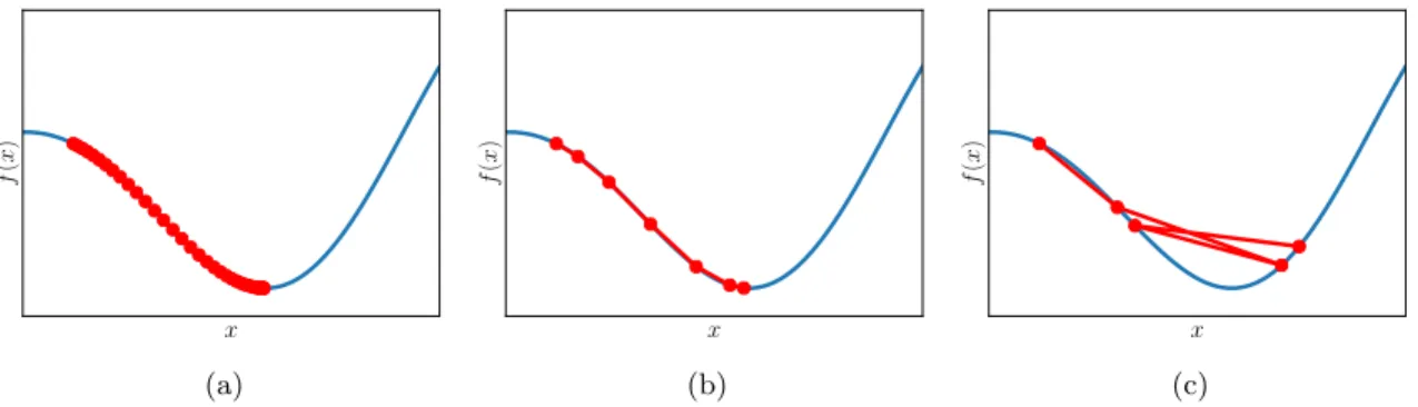
Figure 2.8: Effect of the learning rate . Each red marker represents a gradient descent step. (a) Small learning rate. (b) Appropriate learning rate. (c). Large learning rate.
2.2.3
Optimisation
Even though the solution of simple algorithms such as PCA can be obtained analytically, most machine learning algorithms require some form of optimisation to find their solutions. By optimi-sation it is meant a procedure that finds the optimal value of x that minimises (or maximises) a function f(x). This is usually denoted as x∗ = arg minf(x) (or arg max for maximisation). The most common form of optimisation used in machine learning is gradient-based optimisation.
Gradient-based optimisation can be described as follows: given a functionf(x), its first derivative
∂f(x)
∂x indicates how a small change in the inputxaffects the outputf(x). If the first derivative is
positive, a small increment to xwill result in a small increment to f(x). If the first derivative is negative, a small increment to x will result in a small decrement to f(x). Therefore, to find the value that minimisesf(x), small changes to xneed to be made with a sign that is opposite to the sign of the derivative. This optimisation procedure is known as gradient descent. More generally, when the input xis a vector, its gradient∇xf(x) is a vector containing all the partial derivatives
∂f(x)
∂xi . In this case, the value that minimisesf(x) can be found by making small changes to xin
the direction opposite to the gradient:
x←x−∇xf(x) (2.11)
where is a step size, commonly referred to aslearning rate, that scales the gradient update. If the learning rate is too small, the optimisation procedure might take a very long time to converge. On the other hand, if the learning rate is too large, the size of the increment toxmight overshoot the minimum of f(x) and the optimisation might not converge. The effect of the learning rate is illustrated in Figure 2.8.
Machine learning models are typically optimised by finding the parameters θ that minimise a loss functionLover all the training samples, as shown in Equation 2.4. The gradient of the loss can
be most accurately estimated by computing the average gradient over all the training samples: g(θ) = 1 n n X i ∇θL( ˆyi,yi;θ) (2.12)
In practice, the training sets used in machine learning can be very large, so it is common to estimate the gradient using a batch ofmnsamples. Since computing the gradient overmsamples is computationally cheaper than overnsamples, gradient descent can perform more frequent updates and hence converge faster. Note that if the batch size is too small, the gradient might be estimated poorly and the optimisation might take longer to converge. This version of gradient descent is known asstochastic gradient descent (SGD) [37]. The basic version of SGD is shown in Algorithm 1.
Algorithm 1Stochastic gradient descent.
Require: Learning rate
Require: Initial parametersθ
whilenot convergeddo
Sample a batch ofmsamples from the training set{(x1,y1), ...(xm,ym)}.
Estimate gradientg(θ)≈ 1 m Pm i ∇θL( ˆyi,yi;θ). Update parametersθ←θ−g(θ) end while
Most SGD implementations modify Algorithm 1 by decreasing the learning rate as the training progresses so that smaller steps are taken near the minimum of the loss function. Many variations of the update rule of the basic SGD algorithm exist. For example, the momentum update [38] can speed up the optimisation procedure and help it escape from shallow local minima by updating in the direction of an exponentially decaying average of past gradients. Other methods such as AdaGrad [39] and Adam [40] are able to automatically adapt the learning rate for each parameter
θi separately.
2.2.4
Hyperparameters
Most machine learning algorithms are controlled by a set of parameters that are not learnt by the model itself, e.g. the learning rate. These parameters are commonly referred to ashyperparameters. The usual way to select hyperparameters is to try different values and select the ones that provide the best results when the model is evaluated on a disjoint subset of the training set called the validation set. The final performance of the model is evaluated on a test set that should not be used to select the model’s parameters or hyperparameters. Therefore, the test set also needs to be disjoint from the training and validation sets.
CHAPTER 2. BACKGROUND x y (a) x y (b) x y (c)
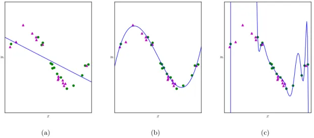
Figure 2.9: Lineal regression model using polynomials of different degrees to control the capacity of the model. The green circles represent points in the training set and the magenta triangles represent points in the test set. (a)Low capacity model. A polynomial of degree one underfits as it cannot fit the points in the training set. (b)Appropriate capacity model. A polynomial of degree three provides a good fit for the points in the training and test sets. (c) High capacity model. A polynomial of degree twelve overfits as it can fit the points in the training set but not the points in the test set.
2.2.5
Model Capacity
An important hyperparameter is the capacity of a model. The representational capacity of a model refers to the model’s ability to fit complex functions. For example, the linear classifier presented in Section 2.2.1 has low capacity as it can only represent first-order polynomials, as shown in Equa-tion 2.5. The capacity of that model can be increased by allowing the linear classifier to learn higher degree polynomials of the form b+Pk
i w T
i xi, where k varies the capacity of the model. Models
with low capacity can only learn simple functions and might result in the model performing poorly on the training data. This is known as underfitting. Models with high capacity can learn overly complicated functions that perform very well on the training data but poorly on the test data. This is known as overfitting. Figure 2.9 shows the effect of changing the representational capacity of a simple linear regression model. Notice how in the underfitting case the model is not able to fit the training data, whereas in the overfitting case the model fits the noise in the training data rather than the true data distribution.
Instead of controlling the capacity of a model by restricting the type of functions that the model can learn, a technique known asregularisation can be used to give the model a preference for some functions over others. For example, the L2 regularisation [41] method adds a term to the loss
function that controls the capacity of the model by giving a preference for learning small weights. Functions with small weights are smoother (i.e. they have less ups and downs) and therefore are
less prone to overfitting.
2.2.6
Machine Learning for Computer Vision
As explained in Section 2.1, feature engineering is an important step in most computer vision applications due to the high-dimensionality of images and videos. Even advanced machine learning algorithms such as support vector machines (SVM) [42] perform better when they are fed with low-dimensional features instead of raw pixel values.
For example, an image classification problem might be solved by densely extracting a large number of features from an image (e.g. LBP descriptors), performing dimensionality reduction (e.g. using PCA) and feeding the resulting lower-dimensional feature vector into a classifier (e.g. SVM). Even though such pipelines work well in many applications, their performance is often limited by the choice of features. Deep learning, discussed in the next section, eliminates the need to hand-engineer features, which are typically suboptimal, by automatically learning the optimal features for the task at hand.
2.3
Deep Learning
The term deep learning is commonly used to refer to deep artificial neural networks. An artificial neural network is a type of machine learning algorithm composed of interconnected nodes, called artificial neurons, arranged in layers. Simply put, each layer takes the outputs of the preceding layer as its inputs, applies a number of non-linear transformations to them, and sends its outputs to the next layer. The term deep is used when many layers are stacked together. The main motivation for using deep neural networks instead of other machine learning algorithms is that they are able to learn powerful features from raw data thanks to their hierarchical architecture and non-linear behaviour. This section provides a short summary of the main deep learning techniques used in this thesis. For a complete and up-to-date view of deep learning see [43].
2.3.1
Feedforward Neural Networks
The most basic type of neural network architecture is the feedforward neural network, also called
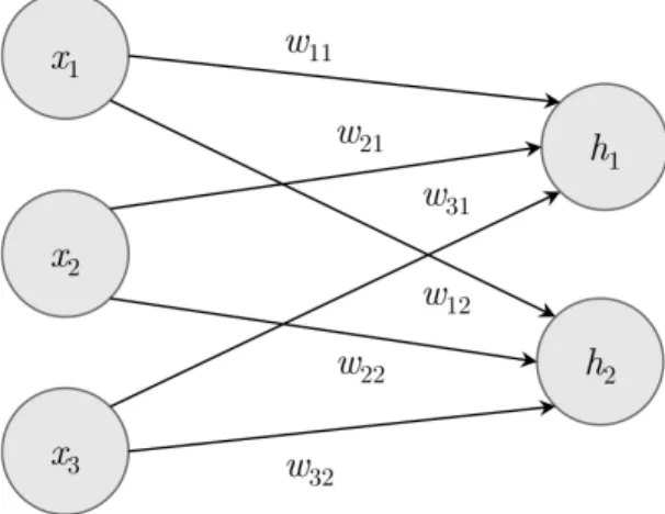
multilayer perceptron(MLP) [35]. In this network, the information only flows forward, i.e. there are no feedback connections which connect the outputs of previous time steps back into the network. The most basic component of an MLP is the fully-connected layer. In this type of layer, each neuron is connected to all of the layer’s inputs An example of a feedforward neural network with a fully-connected layer is shown in Figure 2.10. Each arrow in the figure represents a connection between the output of a neuronxi and an input of a neuronhj, and the strength of the connection
CHAPTER 2. BACKGROUND
Figure 2.10: Fully-connected layer with two neurons connected to three inputs.
is represented with a weightwij. The outputs h1 andh2 are calculated as follows:
h1=g(w11x1+w21x2+w31x3) (2.13)
h2=g(w12x1+w21x2+w31x3) (2.14)
wheregis a non-linear activation function such as the sigmoid function (Equation 2.6) or the rectified linear unit (ReLU) g(x) = max(0, x) [44]. In practice, it is common to add a bias termb to each non-linear transformation. More generally, a fully-connected layer withninputs andmoutputs can be written in its vectorised form as:
h=g(WTx+b) (2.15) where the matrix of weightsW ∈Rn×m and the vector of biasesb∈Rmare the parameters of the
layer. Note that a feedforward neural network with a single fully-connected layer is equivalent to a linear binary classifier if there is a single output and the activation function is a sigmoid function (Equation 2.5), or to a multiclass linear classifier if there are multiple outputs and the activation function is a softmax function (Equation 2.8).
The non-linear transformation described in Equation 2.15 can be chained to form feedforward neural networks with an arbitrary number of fully-connected layers. For example, the output of a feedforward neural network with three fully-connected layers is calculated as follows:
h1=g(W1Tx+b1) (2.16)
h2=g(W2Th1+b2) (2.17)
ˆ
where W1, W2, W3 and b1, b2, b3 are the weights and biases of the three layers respectively, x
is the input of the network, ˆyis the output of the network, and h1 andh2 are the outputs of the
intermediate layers, also called hidden layers. Note that if a linear function is used as the activation functiong, the entire neural network behaves like a linear model. By stacking layers with non-linear activation functions, neural networks are able to learn complex non-linear functions of their inputs commonly referred to as features (as they replace the traditional hand-engineered features used in other machine learning algorithms). Concretely, each layer in the network builds up on the features learnt by the preceding layer to learn features of increasing complexity. For example, in the case of images, the first layers might compute low-level features such as image gradients, whereas the last layers might compute high-level features such as the presence of particular objects in the image.
2.3.2
Convolutional Neural Networks
Aconvolutional neural network (CNN) [45, 46] is a type of feedforward neural network specifically designed to process data that can be spatially arranged such as images and videos. CNNs are mainly composed of convolutional layers. These layers differ from fully-connected layers in terms of how the neurons are connected to their inputs. In a fully-connected layer, each neuron is connected to all of the inputs, as shown above in Figure 2.10. In contrast, in a convolutional layer, each neuron is connected to a small region of neighbouring inputs called areceptive field. This type of connectivity pattern is known as local connectivity or sparse connectivity. The neurons in a convolutional layer work as filters that are convolved over the input image to producefeature maps. This transformation is analogous to the spatial convolution operation introduced in Section 2.1 but typically operates over three dimensions: width, height and depth. A feature mapH is calculated by computing the dot product between the weights in a filter and the corresponding elements in an input volume, plus a bias term. Thus, at each locationi,j,kin an input volumeX, the output of a convolutional layer is computed as follows:
Hi,j,k=
X
l,m,n
g(Xi+l,j+m,k+nWl,m,n+b) (2.19)
whereW is a filter,b is a bias term andg is an activation function. From this definition, it is easy to see that convolutional layers extract the same features from all the regions in an image, since the same filter W is used across all spatial locations i,j, k. This property is useful in many computer vision tasks. For example in object recognition, where the goal is to recognise an object that can appear anywhere in the image.
Since each filter computes one kind of feature, convolutional layers typically use many different filters in parallel to extract many kinds of features. Figure 2.11 shows how a 64×64×3 input volume convolved with 6 filters with a receptive field of 9×9 pixels produces a 56×56×6 output volume, i.e. 6 feature maps. Note that the width and height of the output volume can be preserved by zero-padding the input volume so that the filter can be applied at the borders.
CHAPTER 2. BACKGROUND
Figure 2.11: Convolutional layer with 6 filters. The blue region in the input volume represents the receptive field. Note how the depth of the filters has to match the depth of the input volume. Also note how the spatial dimensions of the output volume shrink since the convolution operation is not defined at the borders.
The number of parameters in a convolutional layer is drastically reduced compared to a fully-connected layer since the weights of a convolutional layer are shared across all spatial locations in the input (i.e. the same filter is slid over all spatial locations in the input). In a convolutional layer, the number of weights depends on the number of filters and the dimensions of their receptive fields rather than on the number of outputs. For example, to extract 50 different features from a 100×100×3 resolution image using a fully-connected layer, 150,000 weights are needed (50×100×100×3). On the other hand, to extract 50 different features from a 100×100×3 resolution image using a convolutional layer containing filters with a receptive field of 3×3 pixels, only 1,350 weights are needed (50×3×3×3). Note that the features extracted using a fully-connected layer are global (i.e. all the inputs are used in the computation), as opposed to the local features extracted using a convolutional layer. This means that extra layers are needed in a CNN to combine local features into global features. However, due to the reduced number of parameters, CNNs can stack many more layers (and therefore extract higher-level features) than fully-connected layers without risking overfitting.
Another important component of convolutional neural networks is subsampling [46]. The idea is to reduce the size of the feature maps as more layers are stacked. In this way, the number of parameters and the computational complexity of the model are reduced, and the final representation learnt by the model becomes more compact. The subsampling operation can be implemented with
poolinglayers or withstrided convolutions. Pooling layers are layers without parameters that simply calculate the average or the maximum value over small input regions. A strided convolution performs the same operation as a normal convolutional layer but skips some spatial locations. For example, a convolutional layer with a stride of 2 would skip half of the spatial locations and therefore produce a feature map with half the dimensions of the input.
Table 2.1: Specification of a simple CNN architecture. The input size of the network is a 32×32×3 image and the output is a 10-dimensional vector. The number of filters in each convolutional layer is indicated implicitly as the output shape depth. Note that the activation function between layers has been omitted for brevity.
Layer Filter size Stride Zero-padding Output shape Convolutional 5×5 1 Yes 32×32×32 Convolutional 3×3 1 No 30×30×32 Max pooling 2×2 2 No 15×15×32 Convolutional 3×3 1 Yes 15×15×64 Convolutional 3×3 1 No 13×13×64 Max pooling 2×2 2 No 6×6×64 Fully-connected - - - 512 Fully-connected - - - 10
to combine the outputs of all the feature maps and produce the final prediction output of the network. An example specification of a full CNN architecture is shown in Table 2.1.
2.3.3
Deep Generative Models
Generative models can learn an estimatepof the data generating distributionpdata in an
unsuper-vised fashion. Some models are able to learnpexplicitly and others can only learn to sample fromp. There are three type of deep generative models that have recently gained popularity: autoregressive models [47],variational autoencoders [48] and generative adversarial networks [49].
Autoregressive models [47] learn the probability distribution p explicitly by decomposing the probability of an input samplexas a product of conditional probabilities using the chain rule:
p(x) =Y
i
p(xi|x1, ..., xi−1) (2.20)
In a deep autoregressive model, the conditional probability of each element p(xi | x1, ..., xi−1) is
computed by a deep neural network. The main disadvantage of this approach is that during inference the samples are generated sequentially, as each element xi depends on the previously computed
elementsx1, ..., xi−1. This sequential generation becomes very slow when a deep neural network is
used to generate samples with a significant number of elements such as images [50] or sound waves [51].
Variational autoencoders [48] learn an approximation of the distributionpby maximising a lower bound L(x) ≤logp(x). In practice, this is done by maximising the probability of reconstructing the input samples using an encoder-decoder neural network and minimising the difference between the distribution learnt by the encoder and a simple prior distribution (e.g. a Gaussian distribution). Variational autoencoders are faster than autoregressive models as they can generate samples in a
CHAPTER 2. BACKGROUND
Figure 2.12: Vanilla generative adversarial network architecture.
single step. However, the samples generated by variational autoencoders tend to be blurry due to the mean squared error typically used in the reconstruction term.
Generative adversarial networks (GANs) [49] learn to generate samples without explicitly learning
p. A vanilla GAN consists of a generator networkGand a discriminator networkD. The generator networkGlearns to map samples zfrom a simple probability distributionpzto samplesG(z) that
look as if they were drawn from the data generating distributionpdata. The discriminator network
D is a binary classifier that outputs a scalar D(x) representing the probability that a sample xis real rather than generated (i.e. the probability thatxwas sampled frompdatarather than generated
by G). The term adversarial refers to the fact that the discriminator is trained to maximise the probability of assigning the correct label while the generator is trained to minimise the probability that the discriminator classifies generated samples correctly. Figure 2.12 shows the architecture of a vanilla GAN. The GAN training objective can be expressed as follows:
min
G maxD Ex∼pdata[logD(x)] +Ez∼pz[log(1−D(G(z)))] (2.21)
GANs are trained by optimising Gand D alternatively. Since the two networks have opposing optimisation objectives, the training converges when an equilibrium is reached. GANs can generate samples in a single step and, in general, produce better looking samples than variational autoen-coders. The main drawback of GANs is that their objective function is difficult to optimise in practice. Although, some alternatives such as the Wasserstein GAN [52] seem to alleviate this issue.
2.4
Conclusions
This chapter has given an overview of the most important techniques used to develop computer vision applications: feature engineering, machine learning and deep learning. The combination of hand-engineered features and traditional machine learning methods has been very successful for many years. However, in the last few years, deep learning techniques have quickly become the preferred approach for tackling complex computer vision tasks.
made in this thesis. In particular, feature engineering and traditional machine learning techniques are used in Chapter 4; convolutional networks are used in Chapter 5; and deep generative models are used in Chapter 6.
Chapter 3
Face Recognition
Starting in the seventies, face recognition has become one of the most researched topics in computer vision and biometrics. With the availability of large databases of face images and the appropriate computational resources, current algorithms based on deep neural networks are able to recognise faces in-the-wild with near human-level accuracy. One of the reasons why face recognition has attracted so much interest over the years is the wide range of commercial and law enforcement applications. Some of these include access control, surveillance, criminal identification, advertising and identity authentication. Another reason is the possibility of deploying face recognition systems without any user interaction. Other biometric modalities such as fingerprint or iris recognition are considered more robust than face recognition but are less appealing as they require the users to cooperate with the system.
This chapter starts with an overview of face recognition, its different modes of operation, and the most popular metrics used for evaluating them. After that, an extensive literature review of the subject is provided. The content of this chapter has been adapted for an academic review article1.
3.1
Overview
Face recognition refers to the capability of computers to correctly verify or identify face images. From a practical point of view, verification and identification are considered the two main face recognition modes of operation. Face verification refers to one-to-one matching and involves confirming the claimed identity of a subject2. Face identification refers to one-to-many matching and involves
finding the identity of a subject in a database of enrolled subjects. Face identification systems can be further divided into closed-set and open-set. In closed-set identification systems, it is assumed
1An online preprint is available asFace Recognition: From Traditional to Deep Learning Methods, arXiv preprint
arXiv:1811.00116, 2018.
Figure 3.1: Face recognition building blocks.
that all the queried subjects are already enrolled in the system, whereas in open-set identification systems any subject can be queried.
3.1.1
Building Blocks
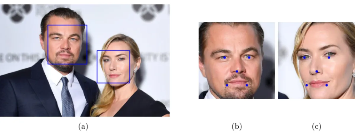
In practice, face verification and face identification systems are usually composed of the same building blocks. These are shown in Figure 3.1 and summarised below:
1. Face detection. A face detector finds the position of the faces in an image and (if any) returns the coordinates of a bounding box for each one of them. This is illustrated in Figure 3.2a. 2. Face alignment. The goal of face alignment is to scale and crop face images in the same way
using a set of reference points located at fixed locations in the image. This process typically requires finding a set of facial landmarks using a landmark detector and, in the case of a simple 2D alignment, finding the best affine transformation that fits the reference points. Figures 3.2b and 3.2c show two face images aligned using the same set of reference points. More complex 3D alignment algorithms (e.g. [53]) can also achieve face frontalisation, i.e. changing the pose of a face to frontal.
3. Face representation. At the face representation stage, the pixel values of a face image are transformed into a compact and discriminative feature vector, also known as a template. Ide-ally, all the faces of a same subject should map to similar feature vectors. Face representation is arguably the most important component of a face recognition system and the main subject of study in this thesis (it is also the focus of the literature review in Section 3.2).
4. Face matching. In the face matching building block, two templates are compared to produce a similarity score that indicates the likelihood that they belong to the same subject.
Note that the generic workflow depicted in Figure 3.1 can include extra building blocks for additional functionality. For example, some face recognition systems might use multiple images of a same subject to create a template. Similarly, face verification systems might apply a threshold to the similarity score to provide a definitivematch / not match decision. Furthermore, face identification systems typically need an extra building block to perform face matching between a query subject and all the subjects enrolled in the system. On the other hand, some face recognition systems